Publisher’s version / Version de l'éditeur:
Expert Systems with Applications, 39, 18, pp. 13193-13201, 2012-12-15
READ THESE TERMS AND CONDITIONS CAREFULLY BEFORE USING THIS WEBSITE.
https://nrc-publications.canada.ca/eng/copyright
Vous avez des questions? Nous pouvons vous aider. Pour communiquer directement avec un auteur, consultez la Questions? Contact the NRC Publications Archive team at
[email protected]. If you wish to email the authors directly, please see the first page of the publication for their contact information.
NRC Publications Archive
Archives des publications du CNRC
This publication could be one of several versions: author’s original, accepted manuscript or the publisher’s version. / La version de cette publication peut être l’une des suivantes : la version prépublication de l’auteur, la version acceptée du manuscrit ou la version de l’éditeur.
For the publisher’s version, please access the DOI link below./ Pour consulter la version de l’éditeur, utilisez le lien DOI ci-dessous.
https://doi.org/10.1016/j.eswa.2012.05.082
Access and use of this website and the material on it are subject to the Terms and Conditions set forth at
Data and knowledge visualization with virtual reality spaces, neural
networks and rough sets : application to cancer and geophysical
prospecting data
Valdés, Julio J.; Romero, Enrique; Barton, Alan J.
https://publications-cnrc.canada.ca/fra/droits
L’accès à ce site Web et l’utilisation de son contenu sont assujettis aux conditions présentées dans le site LISEZ CES CONDITIONS ATTENTIVEMENT AVANT D’UTILISER CE SITE WEB.
NRC Publications Record / Notice d'Archives des publications de CNRC:
https://nrc-publications.canada.ca/eng/view/object/?id=313fd8b5-e49a-4cd5-a515-48fabf6c9e84 https://publications-cnrc.canada.ca/fra/voir/objet/?id=313fd8b5-e49a-4cd5-a515-48fabf6c9e84
Data and Knowledge Visualization with Virtual Reality
Spaces, Neural Networks and Rough Sets: Application
to Cancer and Geophysical Prospecting Data
Julio J. Vald´esa
, Enrique Romerob
, Alan J. Bartona
a
Information and Communications Technologies National Research Council Canada
b
Departament de Llenguatges i Sistemes Inform`atics Universitat Polit`ecnica de Catalunya, Spain
Abstract
Visual data mining with virtual reality spaces is used for the representation of data and symbolic knowledge. High quality structure-preserving and max-imally discriminative visual representations can be obtained using a combina-tion of neural networks (SAMANN and NDA) and rough sets techniques, so that a proper subsequent analysis can be made. The approach is illustrated with two types of data: for gene expression cancer data, an improvement in classification performance with respect to the original spaces was obtained; for geophysical prospecting data for cave detection, a cavity was successfully predicted.
Keywords: Data and Knowledge Visualization, Visual Data Mining, Virtual Reality, Data Projection, Neural Networks, Rough Sets 1. Introduction
Knowledge discovery is the non-trivial process of identifying valid, novel, potentially useful, and ultimately understandable patterns in data [5]. In general, data under study are described in terms of collections of heteroge-neous properties, typically composed of properties represented by nominal, ordinal or real-valued (scalar) variables, as well as by others of a more com-plex nature, like images, time-series, etc. In addition, the information comes with different degrees of precision, uncertainty and information completeness (missing data is quite common). Patterns to discover are also of different kinds (geometrical, logical, behavioral, etc.).
Technological advancements in recent years are enabling the collection of large amounts data in many fields. For example, in the field of Bioinformat-ics, high-throughput microarray gene experiments are possible, leading to an information explosion. This increasing rates of data generation require the development of data mining procedures facilitating the in-depth understand-ing of the internal structure of data more rapidly and intuitively.
The complexity of many data analysis procedures makes it more difficult for the user to extract useful information out of the results from the tech-niques applied. Classical data mining and analysis methods are sometimes difficult to use, the output of many procedures may be large and time con-suming to analyze, and often their interpretation requires special expertise. Moreover, some methods are based on assumptions about the data which limit their application, specially for the purpose of exploration, comparison, hypothesis formation, etc., typical of the first stages of scientific investigation. The role of visualization techniques in the knowledge discovery process is well known. The human brain still outperforms the computer in understand-ing complex geometric patterns, thus makunderstand-ing the graphical representation of complex and abstract information directly appealing. A virtual reality (VR) technique for visual data mining on heterogeneous, imprecise and incomplete information systems was introduced in [24, 25]. Several reasons make VR a suitable paradigm for visual data mining: different representation models ac-cording to human perception preferences can be chosen, it allows immersion, it creates a living experience, it is broad and deep, and for using VR the user needs no mathematical knowledge and no special skills.
The purpose of this paper is twofold. First, to explore the construction of high quality VR spaces for visual data mining using a combination of neural networks and rough sets techniques. Second, to use the quality of the constructed VR spaces for classification tasks. The whole process is, in turn, divided into two steps. In the first one, both data and symbolic knowledge are transformed into VR spaces where their structure and properties can be visually inspected and quickly understood. In the second step, a proper subsequent analysis is made within the constructed VR spaces with the aim of obtaining good classification results. This latter analysis depends on the problem at hand. The approach is illustrated with two types of data: gene expression cancer data and geophysical prospecting data for cave detection. Three two-class gene expression cancer data sets were selected, represen-tative of three of the most important types of cancer in modern medicine: liver, stomach and lung. They are composed of samples from normal and
tumor tissues, described in terms of tens of thousands of variables, related to the gene expression intensities measured in microarray experiments. In the first step, neural networks for Sammon’s projection (SAMANN) [9, 13] are used for unsupervised structure-preserving mapping to low-dimensional feature spaces, where the corresponding VR spaces are constructed. Despite the very high dimensionality of the original patterns, high quality visual rep-resentations in the form of structure-preserving virtual spaces are obtained for every data set, which enables the differentiation of cancerous and non-cancerous tissues: the projected 3D spaces are polarized with two distribution modes, each one corresponding to a different class. In the second step, linear Support Vector Machines are constructed in the respective projected spaces, leading to an improvement in classification performance with respect to the original spaces.
A case of geophysical prospecting for underground caves is also studied. It is not the typical two-class presence/absence problem because only one class is known with certainty. In contrast, this is a problem with partially defined classes: the existence of a cave beneath a measurement station is either known for sure or unknown. In the first step, SAMANN and Non-linear Discriminant Analysis (NDA) networks [29, 12, 13] are constructed. SAMANN networks are used for unsupervised mapping to low-dimensional feature spaces, obtaining high quality structure-preserving visual represen-tations. NDA networks are used for supervised mapping to low-dimensional feature spaces where objects belonging to different classes are maximally dif-ferentiated. In the second step, the VR spaces and the NDA results allow to derive a fuzzy cave membership function and to predict unknown objects to the cave class. In one of the areas with higher values, a borehole drilled actually hit a cavity. Rough sets methods are applied for evaluating the information content of the original descriptor variables and for the extrac-tion of symbolic rules from the data. The general properties of the symbolic knowledge can be found with greater ease in the virtual reality space, and the structures of the knowledge base and the data were found very similar. 2. Virtual Reality Spaces for Visual Data Mining
Information systems were introduced in [16]. They have the form S = hU, Ai where U is a empty finite set called the universe and A is a non-empty finite set of attributes, such that each a ∈ A has a domain Va and an
evaluation function fa. The Va are not required to be finite. More generally,
heterogeneous and incomplete information systems should be considered [23]. A virtual reality (VR) space for the visual representation of informa-tion systems [24, 25], is defined as Υ = hO, G, B, ℜm, g
o, l, gr, b, ri. O is
a relational structure composed by objects and relations (O = hO, Γvi,
Γv = hγv
1, . . . , γvqi, q ∈ N +
and the o ∈ O are objects), G is a non-empty set of geometries representing the different objects and relations. B is a non-empty set of behaviors (i.e. ways in which the objects from the virtual world will express themselves: movement, response to stimulus, etc.). ℜm ⊂ Rm is
a metric space of dimension m (the actual VR geometric space). The other elements are mappings: go : O → G, l : O → ℜm, gr : Γv → G, b : O → B,
r is a collection of characteristic functions for selecting which of the orig-inal relations will be represented in the virtual world. The representation of an information system ˆS in a virtual world requires the specification of several sets and a collection of extra mappings: ˆSv = hO, Av, Γvi, O in Υ,
which can be done in many ways. A desideratum for ˆSv is to keep as many
properties from ˆS as possible. Thus, a requirement is that U and O are in one-to-one correspondence (with a mapping ξ : U → O). The structural link is given by a mapping f : ˆHn → ℜm. If u = hf
a1(u), . . . , fan(u)i and ξ(u) = o, then l(o) = f (ξ(hfa1(u), . . . , fan(u)i)) = hfav1(o), . . . , favm(o)i (fa
v i are the evaluation functions of Av).
Humans perceive most of the information through vision, in large quanti-ties and at very high input rates. The human brain is extremely well qualified for the fast understanding of complex visual patterns, and still outperforms computers. Several reasons make VR a suitable paradigm: i) it is flexible (it allows the choice of different representation models to better suit human perception preferences), ii) allows immersion (the user can navigate inside the data, and interact with the objects in the world), iii) creates a living ex-perience (the user is not merely a passive observer, but an actor in the world) and iv) VR is broad and deep (the user may see the VR world as a whole, and/or concentrate on specific details of the world). Of no less importance is the fact that in order to interact with a virtual world, only minimal skills are required [19].
3. Neural Networks for the Construction of Virtual Reality Spaces The typical desiderata for the visual representation of data and knowledge can be formulated in terms of minimizing information loss, maximizing
struc-ture preservation, maximizing class separability, or their combination, which leads to single or multi-objective optimization problems. In many cases, these concepts can be expressed deterministically using continuous functions with well defined partial derivatives. This is the realm of classical optimization where there is a plethora of methods with well known properties. In the case of heterogeneous information the situation is more complex and other techniques are required (see, for example [26, 27]).
In the unsupervised case, the function f mapping the original space to
the VR (geometric) space Rm can be constructed as to maximize some
metric/non-metric structure preservation criteria [11] as is typical in mul-tidimensional scaling [3], or minimize some error measure of information loss [18]. A typical error measure is:
Sammon Error = P 1 i<jδij X i<j (δij − ζij)2 δij (1) where δij is a dissimilarity measure between any two objects i, j in the
orig-inal space, and ζij is another dissimilarity measure defined on objects i, j
in the VR space (the images of i, j under f ). Usually, the mappings f ob-tained using approaches of this kind are implicit because the images of the objects in the new space are computed directly. However, a functional rep-resentation of f is highly desirable, specially in cases where more samples are expected a posteriori and need to be placed within the space. With an implicit representation, the space has to be computed every time that a new sample is added to the data set, whereas with an explicit representation the mapping can be used to compute directly the image of the new sample. As long as the incoming objects can be considered as belonging to the same population of samples used for constructing the mapping function, the space does not need to be recomputed. Neural networks are natural candidates for constructing explicit representations due to their universal function approx-imation property. If proper training methods are used, neural networks can learn structure-preserving mappings of high dimensional samples into lower dimensional spaces suitable for visualization (2D, 3D). Such an example is the SAMANN network. This is a feedforward network and its architecture consists of an input layer with as many neurons as descriptor attributes, an output layer with as many neurons as the dimension of the VR space and one or more hidden layers. The classical way of training the SAMANN network is described in [9, 13]. It consists of a gradient descent method where the
derivatives of the Sammon error are computed in a similar way to the classical backpropagation algorithm. Different from the backpropagation algorithm, the weights can only be updated after a pair of examples is presented to the network. As previously mentioned, the advantage of using SAMANN net-works is that, since the mapping f between the original and the VR space is explicit, a new sample can be easily transformed and visualized in the VR space. The same networks could be used as non-linear feature generators in a preprocessing step for other data mining procedures. A recent application of SAMANN networks for data visualization can be found at [4].
In the supervised case, a natural choice for representing the f mapping is a NDA neural network [29, 12, 13]. The NDA network is also feedforward with an input layer with as many neurons as descriptor attributes, an output layer with as many neurons as classes contain the decision attribute, a last hidden layer with a number of neurons equal to the dimension of the VR space and optionally other hidden layers. The NDA network is trained in a standard way [12, 13] to minimize the mean squared error.
4. Support Vector Machines for Classification
Support Vector Machines (SVMs) for classification can be described as follows [28]: the input vectors are mapped into a (usually high-dimensional) inner product space through some non-linear mapping φ, chosen a priori. In this space (the feature space), an optimal separating hyperplane is con-structed. By using a (positive definite) kernel function K(u, v) the mapping becomes implicit, since the inner product defining the hyperplane can be evaluated as hφ(u), φ(v)i = K(u, v) for every two vectors u, v ∈ RN. In the
SVM framework, an optimal hyperplane means a hyperplane with maximal normalized margin for the examples of every class (the normalized margin is the minimum distance to the hyperplane). When the data set is separable by a hyperplane (either in the input space or in the feature space), the maximal normalized margin hyperplane is called the hard margin hyperplane. When the data set is not separable by a hyperplane (neither in the input space nor in the feature space), some tolerance to noise is introduced in the model, associated to a parameter C that allows to control the trade-off between the margin and the errors in the data set. By setting C = ∞, the hard margin hyperplane is obtained.
To fix notation, consider the classification task given by a data set X = {(x1, y1), . . . , (xL, yL)}, where each instance xibelongs to the input space RN,
and yi∈ {−1, +1}. Using Lagrangian and Kuhn-Tucker theory, the maximal
margin hyperplane for a binary classification problem given by a data set is a linear combination of simple functions depending on the data:
fSV M(x) = b + L
X
i=1
yiαiK(xi, x) (2)
where the vector (αi)Li=1is the (1-norm soft margin) solution of the following
constrained convex optimization problem: Maximizeα PL i=1αi− 1 2 PL i,j=1yiαiyjαjK(xi, xj)
subject to PLi=1yiαi = 0 (bias constraint)
0 6 αi 6C i = 1...L.
(3)
The points xi with αi > 0 (active constraints) are named support vectors.
The most usual non-linear kernel functions K(u, v) are Gaussian, polynomial or wavelet kernels [15].
5. Symbolic Knowledge via Rough Sets and its Representation with Virtual Reality
The Rough Set Theory [16] bears on the assumption that in order to define a set, some knowledge about the elements of the data set is needed, in contrast to the classical approach where a set is uniquely defined by its elements. In the Rough Set Theory, some elements may be indiscernible from the point of view of the available information and knowledge is understood to be the ability of characterizing all classes of the classification [17].
A decision table is any information system of the form S = hU, Ai where A = A′∪ {d}, A′ are the condition attributes and d is the decision attribute.
The lower approximation of a concept consists of all objects, which surely be-long to the concept, whereas the upper approximation consists of all objects, which possibly belong to the concept. For any B ⊆ A an equivalence rela-tion IND(B) defined as IND(B) = {(x, x′) ∈ U2
|∀a ∈ B, fa(x) = fa(x
′ )}, is associated. A reduct is a minimal set of attributes B ⊆ A such that IND(B) = IND(A) (i.e. a minimal attribute subset that preserves the par-titioning of the universe). The set of all reducts of an information system S is denoted RED(A) (reduct computation is NP-hard, and several heuristics have been proposed [30, 21]). Reduction of knowledge consists of removing
superfluous partitions such that the set of elementary categories in the in-formation system is preserved, in particular, with respect to those categories induced by the decision attribute. Minimum reducts (those with a small number of attributes) are extremely important, as decision rules can be con-structed from them [2]. The algorithms for computing reducts and rules used in this paper are those of the Rosetta system [14].
6. Experiments with Gene Expression Cancer Data Sets
According to the World Health Organization, cancer is a leading cause of death worldwide (http://www.who.int/cancer/en). From a total of 58 million deaths in 2005, cancer accounts for 7.6 million (or 13%) of all deaths. The main types of cancer leading to overall cancer mortality are i) lung (1.3 million deaths/year), ii) stomach (almost 1 million deaths/year), iii) liver (662,000 deaths/year), iv) colon (655,000 deaths/year) and v) breast (502,000 deaths/year).
6.1. Data Sets Description
Three microarray gene expression cancer databases were selected, repre-sentative of three of the most important types of cancer in the world: liver, stomach and lung cancer. They share the typical features of these kind of data: a small number of samples (in the order of tens) described in terms of a very large number of attributes (in the order of tens of thousands), related to the gene expression intensities measured in microarray experiments. 6.1.1. Liver Cancer
The data were those used in [10], where zebrafish liver tumors were ana-lyzed and compared with human liver tumors. First, liver tumors in zebrafish were generated by treating them with carcinogens. Then, the expression pro-files of zebrafish liver tumors were compared with those of zebrafish normal liver tissues using a Wilcoxon rank-sum test. The original database had 20 samples (10 normal, 10 tumor) and 16, 512 attributes. As a result of this com-parison, a zebrafish liver tumor differentially expressed gene set consisting of 2, 315 gene features was obtained. This data set was used for comparison with human tumors. The results suggest that the molecular similarities between zebrafish and human liver tumors are greater than the molecular similari-ties between other types of tumors (stomach, lung and prostate). The data can be found at http://www.ncbi.nlm.nih.gov/projects/geo/gds/gds_ browse.cgi?gds=2220.
6.1.2. Stomach Cancer
The data were those used in [8], where a study of genes that are differ-entially expressed in cancerous and noncancerous human gastric tissues was performed. The original database contained 30 samples (22 tumor, 8 normal) that were analyzed by oligonucleotide microarray, obtaining the expression profiles for 6, 936 genes (7, 129 attributes). Using the 6, 272 genes that passed a prefilter procedure, cancerous and noncancerous tissues were successfully distinguished with a two-dimensional hierarchical clustering using Pearson’s correlation. However, the clustering results used most of the genes on the array. To identify the genes that were differentially expressed between can-cer and noncancan-cerous tissues, a Mann-Whitney’s U test was applied to the data. As a result of this analysis, 162 and 129 genes showed a higher expres-sion in cancerous and noncancerous tissues, respectively. In addition, several genes associated with lymph node metastasis and histological classification (intestinal, diffuse) were identified. The data can be found at http://www. ncbi.nlm.nih.gov/projects/geo/gds/gds_browse.cgi?gds=1210.
6.1.3. Lung Cancer
The data were those used in [20], where gene expressions of severely em-physematous lung tissue (from smokers at lung volume reduction surgery) and normal or mildly emphysematous lung tissue (from smokers undergo-ing resection of pulmonary nodules) were compared. The original database contained 30 samples (18 severe emphysema, 12 mild or no emphysema), with 22, 283 attributes. Genes with large detection P -values were filtered out, leading to a data set with 9, 336 genes, that were used for subsequent analysis. Nine classification algorithms were used to identify a group of genes whose expression in the lung distinguished severe emphysema from mild or no emphysema. First, model selection was performed for every al-gorithm by leave-one-out cross-validation, and the gene list corresponding to the best model was saved. The genes reported by at least four classifi-cation algorithms (102 genes) were chosen for further analysis. With these genes, a two-dimensional hierarchical clustering using Pearson’s correlation was performed that distinguished between severe emphysema and mild or no emphysema. Other genes were also identified that may be causally involved in the pathogenesis of the emphysema. The data can be found at http: //www.ncbi.nlm.nih.gov/projects/geo/gds/gds_browse.cgi?gds=737.
Parameters Liver
Neurons in the Hidden Layer {10,30}
Weights Ranges {(10,5),(10,10),(15,5)}
Learning Rates {(.1,.01),(.2,.01),(.2,.02)}
Momentum {0,.5,.7}
Number of Iterations {200,500,1000}
Random Seed Four different values
Presented Pairs at Every Iteration (All,50,100)
Parameters Stomach
Neurons in the Hidden Layer {10,30}
Weights Ranges {(10,5),(10,10),(15,5)}
Learning Rates {(.5,.1),(1,.1),(2,.1)}
Momentum {0,.5,.7}
Number of Iterations {200,500,1000}
Random Seed Four different values
Presented Pairs at Every Iteration (All,50,200)
Parameters Lung
Neurons in the Hidden Layer {10,20}
Weights Ranges {(50,5),(50,10),(60,5)}
Learning Rates {(.005,.0005),(.01,.001),(.02,.002)}
Momentum {0,.5,.7}
Number of Iterations {200,500,1000}
Random Seed Four different values
Presented Pairs at Every Iteration (All,50,200)
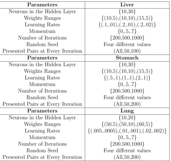
Table 1: Parameters used for the SAMANN networks with cancer data sets.
6.2. Experimental Settings
Data preprocessing. For stomach and lung data, each gene was scaled to mean zero and standard deviation one (original data were not normalized). For liver data, no transformation was performed (original data were already normalized).
Model training. For every data set, one-hidden layer SAMANN networks were constructed to map the original data to a 3D VR space. The Euclidean distance was the dissimilarity measure used in the original (δij) and the VR
(ζij) spaces. The activation functions were sinusoidal for the hidden layer
and hyperbolic tangent for the output layer. A collection of models was ob-tained by varying some of the network controlling parameters (table 1), for
a total of 1, 944 SAMANN networks for every data set.
6.3. Results
6.3.1. Visualization of SAMANN Results
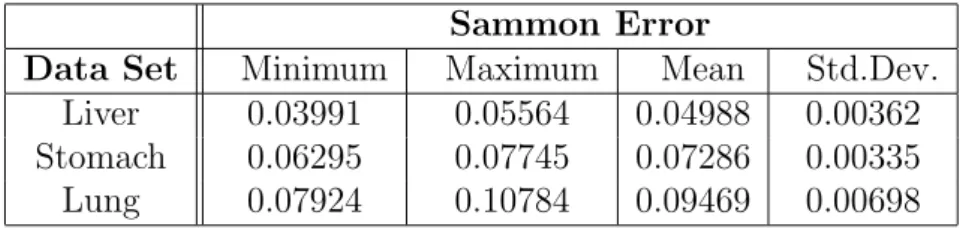
For every data set, we constructed the histograms of the Sammon er-ror for the obtained networks. The empirical distributions were positively skewed (with the mode on the lower error side), which is a good behavior. In addition, the general error ranges were small. In table 2 some statistics of the experiments are presented: minimum, maximum, mean and standard deviation for the best (i.e., with smallest Sammon error) 1, 000 networks.
Sammon Error
Data Set Minimum Maximum Mean Std.Dev.
Liver 0.03991 0.05564 0.04988 0.00362
Stomach 0.06295 0.07745 0.07286 0.00335
Lung 0.07924 0.10784 0.09469 0.00698
Table 2: Statistics of the best 1, 000 SAMANN networks obtained for cancer data sets.
Clearly, it is impossible to represent a VR space on printed media (nav-igation, interaction, and world changes are all lost). Therefore, very simple geometries were used for objects and only snapshots of the virtual worlds are presented. For simplicity, in all of the VR-spaces presented G ={dark spheres, light spheres}, B ={static} and the l function is based on the rep-resentation of f given by a SAMANN network. r is a single characteristic function for the relation C with the equivalent classes such that objects of one class will be represented as dark spheres and those of the other class by light ones.
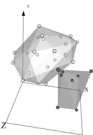
Figures 1, 2 and 3 show the VR spaces corresponding to the best obtained networks for the liver, stomach and lung cancer data sets respectively. Al-though the mapping was generated from an unsupervised perspective (i.e., without using the class labels), objects from different classes were represented in the VR space differently for comparison purposes. Transparent membranes wrap the corresponding classes, so that the degree of class overlapping can be easily seen. In addition, it allows to look for particular samples with ambiguous diagnostic decisions.
Figure 1: VR space of the liver cancer data set (Sammon error = 0.03991, best out of 1, 944 experiments). The space was generated from an unsupervised perspective, but classes are displayed for comparison purposes. Dark spheres: normal, Light spheres: cancerous samples.
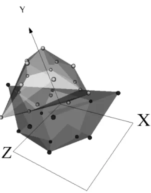
The low values of the Sammon error indicate that the spaces preserved most of the distance structure of the data, therefore giving a good idea about the distribution in the original spaces. The three VR spaces are clearly polarized with two distribution modes, each one corresponding to a different class. Note, however, that classes are more clearly differentiated for the liver and stomach data sets than for the lung data set, where a certain level of overlapping exists. The reason for this may be that mild and no emphysema were considered members of the same class (see section 6.1).
Since the distance between any two objects is an indication of their dis-similarity, the new point is more likely to belong to the same class of its nearest neighbors. In the same way, outliers can be readily identified, al-though they may result from the space deformation inevitably introduced by the dimensionality reduction.
6.3.2. Classification Results with SVMs
Since the projected spaces are polarized with two distribution modes, each one corresponding to a different class, a linear classification model is suitable from a supervised perspective. In our case, SVMs were used to that end, as explained next.
First, for every data set we obtained Sammon-projected data with dimen-sion values ranging from 3 to 20. For every dimendimen-sion, 2, 500 Newton mini-mization procedures were applied varying the initial point and the step size to obtain implicit representations of the original data. Similar to SAMANN
Figure 2: VR space of the stomach cancer data set (Sammon error = 0.06295, best out of 1, 944 experiments). The space was generated from an unsupervised perspective, but classes are displayed for comparison purposes. Dark spheres: normal, Light spheres: can-cerous samples.
networks, the Euclidean distance was the dissimilarity measure used in the original (δij) and the VR (ζij) spaces. The representations with smallest
Sammon error were selected. Then, for every dimension, a leave-one-out cross-validation was performed to the projected data with hard margin lin-ear SVMs (C = ∞).
Table 3 shows the best leave-one-out cross-validation performances ob-tained for every projected data set, together with the results obob-tained with the original dimensions. As it can be seen, classification performance im-proves in the projected spaces (with a very low dimension).
Figure 3: VR space of the lung cancer data set (Sammon error = 0.07924, best out of 1, 944 experiments). The space was generated from an unsupervised perspective, but classes are displayed for comparison purposes. Dark spheres: severe emphysema, Light spheres: mild or no emphysema. The boundary between the classes in the VR space seem to be a low curvature surface.
Data Set Dimension Test% Dimension Test%
Liver 16,512 90.0% 13 100.0%
Stomach 7,129 100.0% 4 100.0%
Lung 22,283 73.3% 11 90.0%
Table 3: Best leave-one-out cross-validation results for linear SVMs (C = ∞) with cancer data sets for original (left) and projected (right) data.
7. Experiments with Geophysical Prospecting Data
The proposed approach was applied to the detection of underground caves with geophysical data. Cave detection is a very important problem in civil and geological engineering. Sometimes the caves are opened to the surface, but typically they are buried and geophysical methods are required for de-tecting them. This task is usually very complex.
7.1. Data Set Description
The studied area contained an accessible cave (see figure 8 right). Geo-physical methods complemented with a topographic survey were used in the studied area with the purpose of finding their relation with subsurface phe-nomena [22].
The set of geophysical methods included 1) the spontaneous electric po-tential (SPdry) at the surface of the earth in the dry season, 2) the vertical
component of the electro-magnetic field in the VLF region of the spectrum, 3) the spontaneous electric potential in the rainy season (SPrain), 4) the
gamma ray intensity (Rad) and 5) the local topography (Alt). The raw data consist of these 5 fields (the attributes) on a spatial grid containing 1, 225 measurement stations (the data objects).
This is not the typical two-class presence/absence problem because only one class is known with certainty. In contrast, this is a problem with par-tially defined classes: the existence of a cave beneath a measurement station is either known for sure or unknown. Note, however, that this is not a one class problem, because two different classes exist. Since the classes are par-tially defined, a combination of unsupervised and supervised approaches is required.
7.2. Experimental Settings
Data preprocessing. In order to eliminate the data distortion introduced by the different units of measure and to reduce the influence of noise and regional geological structures, a data preprocessing process was performed consisting of: i) conversion of each physical field to standard scores. ii) model each physical field f as composed of a trend, a signal and additive noise: f (x, y) = t(x, y) + s(x, y) + n(x, y) where t is the trend, s is the sig-nal, and n is the noise component. iii) fit a least squares 2D linear trend ˆt(x, y) = c0+ c1x+ c2y and obtain the residual: ˆr(x, y) = f (x, y) − ˆt(x, y). iv)
convolve the residual with a low pass 2D filter to attenuate the noise com-ponent: ˆs(x, y) = PNk
1=−N
PN
k2=−Nh(k1, k2)ˆr(x − k1, y − k2), where ˆs(x, y) is the signal approximation, and h(k1, k2) is the low-pass zero-phase shift
digital filter. v) recompute the standard scores and add a class attribute indicating whether there is a known cave below the corresponding measure-ment station or if its presence is unknown. The pre-processed data will be called cave-prp-data.
Reducts from the original data set. The cave-prp-data set was dis-cretized using the boolean reasoning algorithm and the reducts were found
by Johnson’s algorithm [14]. A single reduct was found, consisting of all of the 5 original variables, proving that no proper subset of these variables exactly preserves the discernibility relation of the original data. That is, no lower dimensional space based on the power set of the original variables is discernibility-preserving. Thus, lower dimensional spaces based on non-linear combinations must be constructed for visualization.
Model training. A collection of experiments was conducted with one-hidden layer SAMANN networks in order to select adequate models for the visualization. Two-hidden layer NDA networks were used to construct a space where objects belonging to different classes are maximally differenti-ated. The activation functions were sinusoidal for the first hidden layer and hyperbolic tangent for the rest of layers. For the SAMANN networks, the Euclidean distance was the dissimilarity measure used in the original (δij)
and the VR (ζij) spaces. A collection of models was obtained by varying
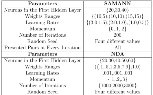
some of the network controlling parameters (table 4), for a total of 1, 260 for the NDA and 324 for the SAMANN networks respectively.
Parameters SAMANN
Neurons in the First Hidden Layer {20,30,40}
Weights Ranges {(10,5),(10,10),(15,15)}
Learning Rates {(3.0,1.5),(2.0,1.0),(1.0,0.5)}
Momentum {0,.1,.2}
Number of Iterations 200
Random Seed Four different values
Presented Pairs at Every Iteration All
Parameters NDA
Neurons in the First Hidden Layer {20,30,40,50,60}
Weights Ranges ({.1,.5,1,3,5,7,9},1.0)
Learning Rates .001,.001,.001
Momentum {.1,.2,.3}
Number of Iterations {1000,2000,3000}
Random Seed Four different values
Table 4: Parameters used for the SAMANN and NDA networks with the cave-prp-data set.
7.3. Results
7.3.1. Visualization of SAMANN Results
SAMANN networks mapped the original cave-prp-data 5-dimensional space to a 3D VR-space from an unsupervised perspective. The distribution of the Sammon error is shown in figure 4.
Figure 4: Left: Distribution of the SAMANN error (324 experiments) using SAMANN networks with the cave-prp-data set. Right: Distribution of the classification error of the cave class (1, 260 experiments) using NDA networks.
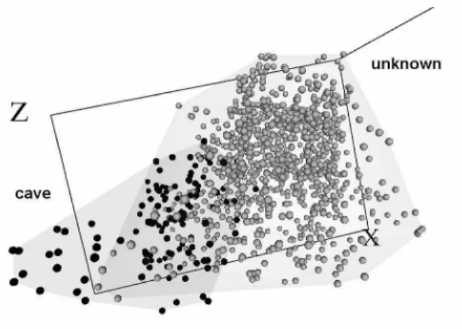
It is skewed towards the smaller errors end, which is a good behavior, with a mean of 0.0229 and a standard deviation of 0.0013 indicating that error values fluctuate within a narrow range. As an illustration, the VR-space corresponding to experiment 135 is shown in figure 5.
Figure 5: VR-space of the cave-prp-data set corresponding to experiment 135 (Sammon error = 0.0208). Objects of the cave class are dark. Objects of the unknown class are light (this is for comparison purposes only, since the mapping generating the space is unsupervised). Transparent membranes wrap the corresponding classes.
The low value of the Sammon error indicates that the space preserved most of the distance structure of the data, therefore, giving a good idea about the distribution in the original space. The space is clearly polarized with two distribution modes: one at the left hand side composed exclusively of cave objects, and another at the right hand side composed only of un-known objects. Since the distance between any two objects is an indication of their dissimilarity, objects of the unknown class closer to objects of the cave class are more likely to correspond to measurement stations having un-derground cavities than objects further away. In particular, those objects of the unknown class contained within the convex hull defined by the objects of the cave class are very interesting. It is also evident that only a smaller pro-portion of the objects of the unknown class are either contained, or close to the convex hull of the cave class, as expected from the typical lognormal-like distribution of many geological features.
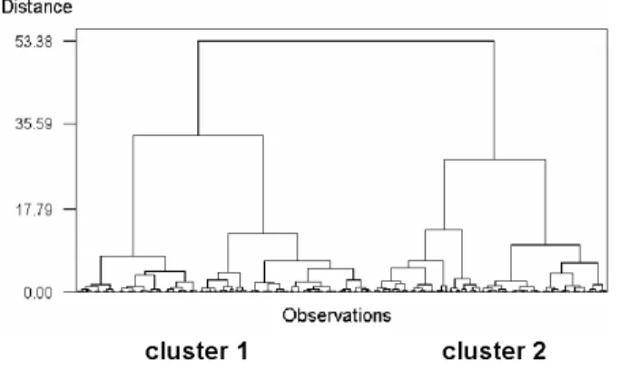
A hierarchical clustering using Euclidean distance and Ward’s method [1] (figure 6) clearly reveal the existence of two well defined clusters.
Figure 6: Dendrogram of the objects in the VR-space of figure 5 for the cave-prp-data set (Ward’s method using Euclidean distance).
Their nature is explained by the 2x2 contingency table defined by the membership with respect to the cave/unknown classes vs. those correspond-ing to the two clusters emergcorrespond-ing from the dendrogram. The table has a highly significant χ2
value (165.872), indicating the high degree of associa-tion between the existing classes (specially the cave class) and the formed clusters. Cluster 2 corresponds to the cave class containing 120 of the 121 cave objects and 419 unknown objects (likely candidates to belong to the cave class). Clearly, those in cluster 1 correspond to locations less likely to
have underground cavities beneath.
Cluster 1 Cluster 2 Total
Unknown 685 419 1,104
Cave 1 120 121
7.3.2. Visualization of NDA Results and Cave Membership Function
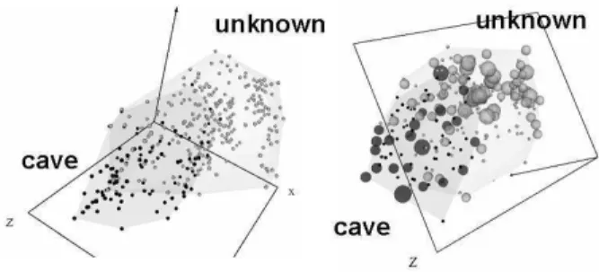
A structure preserving space is not necessarily class-discriminating and conversely. In a supervised situation, the information available from the decision attribute is used for constructing a space where objects belonging to different classes are maximally differentiated. NDA networks were used for that purpose. The distribution of the classification error for the cave class is shown in figure 4 (right) (the only determined class in the problem). The distribution exhibits a skewed-multimodal characteristic with the important modes shifted towards smaller error values (a good feature). Several networks have 0% classification error for the cave class and a representative of them is the one found in experiment 174.
A VR-space was built from a composition of the mapping function (ϕ) represented by that network, with a principal components transformation (P) given by f = (ϕ ◦ P) (figure 7).
Figure 7: VR-space maximizing class separability for the 1, 225 objects in the cave-prp-data set according to the (ϕ ◦ P) function. The classification error of the cave class is 0%.
The intrinsic dimensionality of this space is very close to one, and its shape indicates an almost linear continuum within and between the two classes. Conceptually, the objects at the two extremes represent the maximum expres-sion of a cavehood property, and its opposite, the maximum expresexpres-sion of be-ing solid rock, in geological terms. In between there is a gradation of the cave-hood property, which is actually a fuzzy concept. Let om ∈ O be the object
of the VR-space satisfying the property ((ϕ ◦ P)(om))pc1 ≤ ((ϕ ◦ P)(o))pc1 for all o ∈ O and let oM be the object such that d(om, oM) >= d(om, o)
for all o ∈ O, where d is the Euclidean distance and pc1 is the first
for caveness can be constructed as µc(o) = (1 − (d(om, o)/d(om, oM))). Note
that although a supervised approach was used, this formulation is based only on the information about the known class. The distribution of µ within the investigated area is shown in figure 8 (left).
Figure 8: Right: Map of the known cave. Left: Fuzzy membership function µc of the cave
class computed from the VR-space obtained from the NDA network (Extreme values: white=1, black=0). The white circle indicates the area where a borehole hit a cavity, not opened to the surface.
The behavior of µ depicts a very consistent and realistic geological pat-tern, where not only the known cave is correctly flagged with maximal mem-bership values, but also defines a collection of halos around the known cave with progressively decreasing values. In addition, other smaller areas with medium to high values are indicated, suggesting locations where other un-derground cavities could be expected. In particular, a borehole drilled at a location within the white circle of figure 8 (left) actually hit a cavity.
7.3.3. Visualization of Symbolic Knowledge
Symbolic knowledge in the form of production rules was extracted from the cave-prp-data set using rough set techniques, as explained in section 5. Structure preserving VR-spaces representing an information system with rules as objects can be constructed by minimizing the Sammon error (1). In this case the dissimilarity measure used for the original attributes was δij =
(1 − ˆsij)/ˆsij, where ˆsij is Gower’s similarity coefficient [6]. The Euclidean
were generated. Two representative examples are:
SPdry([−0.16981, ∗)) & V LF ([−0.75462, ∗)) &
SPrain([0.48744, ∗)) & Rad([−0.21015, ∗)) &
Alt([0.00346, ∗)) =⇒ unknown (123 objects)
SPdry([∗, −1.50209)) & V LF ([∗, −1.14882)) &
SPrain([∗, −0.46789)) & Rad([∗, −1.54413)) &
Alt([∗, −1.22398)) =⇒ cave (6 objects)
The approach described in [24, 25] for the construction of VR-spaces representing symbolic knowledge in the form of production rules was applied and the corresponding space is shown in figure 9 (left). When compared with figure 5 it is clear that the structures of the knowledge base and the data are very similar. An even clearer distribution is obtained if the rule base is pre-processed with the Leader clustering algorithm [7] in order to select representatives for subsets of similar rules and work with a smaller information system.
Such a space is shown in figure 9 (right) where the relative size of an object at a particular location in the VR-space is proportional to the number of similar rules within its neighborhood (therefore, of data concentration in the original feature space).
Figure 9: Left: VR-space with a representation of the 345 rules for the cave-prp-data set. Right: VR-space with the 231 most representative rules (sizes are proportional to the amount of similar rules at a given location). Dark objects: rules concluding about the cave class. Light objects: rules concluding about the unknown class.
This allows an easy identification of the most general rules from the more specific ones and also of knowledge granules. From the point of view of the
distribution of the most important objects, the space is strongly polarized, allowing the identification of the rules describing the properties of the physi-cal fields more accurately identifying the presence of underground caves and also the properties of the fields characterizing the areas most likely composed of solid rock. At the same time it allows the identification of the knowledge related with those objects of undetermined nature (i.e. from the undefined class).
8. Conclusions and Future Work
A combination of neural networks and rough set techniques was used for constructing virtual reality spaces for visual data mining suitable for representing data and symbolic knowledge. Good neural network models were found with the use of distributed computing techniques, that were used as mapping functions to produce high quality VR spaces where the properties of data and symbolic knowledge can be revealed.
For microarray gene expression cancer data sets, the obtained results show that a few non-linear features can effectively capture the similarity structure of the data and also provide a good differentiation between the cancer and normal classes. Linear Support Vector Machines constructed in projected spaces lead to an improvement in classification performance. However, in cases where the descriptor attributes are not directly related to class structure or where there are many noisy or irrelevant attributes the situation may not be as clear. In these cases, feature subset selection and other data mining procedures could be considered in a preprocessing stage.
Problems with partially defined classes can be approached successfully by combining unsupervised and supervised techniques. A method for con-structing membership functions in problems with partially defined classes is proposed which can be used as a forecasting tool, as illustrated with an example from geophysical prospecting. This approach can be extended to multiclass problems with partially defined classes.
Acknowledgments
This work was supported in part by the Ministerio de Ciencia e Inno-vaci´on (MICINN), under project TIN2009-13895-C02-01. This research was conducted in the framework of the STATEMENT OF WORK between the National Research Council Canada (Institute for Information Technology,
Integrated Reasoning Group) and the Soft Computing Group (Dept. de Llenguatges i Sistemes Inform`atics), Universitat Polit`ecnica de Catalunya, Spain.
References
[1] Anderberg, M., 1973. Cluster Analysis for Applications. Academic Press. [2] Bazan, J. G., Skowron, A., Synak, P., 1994. Dynamic Reducts as a Tool for Extracting Laws from Decision Tables. In: Symposium on Method-ologies for Intelligent Systems (Lecture Notes in Artificial Intelligence 869). pp. 346–355.
[3] Borg, I., Lingoes, J., 1987. Multidimensional Similarity Structure Anal-ysis. Springer-Verlag.
[4] Dzemyda, G., Marcinkeviˇcius, V., Medvedev, V., 2011. Large-scale Mul-tidimensional Data Visualization: A Web Service for Data Mining. In: European Conference on Towards a Service-Based Internet (Lecture Notes in Computer Science 6994). pp. 14–25.
[5] Fayyad, U., Piatesky-Shapiro, G., Smyth, P., 1996. From Data Mining to Knowledge Discovery: An Overview. In: et al., U. F. (Ed.), Advances in Knowledge Discovery and Data Mining. MIT Press, pp. 1–34.
[6] Gower, J. C., 1971. A General Coefficient of Similarity and Some of its Properties. Biometrics 27, 857–871.
[7] Hartigan, J., 1975. Clustering Algorithms. John Wiley & Sons.
[8] Hippo, Y., Taniguchi, H., Tsutsumi, S., Machida, N., Chong, J.-M., Fukayama, M., Kodama, T., Aburatani, H., 2002. Global Gene Expres-sion Analysis of Gastric Cancer by Oligonucleotide Microarrays. Cancer Research 62 (1), 233–240.
[9] Jain, A. K., Mao, J., 1992. Artificial Neural Networks for Nonlinear Projection of Multivariate Data. In: International Joint Conference on Neural Networks. Vol. 2. pp. 335–340.
[10] Lam, S. H., Wu, Y. L., Vega, V. B., Miller, L. D., Spitsbergen, J., Tong, Y., Zhan, H., Govindarajan, K. R., Lee, S., Mathavan, S., Murthy, K. R. K., Buhler, D. R., Liu, E. T., Gong, Z., 2006. Conservation of Gene Expression Signatures between Zebrafish and Human Tumors and Tumor Progression. Nature Biotechnology 24 (1), 73–75.
[11] Lee, J. A., Verleysen, M., 2007. Nonlinear Dimensionality Reduction. Springer.
[12] Mao, J., Jain, A. K., 1993. Discriminant analysis neural networks. In: 1993 IEEE International Conference on Neural Networks. pp. 300–305. [13] Mao, J., Jain, A. K., 1995. Artificial Neural Networks for Feature Ex-traction and Multivariate Data Projection. IEEE Transactions on Neural Networks 6, 296–317.
[14] Øhrn, A., Komorowski, J., 1997. Rosetta - A Rough Set Toolkit for the Analysis of Data. In: International Joint Conference on Information Sciences. Vol. 3. pp. 403–407.
[15] Ozer, S., Chen, C. H., Cirpan, H. A., 2011. A Set of New Chebyshev Kernel Functions for Support Vector Machine Pattern Classification. Pattern Recognition 44 (7), 14351447.
[16] Pawlak, Z., 1991. Rough Sets: Theoretical Aspects of Reasoning About Data. Kluwer Academic Publishers.
[17] Peters, G., Lingras, P., ´Sl¸ezak, D., Yao, Y., 2012. Rough Sets: Selected Methods and Applications in Management and Engineering. Springer. [18] Sammon, J. W., 1969. A Non-linear Mapping for Data Structure
Anal-ysis. IEEE Transactions on Computers C-18, 401–408.
[19] Simoff, S. J., Bhlen, M. H., Mazeika, A. (Eds.), 2008. Visual Data min-ing: Theory, Techniques and Tools for visual Analytics. Springer. [20] Spira, A., Beane, J., Pinto-Plata, V., Kadar, A., Liu, G., Shah, V., Celli,
B., Brody, J. S., 2004. Gene Expression Profiling of Human Lung Tissue from Smokers with Severe Emphysema. American Journal of Respiratory Cell and Molecular Biology 31, 601–610.
[21] Thangavel, K., Pethalakshmi, A., 2009. Dimensionality Reduction Based on Rough Set Theory: A Review. Applied Soft Computing 9 (1), 1–12.
[22] Vald´es, J., Gil, J. L., 1982. Application of Geophysical and Geomathe-matical Methods in the Study of the Insunza Karstic Area (La Salud, La Habana). In: First International Colloquium of Physical-Chemistry and Karst Hydrogeology in the Caribbean Region. pp. 376–384.
[23] Vald´es, J. J., 2002. Similarity-based Heterogeneous Neurons in the Con-text of General Observational Models. Neural Network World 12 (5), 499–507.
[24] Vald´es, J. J., 2002. Virtual Reality Representation of Relational Systems and Decision Rules: An exploratory Tool for Understanding Data Struc-ture. In: Theory and Application of Relational Structures as Knowledge Instruments / Meeting of the COST Action 274.
[25] Vald´es, J. J., 2003. Virtual Reality Representation of Information Sys-tems and Decision Rules: An Exploratory Tool for Understanding Data and Knowledge. In: International Conference on Rough Sets, Fuzzy Sets, Data Mining and Granular Computing (Lecture Notes in Artificial In-telligence 2639). pp. 615–618.
[26] Vald´es, J. J., 2004. Building Virtual Reality Spaces for Visual Data Mining with Hybrid Evolutionary-classical Optimization: Application to Microarray Gene Expression Data. In: IASTED International Joint Conference on Artificial Intelligence and Soft Computing. pp. 161–166. [27] Vald´es, J. J., Barton, A. J., 2005. Virtual Reality Visual Data Mining with Nonlinear Discriminant Neural Networks: Application to Leukemia and Alzheimer Gene Expression Data. In: International Joint Confer-ence on Neural Networks. pp. 2475–2480.
[28] Vapnik, V. N., 1995. The Nature of Statistical Learning Theory. Springer-Verlag, NY.
[29] Webb, A. R., Lowe, D., 1990. The Optimized Internal Representation of a Multilayer Classifier Performs Nonlinear Discriminant Analysis. Neu-ral Networks 3 (4), 367–375.
[30] Wr´oblewski, J., 2001. Ensembles of Classifiers Based on Approximate Reducts. Fundamenta Informaticae 47 (3-4), 351–360.