The analysis of river basins and channel networks using digital terrain data

THE ANALYSIS OF RIVER BASINS AND CHANNEL NETWORKS USING DIGITAL TERRAIN DATA

by

DAVID GAVIN TARBOTON

Bachelor of Science in Civil Engineering (Summa Cuin Laude) University of Natal, South Africa

(1981)

Master of Science in Civil Engineering Massachusetts Institute of Technology

(1987)

Submitted to the Department of Civil Engineering in partial fulfillment of the requirements

for the degree of Doctor of Science in Civil Engineering

at the

Massachusetts Institute of Technology September 1989

o Massachusetts Institute of Technology.

Signature of Author

Department of Civil Engineering September 1989

Certified by ,. ,,.,

Rafael L. Bras Thesis Supervisor

Accepted by

Acpeb ( -Ole S. Madsen

Chairran, Departmental Committee on Graduate Students

MASSACHUSETTS INSTIUTE OF TECHqn' fiGY

FEB

2

8 1990

THE ANALYSIS OF RIVER BASINS AND CHANNEL NETWORKS USING DIGITAL TERRAIN DATA

by

David Gavin Tarboton

Submitted to Department of Civil Engineering on September 7, 1989, in partial fulfillment of the requirements for the degree of Doctor of Science in

Civil Engineering ABSTRACT

This work examines patterns of regularity and scale in landform and channel networks. Digital elevation model data sets from throughout the United States are used as a data source.

First we consider the two-dimensional planform properties of channel networks. We find that networks as a whole may be regarded as space filling fractals, ie.., with fractal dimension 2. The scaling may be described by Horton's laws and provides a link between Horton length and bifurcation ratios.

Second we focus on elevation where the mean slope of rivers is characterized by a power law scaling with area. Investigations have recently used this to suggest that channel slopes are self-similar with magnitude or area as a scaling index. Our data indicates otherwise; in particular the variance of channel slope is larger than that predicted by simple self-similarity. The coefficient of variation of link slopes increases with area contributing to the link. This suggests multi-scaling. The scaling exponent for the standard deviation is approximately half the corresponding exponent in the relationship of the slope mean to magnitude or area. A model for channel slopes based on a point process of elevation drops along the channel is suggested. This model reproduces the observed multi-scaling properties when the density of elevation increments is related to area (or magnitude) as A- 0.

This scaling cannot hold in the limit of small area and must break at some point. We suggest that this break defines the lower bound scale for which channels exist and can therefore be used to determine the drainage density, the basic horizontal length scale associated with the dissection of the landscape by the channel network. This break in scale can also be detected as a break in the constant drop property, namely the empirical fact that the elevation drop along Strahler streams is on average constant. That the break in scale gives drainage density is justified using a stability analysis of landform development processes and empirical comparison of drainage densities from many DEM data sets. This work provides a rational way to extract channel networks with physically justifiable drainage density from digital elevation models.

Thesis Supervisor: Dr. Rafael L. Bras

Acknowledgements

I would like to thank my thesis supervisor, Professor Rafael L. Bras, for his guidance and support and from whom I have learned so much. Thanks also to the other members of my doctoral committee, Professors Ignacio Rodriguez-lturbe, Peter S. Eagleson and Michael A. Celia, who kept me motivated when I was skeptical and through their comments, criticisms and encouragement have contributed considerably to this work. In our research group, Garry Willgoose and Laurens van der Tak are thanked for their helpful comments and shared ideas. Thanks to MIT and the Parsons Lab, student and faculty, for the academic and intellectual environment where no limits are accepted and no idea is too wild to try.

Thanks to my wife Debbie for her love, understanding, support and sacrifice while here at MIT. Thanks to my parents Mike and Ann and siblings Ken and Judy who through my upbringing left me with the motivation and dedication necessary to complete this venture.

Elaine Healy and Carole Solomon efficiently typed this work from my appalling handwriting. Their patience is to be commended.

Support for this work was provided by the National Science Foundation (Grant No. ECE-8513556) and through a cooperative agreement between the University of Florence and MIT.

Table of Contents Page Abstract 2 Acknowledgement 3 Table of Contents 4 List of Figures 6 List of Tables 10 Chapter 1. Introduction 11 1.1 Scope 11 1.2 Outline 13

Chapter 2. Literature Review 15

2.1 Motivation 15

2.2 Terminology and Ordering Systems 16

2.3 Drainage Density, Dissection and Hillslope Scale 21

2.4 The Random Topology Model 23

2.5 Scaling in River Networks 26

2.6 Fractals and Scaling 35

2.7 Channel Network Evolution and Processes 44 Chapter 3. Data Analysis, Procedures and Techniques 54

3.1 Review 54

3.2 Data Sources and Accuracy 57

3.3 Procedures and Storage Conventions 59

3.4 Data 64

Chapter 4. Planar Space Filling Properties of River Networks 74

4.1 Introduction 74

4.3 Fractal Dimension and Horton 's Laws 81 4.4 Fractal Dimension and Tokunaga cyclicity 87

4.5 Planar Scaling Summary 91

Chapter 5. Slope Scaling 93

5.1 Introduction 93

5.2 Self-Similar Drop Model 94

5.3 Empirical Evidence of Scaling in Elevation 97

5.4 Link Slope Scaling Model 110

5.5 Conclusions 127

Chapter 6. Basic Scales in the Landform 128

6.1 Introduction 128

6.2 Slope-Area Scaling 129

6.3 The Constant Stream Drop Property 161

6.4 Localized DEM Procedures 188

6.5 Detailed Results 193 Chapter 7. Conclusions 203 7.1 Introduction 203 7.2 Planar Scaling 203 7.3 Slope Scaling 204 7.4 Basic Scale 204 7.5 Concluding Remarks 205 7.6 Future Research 206 References 210

Appendix: Computer Codes 221

List of Figures

Page Figure Title

2.1 Horton/Strahler ordering and link magnitude 18

2.2 Big Creek (CALD) Horton Analysis 19

2.3 Structurally Hortonian network with 27

bifurcation ratio 4

2.4 Sections of (A) a regular square-wave form and 37 (B) a randomized square-wave form

2.5 Graph of number of divider steps against 37

step length for the randomized square-wave form

2.6 Graph of measured length against scale of 37

measurement for the randomized square-wave form

2.7 Burwash TQ62 Richardson plots for 300' 41

and 400' contours

2.8 Variograms for the Aughwick, Pennsylvania (A) 42 and Shadow Mountain, Colorado (B) digital

elevation models

2.9 Characteristic form slope profiles 48

3.1 (a) Location map for 7.5 min Data sets 68

(b) Location map for 10 DMA Quadrangles 69

3.2 Channel networks from DEM with varying support 73 area compared to blue lines for the W15 data set

4.1 Ruler method results for typical river networks 76 4.2 Functional box counting results from W15 data set 77

4.3 Geometric stream length exceedance probability 79 4.4 Stream length (along stream) exceedance probability 80

5.1 St. Joe River and Big Creek location map 98

5.2 Link slopes for the St. Joe River, Idaho 100

5.3 Link slopes for Big Creek, Idaho 101

5.4 Link slope variances, St. Joe River, Idaho 102

5.5 Link slope variances, Big Creek, Idaho 103

5.6 St. Joe River link slopes normalized with n--0 104 5.7 Big Creek link slopes normali7ed with n-0.6 105

5.8 Model slope distributions by simulation 123

5.9 Normalized slope distributions from model by 124 simulation

5.10 Big Creek link slopes (not normalized) 125

6.1 CALD (Big Creek, Idaho) link slopes with support 130 area of 50 pixels used to extract network

6.2 Equilibrium slope profiles for superposed transport 134 functions

6.3 CALD (Big Creek, Idaho) residual sum of squares 138 from two phase regression as a function of switch

point

6.4 Slope versus area and two phase regression plot for

(a) W15 140 (b) W15A2S 141 (c) W7 142 (d) CALD 143 (e) SPOKBC 144 (f) NELK 145 (g) STJOE 146 (h) STJOEUP 147

(i) STREGIS 148

(j)

STREGISDMA

149

6.5 (a) Stream drops in W15 network extracted using 162 a support area of 50 pixels

6.5 (b) Stream drops in W15 network extracted using 163 a support area of 20 pixels

6.6 Stream drop distributions for the W15 network 165 6.7 Stream drops variation with order and support area for

(a) W15 167 (b) W15A2S 168 (c) W7 169 (d) CALD 170 (e) SPOKBC 171 (f) NELK 172 (g) STJOE 173 (h) STJOEUP 174

(i) STREGIS 175

(j)

STREGISDMA

176

6.8 Pixels identified by the Peuker and Douglas 190 Algorithm applied to the CALD data set

6.9 Pixels identified as one way local minima 191

in the CALD data set

6.10 Pixels that exceed accumulation area threshold 192 of 200 pixels in the CALD data set

6.11 Comparison of drainage density from different techniques 195 6.12 Schematic diagram of simulated slope profiles 199 6.13 Slope-area plots for simulated hillslopes profile A 200 6.14 Slope-area plots for simulated hillslope profile B 201

List of Tables

Page Table Title

2.1 Typical values of Exponents m and n in the empirical 47 relationships F c am Sn (Equation 2.44)

3.1 Binary Matrix Format 60

3.2 Network Storage Structure 61

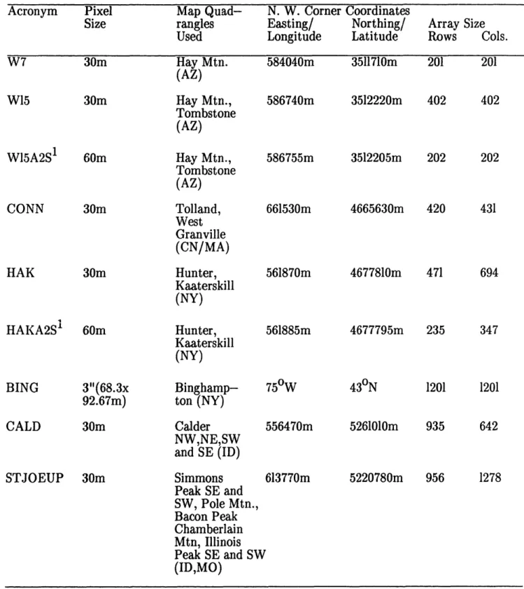
3.3 Digital Elevation Model Data Sets 65

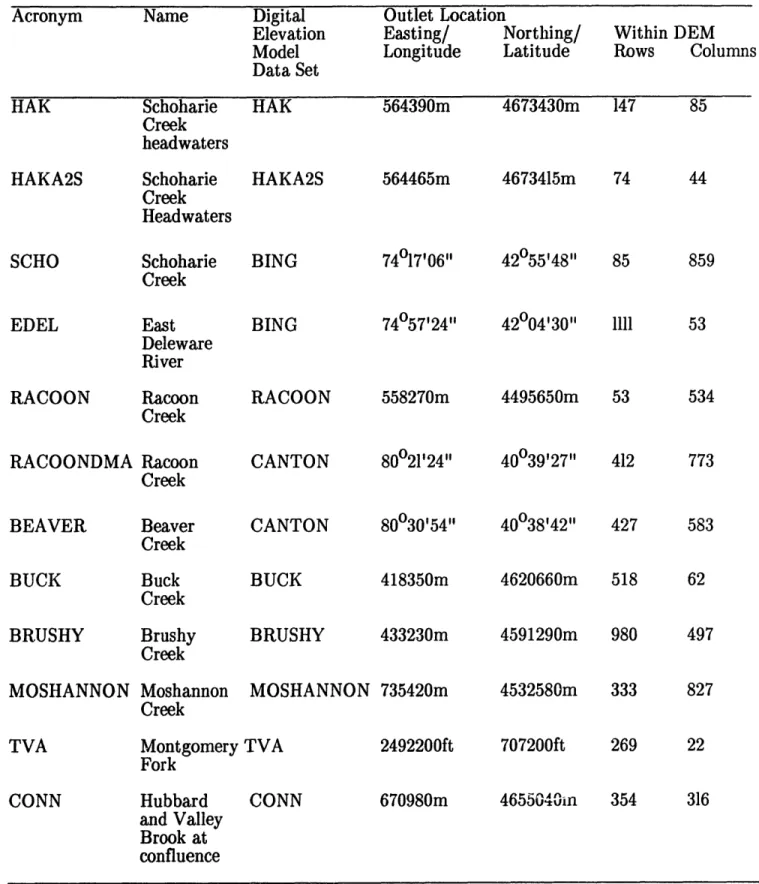
3.4 River Basins 70

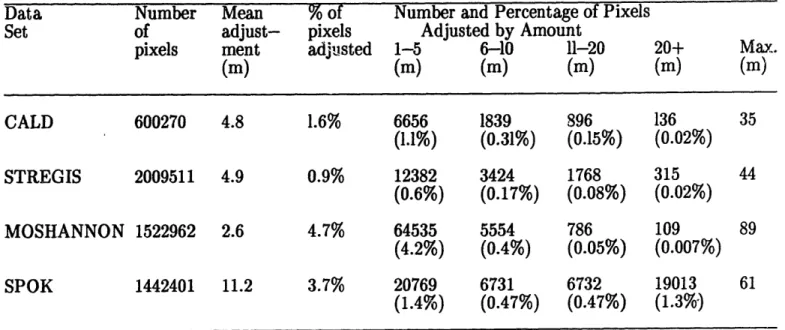
3.5 Statistics of Adjustments Required to Fill Pits 72 4.1 Network Geometry Data for Several River Networks 86

5.1 Big Creek Link Statistics 107

5.2 St. Joe River Link Statistics 108

5.3 Significance Tests for the Difference between 109 Normalized Slopes of Different Order

6.1 W15 Data set Link Lengths 139

Chapter 1 INTRODUCTION 1.1 Scope

Scientific and engineering work should always be based on the best available data that can be utilized effectively. This is also the case in hydrology where an important component of data is the channel network. The channel network defines the paths on the land surface along which water flows, and is a common component of flood routing or more general runoff routing models. Traditionally channel networks have been obtained from topographic maps. This requires that high resolution maps be available and for large basins is a tedious and time consuming task. Also channel networks on maps are scale-dependent and somewhat dependent on subjective judgment by the map maker. More recently the advent of computers has led to the development of digital elevation models (DEM b) as an alternative source of topographic information. These are gaining increasing use in the earth sciences, including hydrology, but especially in Geographic Information Systems. It is important that hydrologists keep abreast of the development of geographic information systems to ensure the availability of hydrologically relevant data and information. It is our opinion that DEM B are presently underutilized in hydrology. One objective of this work is to further develop the use of DEM ' for the analysis of channel networks and more generally hydrologic aspects of the whole landscape surface.

Another more scientific objective is research into the basic scales and scaling properties in river networks and the landscape. The composition, regularity, symmetries and scaling in natural river basins has interested scientists for a long time. Attempts to quantify and understand these have been motivated by the idea that landscapes are shaped and sculpted by rivers and the flow of water in them, so the shape of the landscape may hold information about runoff and river flow. We

attempt to answer the following questions. Are there fundamental length scales perhaps related to the processes or mechanisms involved in landform development? Are there landform properties that are scaling, i.e., invariant under transformations of scale, and if so over what range of scales does the scaling hold? The notions of drainage density (Horton, 1945), texture (Smith, 1950), and representative elementary area (Wood, et al., 1988) are measures of fundamental length scales. On the other hand, Horton's laws are really geometric scaling laws, implying that channel networks are self-similar over a range of channel orders or scales. Does this scaling have a physical lower limit at the drainage density, or is the lower limit just a matter of map resolution?

Through the use of digital elevation data we clarify and extend some of the older notions of scaling and symmetry of river networks, introducing modern concepts such as fractal dimension and multi-scaling. We also relate some of the scaling found to sediment transport and landscape forming processes, showing how the fundamental or basic scale associated with river networks, drainage density, can be interpreted as a scale where the dominating sediment transport process changes. Stable diffusive sediment transport processes dominate at the small scale leading to smooth hillslopes, while at large scale the instability caused by the convergence of surface flow and sediment transport results in channelization. This transition is detected in the data as a break in scaling. Below a certain scale the traditional scaling laws that characterize river networks no longer hold. The use of digital elevation data to detect this break in scaling lets us extract channel networks with a physically justifiable drainage density that is related to the basic scales present in the landscape and independent of subjective judgment by the map maker.

1.2 Outline

This work is divided into five main chapters, followed by a concluding chapter that summarizes the important results and an appendix giving details of the computer codes used.

Chapter 2 is a literature review and analysis of previous work. After reviewing the ideas that have motivated this study, we describe the terminology and ordering systems used. We then define drainage density, which is interpreted as the basic length scale associated with the dissection of the landscape by the river network. The random topology model is then described and scaling in river networks reviewed. The notion of fractal dimension used to characterize scaling is then presented, together with techniques to measure fractal dimension. We conclude the review with discussion of channel network and landscape evolution processes.

Chapter 3 goes into the technical details of the computer procedures used for processing DEM 's and extracting channel networks. It gives the data structures and conventions used. It also gives the sources of digital elevation data reviewing the procedures used in preparation of the data and discussing data accuracy. Tables at the end of Chapter 3 list the data sets used in this study.

Chapter 4 focuses on the planar properties of river networks. We show that in planform river networks can be regarded as space filling fractals and that this provides a relationship between the scaling of stream lengths and numbers given by

Horton's Laws.

Chapter 5 discusses the scaling of channel slope with area as a scaling index. Here DEM data shows that link slopes are not self-similar, but are characterized by a scaling that has coefficient of variation increasing with area. This scaling is such that the density of independent elevation increments has a negative power law scaling with area.

Chapter 6 focuses on the basic scale or drainage density. It first shows how the slope scaling of Chapter 5 breaks at a certain basic scale and then provides an interpretation of this in terms of sediment transport processes and a stability criterion. The fact that slope scaling is practically equivalent to a constant stream drop property then allows us to use the drop property as an alternative test for the break in scaling and measure of drainage density. A third measure of drainage density is obtained from localized DEM procedures and then the three measures of drainage density are compared for 21 DEM data sets.

Chapter 2

LITERATURE REVIEW 2.1 Motivation

There has been increasing interest during the last decade in the geomorphology of river networks and its relation to hydrology. The effort has been stimulated by the work of Rodriguez-lturbe and Valdes (1979) relating the instantaneous unit hydrograph to network morphology, and further work on this theme, Gupta et al. (1980), Rodriguez-Iturbe, et al. (1982), Troutman and Karlinger (1984; 1985). As a result investigators like Mesa (1986), Gupta and Mesa (1988), Abrahams (1984) have re-examined the structure of river networks and models describing that structure.

New sources of data, namely digital elevation models and powerful computers allow us to quickly test more alternatives and examine larger data sets than has ever been possible. O'Callaghan and Mark (1984) and Band (1986) have pioneered the extraction of channel networks from digital elevation models. The importance of scale issues and hydrologic similarity has received considerable interest recently [Conference proceedings, Gupta et al., (eds.), (1986); Rodriguez-Iturbe and Gupta (eds.) (1983)], with a realization that a basin scale approach is needed to understand the structure and similarity of river basins. It is hoped that this will ultimately lead to hydrologic predictions from ungauged basins.

The flow of water over long time scales has shaped river basins. Also the shape of river basins is a controlling factor in the generation of runoff and hydrologic response. This reciprocity is the fundamental reason for efforts to link hydrology and geomorphology and needs to be better understood. Through the analysis of a lot of digital terrain data, this work takes steps towards this understanding. The focus is on the scaling properties of river networks and landscapes, as well as the fundamental scales at which certain processes dominate or

where there may be changes from control by one process to another.

2.2 Terminology and Ordering Systems

The terminology used is basically that of Horton (1945), Shreve (1966), and in

common use in hydrogeomorphology.

A river network is idealized as a trivalent

planted tree, the root of which is the outlet or point furthest downstream. Sources

are points furthest upstream, and a point at which two upstream channels join to

form one downstream channel is called a junction or node. Exterior links are the

segments of channel between a source and the first junction downstream and

interior links are the segments of channel between two successive nodes or a node

and the outlet.

Each link has certain properties:

length along the stream;

geometric length, the distance between end points; height, the elevation difference

between upstream and downstream nodes; average slope, height divided by length;

contributing area, the total area draining through the link measured at the

downstream end and local area, the area draining directly into a link, i.e., not

through any other links.

Ordering systems are used to group or categorize links or segments of

channels. Ordering systems can work through the network from the root, or outlet,

upstream, or from each source, downstream or inwards. The upstream ordering

schemes have been unsuccessful so will not be discussed here.

A major contribution of Horton (1932, 1945) was the introduction of a

downstream ordering system. Strahler (1952, 1957) revised Horton b scheme to avoid

some ambiguities. The revised Horton/Strahler ordering system is as follows. All

exterior links have order 1. When 2 upstream links of the same order join the

downstream link has order increased by 1. When 2 upstream links of different order

join the downstream link takes the higher order of the two incoming upstream links.

Strahler streams are segments of channel consisting of links of the same order.

Another ordering system is the concept of link magnitude due to Shreve (1966). Here source streams or links have magnitude 1. At a bifurcation the downstream link takes magnitude the sum of the two incoming magnitudes. Thus the magnitude of each link represents the number of sources in the network draining into that link. Figure 2.1 shows the Horton/Strahler ordering system and concept of link magnitude.

Horton/Strahler ordering is usually used in characterizing a river network according to the Horton ratios.

Rb N 1 (2.1) R= L w (2.2) w-1

A

where Nw is the number of streams of order w, Lw is the mean length of streams of order w, Aw is the mean area contributing to streams of order w, and Sw is the mean slope of streams of order w. Rb, R1, Ra, and Rs are bifurcation, length, area, and slope ratios, respectively. Horton discovered that these ratios were approximately constant through semi-log plots of Nw , Lw, Aw, and Sw against order. The ratio or "Horton number" is obtained from the slope of the straight line fit to such plots, the procedure is called a "Horton analysis" (see Figure 2.2). Since the ratios are approximately constant, the above geometric descriptors are called

Legend

Order 2.

Order 3.

8 Link Magnitude

I I I i L -o~ -0 0 0 0 0 0 0 r) C*4 LU dOJC3 UJOOJIS I,; II n I -o C SUomBrIS Jo -ON I I0 [.if~ "o 'U3 L 0 rl0 _{0t 0"} Lu Io4ue L I, 0

I

i..,

(<

t

"Horton's laws." The area law above was not explicitly stated by Horton, and is due to Schumm (1956). Smart (1978, p. 131) notes that the Horton analysis has proved unsuccessful in the two major applications that Horton envisaged for it, namely the characterization of basins in different environments and the estimation of complete network properties by extrapolation of measurements from small-scale maps. Smart (1981) found this latter procedure to be highly inaccurate and badly biased. As far as characterizing basins in different environments the following are some of the studies that have found no significant differences in Horton ratios for different regions (Strahler 1952, 1957; Chorley, 1957; Woodruff, 1964; Eyles, 1968; Shreve, 1969). Abraharms (1972) found a significant correlation of Rb with relief. These deviations are more significant in terms of the link based analysis and random model to be discussed later.

Leopold and Miller (1956) extended Horton b ideas by showing that the log of many hydraulic variables are approximate linear functions of basin order. This behavior is due to the fact that most quantities depend strongly on the size of the drainage basin. A common measure of size or scale is basin area and the dependence of a general variable on area is often expressed, by a power law

X a Ab (2.5)

with b a constant. This implies

log X a log A (2.6)

and since order is proportional to log A (area law) the linear relationships with order follow.

Smart (1978) concludes that after 30 years of use the benefits from Horton analysis have been few and limited. Order just provides a simple objective (though not always consistent) measure of size or scale. It is not clear that order has any advantage for such purposes over other size related properties such as area and magnitude. Smart (1978) suggests, following Shreve (1966) that the link rather than Strahler stream segment should be regarded as the basic unit of network composition.

2.3 Drainage Density, Dissection and Hillslope Scale

The previous section presented the Horton/Strahler ordering system and concept of link magnitude as measures of size or scale of the network. These are topological, dimensionless, measures of size. They need to be related to the physical size, area, of the basin. This relationship will be through the drainage density which is a measure of the degree to which the basin is dissected by channels. It is also closely related to stream and link frequency (to be defined later), mean link length, and mean hillslope length. These are measures of a fundamental length scale associated with the dissection of the landscape by the river network. Horton (1932, 1945) defines the drainage density

L

Dd = (2.7)

where LT is the total length of streams and A is area. Horton suggested that the average length of overland flow or hillslope length could be approximated by 1/2 Dd. Smith (1950) measured the fundamental scale of topography in terms of a texture ratio, the number of contour crenulations divided by contour length. He essentially showed that texture was correlated with Dd so the notion of a well or poorly drained

basin corresponds to the notion of fine or coarse texture.

Horton defines stream frequency as

F=TN

(2.8)

where N is the number of Strahler streams. Link frequency F is similarly defined

using the number of links. Melton (1958) showed that Fs

was strongly correlated

with drainage density. Smart (1978) states that mean link length and link frequency

are also closely related to drainage density. If the mean area draining to a link is

t

_{(suggested by Shreve, 1967), where I is mean link length, the relationship is}

Dd = F =

(2.9)

We see that drainage density, stream or link frequency, mean link or

hillslope length and texture are all essentially measures of the same thing, the

fundamental horizontal length scale associated with how the channel network

dissects the landscape. The determination of this scale is generally dependent on

the resolution of the map used. Historically workers have called for the highest

resolution maps and/or field work to measure these quantities.

Mark (1983) discusses the differences between drainage networks obtained

from maps and field surveys, and the merits of various procedures such as use of

contour crenulations to "extend" the network. He concludes that first order basins

defined from contour crenulations on 1:24,000 maps do exist as topographic features

in the field.

However, the form has often been simplified by cartographic

generalization. Most first order basins defined on the map contain more than one

fluvial channel in the field.

Accordingly the exterior links drawn by contour

crenulations do not represent unbranched channels. The question arises in the

context of scaling and fractals (Mandelbrot, 1983) as to whether this notion of scale is well founded or whether the river networks dissect the landscape infinitely, requiring characterization as a scaling phenomena. This is one of the main questions addressed by this work and was recognized early by Davis (1899, p. 495), who wrote

"Although the river and hillside waste do not resemble each other at first sight, they are only the extreme members of a continuous series and when this generalization is appreciated one may fairly extend the 'river' all over its basin and up to its very divide. Ordinarily treated the river is like the veins of a leaf; broadly viewed it is the entire leaf."

2.4 The Random Topology Model

The notions of topologically distinct and topologically random channel networks due to Shreve (1966) have been fundamental to the assessment of network composition laws, such as Horton's laws. Topologically distinct networks as defined by Shreve (1966) are networks whose schematic map projections cannot be continuously deformed and rotated in the plane so as to become congruent. Shreve (1966) quantified the notion of "randomly merging channels" by proposing that all topologically distinct networks with a given number of links (i.e., fixed magnitude or scale) are equally likely. This is referred to as the first hypothesis of the random model. Using this idea Shreve (1966) showed that the most likely set of stream numbers were those that obeyed Horton's bifurcation law and furthermore that given a number of first order streams and basin order, the variability of number of streams of each order was topologically constrained to a narrow window around the straight line representing Horton's law. Shreve (1967) generalizes this result to infinite networks and shows that if mean link lengths, and areas draining to each link, are constant then Horton's length and area laws also follow. In infinite

networks Shreve (1967) obtains Rb = 4, RI = 2, Ra = 4. Smart (1968) first articulates the second hypothesis of the random model, namely that interior and exterior link lengths and the associated areas are independent random variables. The results of Shreve (1967) for Rb, Rt and Ra given above become expected values under this model. Shreve (1969) gives details of these results.

The fact that Horton ratios are approximately constant and that these constant values are reproduced by the random model is the main basis for Smart's (1978) conclusion above regarding the lack of utility of Horton analyses. The Horton ratios Rb, Rt and Ra may be seen as the effect of randomly merging channels and do not characterize different environments or networks. The same cannot be said about the slope ratio Rs since the random model says nothing about slope or elevation effects.

Shreve (1967) noted the connection between random networks and random walks. This connection is made concrete in terms of his representation of network topology symbolically as a string of Es and Is. The EI string is constructed as follows:

Start at the outlet and traverse the network always turning left at bifurcations and reversing direction at sources, until the outlet is again reached. During the traverse record an I, the first time a given interior link is traversed and an E the first time a given exterior link is traversed. Each link will be traversed twice but recorded only the first time.

A random network is equivalent to a random walk in which I's count +1 and E's count -1 and occur with equal probability. Gupta and Waymire (1983) point out that the equal probability of bifurcation and termination does not follow from the equal likelihood of topologically distinct random networks assumption and emphasize that the equal probability of termination and bifurcation should be added to the first random postulate. The IE string representation of network topology

coded as a binary string of O's and I's is also useful for computer storage of network topology information.

Random networks are also analogous to branching processes, which have been widely studied. Troutman and Karlinger (1984), Gupta et al. (1986), Mesa (1986), and Gupta and Mesa (1988) have used this fact to derive statistical properties of hydrologically important geomorphological functions, in particular the width function, tor topologically random networks. The width function L(x) is defined as the number of links, or points on the channel network at a distance x, measured along the channels, from the outlet, and was defined by Kirkby (1976). It is important because under the assumption of constant flow velocity in channels, it represents a time area diagram or unit response function for the channel network. The width function can be generalized by letting x be a more general measure of distance from the outlet. One such generalization is the link concentration function t(h) defined by Gupta, et al. (1986). Here the generalized distance is height or elevation above the outlet, denoted h.

The random model was very successful at "explaining" Horton's laws. However, using link based analyses Abrahams (1984) records many significant deviations from topologic randomness. In particular the random model predicts that cis and trans links occur with equal frequency. A cis link is where the upstream lower magnitude link and downstream lower magnitude link both enter on the same side of the link in consideration. A trans link is where they enter from opposite sides. James and Krumbein (1969) reported significantly more trans links than cis links and an abundance of short trans links in real basins.

These deviations may be a useful way of characterizing the difference between networks in different environments. Alternatively, they may be due to the geometric space filling constraints imposed when basins must be packed together on a surface (Goodchild, 1988) in which case they will be present in all networks,

irrelevant of the environment.

2.5 Scaling in River Networks

An important feature of the link based analysis and the topologically random network model is that the link provides a fundamental scale. Link length is a fundamental length scale related to drainage density by Equation (2.9). A basic length scale may not be desirable if it is dependent on the scale of map used, and is inconsistent with the notion of Davis (1899) of rivers extending over the whole land surface.

On the other hand, Horton's laws are scaling laws that relate properties at small scale (low stream order) to properties at large scale (high stream order). They characterize scaling at scales larger than the basic scale and may apply down to infinitesimally small scale if the notion of a lower bound basic scale is rejected. When analyzing scaling, the notion of self-similarity (defined formally in Section 2.6) is important. The use of Horton's laws as exact descriptors of scaling is not consistent with self-similarity. A network constructed to have Horton's bifurcation law hold exactly cannot be self-similar and have low order streams flow directly into streams more than one order higher. To see this consider the third order network shown in Figure 2.3 with bifurcation ratio 4. There must be 4 second order and 16 first order streams. To maintain self-similarity and the same bifurcation ratio, 4 first-order streams must flow into each second order stream. There are no first-order streams remaining to flow directly into the third-order stream. This property is not borne out in practice.

Furthermore it seems reasonable to assume at least as a first approximation that the area draining directly into each link is approximately constant. This constant is the average area draining first-order streams A1 (since they are single

SOrder 1.

SOrder

3.

links). Now the number of links in any network is 2n-1 so the total area draining a

basin order

w

is

A = AI(2n - 1)

(2.10)

Now Horton's bifurcation law [Equation (2.1)] implies

n = R

_(2.11)

n=Rb

so we get

A = AI(2R

- 1)

(2.12)

from which

I

_l

Thus for Rb constant, R

is dependent on order, i.e., not constant. The bifurcation

and area laws together with constant average area per link are mutually

inconsistent.

This inconsistency is also manifested if instead of assuming the area draining

directly into each link constant, we assume the area draining directly into each link

is proportional to link length (with mean link length constant, these amount to the

same thing). The average length of streams of order

w

is LIR

so the average area

draining directly into a stream of order

w

is AIR

. Hack (1957) sums these areas

to get

A

l]/[Re/Rb -1]

which implies

Ra = Rb{[(Re/Rb)" - l]/[R/Rb - l]} / w - (2.15)

Again for R, and Rb constant, Ra is not constant. Perhaps these are the reasons why Horton never stated an area law (leaving it to Schumm, 1956). Horton (1945) believed in the constancy of the length of overland flow (1/2 Dd) which amounts to area draining directly into a stream being proportional to length and leads to the inconsistency of the area law with other laws.

This discrepancy is not resolved by assuming differences between external and internal links. If we denote the average area draining internal links a, (with ai

< A1), we get analogously to Equation (2.15)

Aw = (A1 - ai )RW l + ai Rrl[(Rf/Rb)w l]/[Re/Rb 1]

(2.16)

which cannot be expressed as an exponential function of w, as would be required for an area law.

These inconsistencies are resolved in the cyclic scaling model suggested by Tokunga (1978). Horton/Strahler ordering is still used, with the interpretation of the lowest order streams being the smallest resolvable at the scale of resolution being used. Order is used as a relative, rather than absolute measure, with 0 the highest order stream and Q-l, Q-2, ..., lower order streams, extending to infinitely small order. The absolute order Q is never actually known, but the differences

between orders of different streams gives an idea of their relative sizes. Denote the

number of streams of order i flowing laterally into a higher order stream of order

j

by 1ji. Tokunaga (1978) suggests that j-jk (k

>

_{0) are on average independent of}

j,

denoted

k = jej-k

and that, furthermore

K k

K--ek-l

is on average constant. The two parameters

l and K are analogous to Rb in that

they completely describe the number of streams of each order. In practice K and f1

suffer from some of the same drawbacks as Rb. They show scatter within particular

networks, do not distinguish between qualitatively different networks from different

environments and cluster around approximately constant values. Tokunaga (1978)

gives

QO-w-1l PO-w-1Iwl

N(O,w) = _{Q(2 + fe -P) +pw (2 + El)}

(2.17)

for the number of streams of order w within a basin of order Q. Here P and

Q

are

parameters given by

2+ lI + K- (2 + El + K)2 - 8K

- 2

(2.18) 2 + cl + _{K + (2 + +K l} + K )2 - _8K

Q =

2

Equation (2.17) gives a law of stream numbers such that the log of stream numbers plots against order as a slightly concave shape, agreeing qualitatively with this tendency reported by Shreve (1966). This is a slight deviation from Horton's bifurcation law, Equation (2.1) that makes the Horton ratio and Tokunaga formulations mathematically different, but practically indistinguishable given the scatter of real data.

Tokunaga (1978) shows that in infinite topologically random channel networks the expected values of K and cl are 1l = 1 and K = 2. In practice stream number data clusters around these values. With the assumption that the inter basin areas, i.e., areas draining directly into internal links, are less than the lowest order stream areas on average and K < 2 + cl as is usually borne out in practice,

Tokunaga derives

Aw = Q AA (2.19)

where Aw is the area draining a basin of order w. This is equivalent to Horton's area law with Ra = Q. With cl = 1 and K = 2, Equation (2.18) gives

Q

where LA is the length of stream of order A Tokunaga gets

Lw=

Q(w-A)/2

equivalent to Horton's length law with R

= 5Q.

The appeal of Tokunaga's formulation is its self-similarity. Subnetworks

within a network are statistically equivalent, except for a scaling factor.

Except for Horton's slope law the discussion so far has been devoid of any

consideration of elevation in channel networks.

It is widely recognized that

elevation, related to potential energy is an important part of the network and we

need to understand the structure and scaling of river networks with the third

dimension elevation included. Qualitatively streams are steep near their sources

and flatter downstream. This is quantified by Horton's slope law which implies an

exponential decrease of slope with order.

_ -wnRs

Sw = (R

S

) RsW = R

e

(2.22)

Broscoe (1959) noted that the average drop Hw along Strahler streams of order w

was approximately constant, i.e., independent of order. This "constant drop law" is

sometimes added to Horton's laws and Yang (1971b) claims that it is due to a

variational principle, equal distribution of stream power. Recognize that on average

Hw

=

Sw Lw, so Hw constant implies

Sw L

w

S

_w--

-

L

_w-1

Typically Rs is close to Rt but it is not evident whether this coincidence is

responsible for the constant drop law or is due to the constant drop law.

Flint (1974), building on the power law relationships of Wolman (1955), Leopold and Maddock (1953), Leopold and Miller (1956) and Leopold, et al. (1964) finds slope empirically related to area by

S = C A- 0 (2.24)

with 0 ranging from 0.37 to 0.83 with a mean of 0.6. Substituting in Horton's area and slope laws Flint (1974) gets

in Rs i0

= (2.25)

a

again showing the connections between power law scaling with area (as a size or scale measure) and exponential scaling with order.

Recognizing that link magnitude is often a good surrogate measure for area, Equation (2.24) can be written

S = C n- 0 _(2.26)

Horton's slope law, the constant drop law and power law scaling of slope with area are all equivalent empirical descriptions of the concavity of stream profiles.

Gupta, et al. (1986) and Mesa (1986) tried to extend the topologically random network model to elevations by assuming that link heights were independent random variables. They had little success due to the inhomogeneity of the link height distributions, something that in retrospect should have been obvious from the

slope scaling described above.

Gupta and Waymire (1989) point out the close connection between power law

scaling and notions of statistical self-similarity. This is as follows. A random

variable S is called self-similar with respect to scaling index A if

S(AA) p(A) S(A) (2.27)

where p(A) is a scaling function and A a scale factor.

d denotes equality in

probability distribution. Gupta and Waymire (1989) show quite generally that p(A)

must be of the form

A(A) = A-0 (2.28)

Gupta and Waymire (1989) suggest that the hypotheses that link slopes (or link

drops) are self-similar with respect to area (or magnitude as a surrogate) as a

scaling index seems reasonable and would "explain" the observed slope scaling. In

Chapter 5 we focus on this issue and show that the slope scaling is not simple

self-similarity, but a more general multiscaling. Multiscaling is required to fit the

mean slope trends described above as well as the scaling of higher order moments

obtained from data.

The importance of notions of similarity in hydraulic geometry had been

recognized earlier by Smith (1974) who used a simple model of sediment movement

in stream channels and Manning's equation to derive a set of differential equations

governing channel bed forms. He notes that the equations are of the diffusion type

that permit similarity solutions and hypothesizes similarity solutions of the form

S= kxA

(2.29)

d = xV f(y/xT)

Here d is depth, x the along stream coordinate, y the transverse coordinate, S slope,

k a constant and it,

v

and r scaling exponents. Solutions of the form (2.29) are then

used in the governing equations to solve for the scaling exponents. The power law

scaling of hydraulic parameters (width, depth, velocity, and slope) as functions of

discharge

Q

are then obtained in terms of these exponents. The exponents obtained

compare well with the empirical observed values of Leopold and Maddock (1953).

2.6 Fractals and Scaling

The study of scaling has been considerably advanced by the notions of

fractals and fractal dimension (Mandelbrot, 1977, 1983).

Fractals provide a

mathematical framework for treatment of irregular seemingly complex shapes that

display similar patterns over a range of scales.

Many objects in nature are

statistically self-similar.

Voss (1986) defines statistical self-similarity:

"The set S is statistically self-similar if it is composed of N distinct

subsets each of which is scaled down by the ratio r from the original and is

identical in all statistical respects to rS."

The fractal or similarity dimension of S is given by

D

=log N

(2.30)

log i/r

Statistical self-similarity implies invariance of the full probability distribution

describing the random object under simple geometric transformations or changes of

scale. In practice though claims of statistical self-similarity are usually based on

measurement of a few moments.

Direct methods of measuring fractal dimensions are the ruler method

(Mandelbrot, 1977) and Box counting (Hentschel and Procaccia, 1983; Voss, 1986;

Lovejoy et al., 1987). These methods are based on the fact that the measure or size,

M = NrD

(2.31)

where N is the number of objects of linear size or scale r required to measure the

object. A decrease in r results in an increase in N. The fractal dimension D is the

value of the scaling exponent on r for which M is constant. This may occur over a

limited range of scales r for which self-similarity holds and where the opposing

tendencies of decreasing r and increasing N are exactly balanced in the product NrD

The ruler method counts the number, N, of rulers of length r needed to measure the

apparent "length" of a curve, for several different ruler lengths r. On a plot of log N

vs. log r, the slope is -D according to Equation (2.30). Andrle and Abrahams (1989)

show that this technique is not foolproof. They simulated a curve with a fixed scale

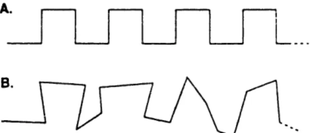
(i.e., not fractal) by perturbing a square wave (see Figure 2.4). Figure 2.5 gives the

log N vs. log r plot for this wave. The approximate straight line is suggestive of

scaling with D

=

1.11, which is clearly wrong by construction of the curve. Andrle

and Abrahams (1989) then plot apparent length L

=

Nr versus r (reproduced in

Figure 2.6) which for a fractal should satisfy

La rl

_(2.32)

I I II I I r I 1

_

I

i

i

K...

Figure 2.4. Sections of (A) a regular square-wave form and (B) a randomized square-wave form. (from Andrle and Abrahams, 1989)

10000 -o 1000-100 10 -W sn 01t 67 7,n 3,, i I i I I 0 1 1 0 10 100 lo000 0000 Steplength, G (units)

Figure 2.5. Graph of number of divider steps against steplength for the randomized square-wave form. Numerals on the graph indicate the number of superimposed points. (from Andrle and Abrahams, 1989)

0 C -J 5 £r S S Se UO C 200o-wm, 776 1763' 1c' 31777C'1,i 0.1 130 10 100 1000 10000 Steplength, G (units)

Figure 2.6. Graph of measured length against scale of measurement for the randomized square-wave form. Numerals on the graph indicate the number of superimposed points. (from Andrle and Abrahams, 1989)

I

I 1 -1

curve of Andrle and Abrahams (1989). The principle of plotting apparent measure L

= NrD versus r with D obtained from the N vs. r plot appears to be a good one, as a check for breaks in scaling. The apparent measure should be a constant function of r.

Box counting uses the fact that the number of boxes of side r, needed to cover a fractal set S is theoretically

Nbox(r) x r- D (2.33)

Therefore, the slope of log N vs. log r plots give estimates of D.

Indirect methods of measuring D include use of variograms and spectral densities. Voss (1986) gives ways to relate variogram (difference) scaling exponents and spectral scaling exponents to fractal dimension D.

Goodchild and Mark (1987) review the application of fractal models in geography. Here we will just focus on two aspects, the land surface and the channel network.

Mandelbrot (1977) found that many natural lines, such as coastlines, contours, political boundaries (sometimes consisting of rivers or coastlines), etc., seemed to have fractal dimensions near 1.2 - 1.3. He also noted that simulations of fractional brownian surfaces with D L- 2.3 looked remarkably like the real landscape. He took this as evidence that landscapes were fractal characterized by D L 2.3. The relationship between the fractal dimensions of a surface and a line projected from the surface (e.g., contour or profile) is

D1 = Ds -1 (2.34)

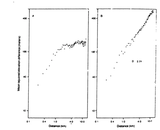
Mark and Aronson (1984) used variogram techniques to estimate the fractal dimension of the land surface of 17 USGS 7.5 min quadrangles from digital elevation data. Sixteen of these showed some evidence of characteristic scales at which fractal dimension changed, often sharply. Over short scales (below 0.6 km) they found that many surfaces do indeed resemble fractional brownian surfaces with dimensions of around 2.3. At larger scales however many areas were characterized by much higher dimensions, around 2.75. Ahnert (1984) notes the relationship

R ~ LH (2.35)

with exponent H L- 0.8. Here R is local relief (difference in elevation) in an area with diameter L. Ahnert (1984) attributes the log slope of 0.8 to a morphological expression of the dynamic equilibrium between the maximum geophysically possible rate of long-term uplift and the denudational response. Culling (1986) notes that this is analogous to a Hurst phenomenon (i.e. the persistence in long term hydrologic time series, noted by Hurst (1951)) in the landscape, and as such characterizes the landscape as scaling with fractal dimension

D = 3 - H (2.36)

For further information on the Hurst phenomenon, a feature of long-term hydrologic time series, see Bras and Rodriguez-Iturbe (1985). Culling and Datko (1987) also look at scaling in the landscape. They claim to predict theoretically, although the basis for the predictions is not clear from their paper, that:

* The Hausdorf dimension of soil slopes governed by a diffusion degradation regime will take values between 2 and 2.3 tending towards the lower value as diffusion proceeds.

*

The landscape will show evidence of a second fractal structure

associated with the drainage network with fractal dimension between

2.4 and 2.6.

*

The dimension of a level set (intersection with horizontal plane, i.e., a

contour) or vertical set (intersection with vertical plane, i.e., a profile)

is one less than that of the parent surface [i.e., consistent with

Equation 2.34)].

Culling and Datko present results from 17 1:25,000 ordinance survey maps in

southern England. The intersection of mapped contours with lines traversing the

sheets diagonally was used to produce profiles. The fractal dimension of the profiles

were estimated using the ruler method and variogram techniques. For many of

these data sets two different fractal dimensions are quoted, presumably from two

distinct slopes at different scales. Although Culling and Datko (1987) do not discuss

it, their Figure 6 [reproduced here, Figure 2.7] has similar sharp breaks in scaling

to those discussed by Mark and Aronson (1984) [Figure 2.8], with different fractal

dimension above and below the characteristic scale determined by the break in

scaling.

The above studies suggest that the domains with different fractal dimensions

could be interpreted in terms of different geomorphological processes operating or

dominating at different scales. Goodchild and Mark (1987) point out that most real

geomorphological entities are not pure fractals in the sense of having a constant D,

but in a lesser sense of exhibiting the behavior associated with a fractional

dimension over some range of scales. D thus provides a characteristic parameter

whose variation can be usefully interpreted in terms of the important processes over

the range of scales for which D holds constant.

Ln

Ln r

Figure 2.7. Burwash TQ 62. Richardson plots for 300' and 400' contours. (from Culling and Datko, 1987)

B

f

Figure 2.8. Variograms for the Aughivick. Pennsylvania (A) and Shadow mountain, Colorado (B) digital elevation models. Each point represents the mean squared elevation difference for points within a certain distance class. Total sample size was 32,000 pairs of points: distance classes with fewer than 64 pairs have been omitted from the diagram. (from Mark and Aronson, 1984)

S _,-E 100 a, 40 1 a' S 10 40 1O0

Eagleson (1970, p. 379) presents data from several studies that support the relationship first suggested by Hack (1957)

L=kAa _(2.37)

where L is mainstream length and A basin area. k and a are coefficients, typically k

= 1.4 and a = 0.57. Dimensional consistency and geometric similarity would

suggest that a should be 0.5. Mandelbrot (1977; 1983) uses this result to suggest that rivers are fractals with dimension 2a L 1.1 or 1.2. Mandelbrot (1983) also describes some fractal geometric patterns that resemble river networks where the fractal dimensions of individual lines is 1.1 but the complete network is space filling with D = 2. He suggests that these patterns are models of river networks. Hjelmfelt (1988) uses the ruler method in eight individual streams in Missouri and estimates fractal dimension near 1.1.

La Barbera and Rosso (1989) and Tarboton, et al. (1988) siaw that for river networks that obey Horton's laws, the fractal dimension is given by

log Rb

D log Rb Rb > R (2.38)

=1 _{Rb < RI}

In practice Rb > R, always holds. They use measurements of Rb and R• to estimate D and find D for the whole network ranging from 1.5 to 2.

This fractal dimension of river networks clearly can only apply at scales where we have a network. This may be all scales if we use the generalization of Davis (1899) given above or more likely it may be above a threshold scale related to the drainage density. Church and Mark (1980) discuss the relationship between

total length of channels and area. They note that below a certain threshold, a finite

drainage area may have no channels. Above this threshold they use data from

Wood and Snell (1957) to show that total length (LT) is proportional to area (A),

supporting the idea that drainage density (defined in equation (2.7)) is independent

of area

.

Above the threshold, LT could be used as a surrogate measure for A,

suggesting that the total length behaves or scales the same as area, and therefore

should have the same fractal dimension, i.e., be space filling with D

=

2.

A series of papers (Goodchild, et al., 1985; Goodchild and Mark, 1987;

Goodchild, 1988) investigates drainage networks on fractional brownian (fbm)

surfaces. They note that networks on fbm surfaces show similar deviations from

topologic randomness to those noted by Abrahams (1984). This supports the notion

that these deviations are due to the geometric constraints imposed when basins

must pack together on a surface, a space filling constraint. The abundance of pits

(areas that do not drain) on fbm surfaces casts doubt on the generality of these

results and the suitability of fbm as a model for terrain. However Goodchild (1988)

suggests that if pits are assumed to fill as lakes, fbm may be a useful model for

lake-rich landscapes.

2.7 Channel Network Evolution and Processes

It is important when considering channel network and landscape geometry to

have an appreciation of the processes that have and are continuing to sculpt the

landscape. Ultimately we want to understand the relationship between form and

processes and be able to make quantitative statements about the processes from

detailed analysis of the form. Hydrologists are particularly interested in the runoff

processes and movement of water and their excursion into geomorphology is from a

need to address the problem of prediction from ungauged basins and an attempt to

deduce processes from land form and channel network morphology. This section

will review the literature in geomorphological processes restricting ourselves to work that we feel is relevant. There is no attempt at completeness.

There is general agreement that elevation in channel networks and hillslopes may be thought of as an "open dissipative system" (Leopold and Langbein, 1962; Scheidegger, 1970; Thornes, 1983; Huggett, 1988). Carson and Kirkby (1972) provide a good review of the early work on evolution of hillslopes, relating form to processes. The formalism of differential equations describing the landscape surface is useful. Kirkby (1971) and Smith and Bretherton (1972) give the equation describing conservation of sediment as

= - V • F _(2.39)

where z is elevation and F is the sediment or debris flux vector. With the reasonable assumption that this flux is in the direction of steepest gradient, Smith and Bretherton (1972) write

F=Fn

where

Vz

is a unit downslope vector, and F is the magnitude of the sediment transport flux, per unit contour width, a scalar field, With this

= V F (2.40)

Smith and Bretherton (1972) further assume F(S,q), i.e., F is a function of the slope

S

=

I Vz

and flow of water q. The water flow is assumed to be a function of the

area draining through unit contour width a with drainage in the steepest direction.

Thus we can write F(S,q(a))

=

F(S,a), with a, a field which by continuity obeys

V n a = -1 (2.41)

Note that in the context of hillslopes lower case a is used to denote area per unit

contour width, a two-dimensional scalar field, while in the context of channel

networks A denotes total contributing area. A is thought of as concentrated, i.e.,

flowing through a point with width neglected. When using digital elevation data,

unit width is taken as the pixel size so the two notions of area are numerically

equivalent. Smith and Bretherton (1972) carry out a linear stability analysis of

Equation (2.40) and (2.41) and show that the pair of equations is unstable in the

sense that small perturbations grow when

F- a

₀

_(2.42)

Smith and Bretherton (1972) also show that a one-dimensional equilibrium or

constant form solution is concave when Equation (2.42) is satisfied and convex

otherwise.

There is therefore an equivalence between concavity of a

one-dimensional profile and instability in the two-dimensional landscape.

Instability as characterized above would lead to rilling and channel growth.

Otherwise, smooth hillslopes would prevail.

Luke (1972, 1974) generalizes the Smith and Bretherton (1972) formulation.

Instead of assuming F(S,q), which assumes the sediment load is always in

equilibrium with slope, he suggests an additional equation

(2.43)

;7= - f(S,q,F)

The function f(.) will be such that when the sediment load F is small, f(.) is positive, i.e., erosion, whereas when F is large, f(.) will be negative, i.e., deposition.

Luke (1974) shows how the basic equations (2.40), (2.41), and (2.43) can be solved using the method of characteristics. He also shows how under conditions of instability troughs develop into shock discontinuities, interpreted as channels.

The behavior of Equation (2.42) is clearly dependent on the form of the sediment transport flux function F(S,a). A common form is (Kirkby, 1971)

F oc am Sn (2.44)

Table 2.1 excerpted from Kirkby (1971) gives typical m and n for various processes.

Table 2.1

Typical Values of Exponents m and n in the empirical relationship F (o am Sn (Equation (2.44)

Process m n Sources

Soil creep 0 1.0 C. Davison, 1889; Culling,

1963

Rainsplash 0 1-2 Schumm, 1964

Soil wash 1.3-1.7 1.3-2 Musgrave, 1947; U.S.

Agric. Res. Serv., 1961; Zingg, 1940; Kirkby, 1969

Rivers 2-3 3 Derived from Leopold and

Maddock, 1953 (from Kirkby, 1971)

Kirkby (1971) studied the solution to Equations (2.40) and (2.41) in one dimension and identified characteristic profiles under different assumptions for the sediment transport F (Equation 2.44). These are reproduced in Figure 2.9 and show

0-8 S0-6 0-4 0-2 n 0 0-2 0-4 0-6 0-8 1-0 x/x1

Figure 2.9. Characteristic form slope profiles. (from Carson and Kirkby, 1976) k.