HAL Id: hal-01413811
https://hal.archives-ouvertes.fr/hal-01413811
Submitted on 15 Dec 2016HAL is a multi-disciplinary open access archive for the deposit and dissemination of sci-entific research documents, whether they are pub-lished or not. The documents may come from teaching and research institutions in France or abroad, or from public or private research centers.
L’archive ouverte pluridisciplinaire HAL, est destinée au dépôt et à la diffusion de documents scientifiques de niveau recherche, publiés ou non, émanant des établissements d’enseignement et de recherche français ou étrangers, des laboratoires publics ou privés.
Detecting Climatic Signals from Ship’s Datasets
Pascal Terray
To cite this version:
Pascal Terray. Detecting Climatic Signals from Ship’s Datasets. INTERNATIONAL WORKSHOP ON DIGITIZATION AND PREPARATION OF HISTORICAL MARINE DATA AND METADATA, World Meteorological Organization and National Oceanic and Atmospheric Administration (NOAA, USA), Sep 1997, Tolède, Spain. pp.83-88. �hal-01413811�
Detecting Climatic Signals from Ship’s Datasets
Pascal TerrayLaboratoire d’Oceanographie Dynamique et de Climatologie, Paris, France 1. Introduction
Marine ship observations over the vast oceanic regions are crucial to studies of climate variability on timescales from the seasonal to multidecadal. However, any climatic analysis of this historical record is hampered by two difficult problems, namely:
• The systematic instrumental errors which contaminate the ship observations. For example, it is well-known that most of the ship-reports before 1940 contain a large majority of uninsulated b u c k e t S e a S u r f a c e T e m p e r a t u r e ( S S T ) measurements which are biased low, while the data after the 1940s are mostly injection or insulated bucket SST measurements which are biased high (Bottomley et al., 1990).
• The irregular space-time sampling of the ship-reports. For example, COADS summaries provide meteorological variables in the form of monthly means for 2
°
x 2°
latitude-by-longitude cells (Woodruff et al., 1987). In such datasets, the number of observations used to compute a particular monthly mean reflects the number of ships that cross the box that month. Thus, for a particular month, one cell’s mean may be computed from hundreds of observations, while others may be based on only a few, and there may be many cells with missing means due to the poor spatial and temporal coverage outside the main shipping lanes.The former problem is particularly relevant to studies of multidecadal variability, and has led researchers to design instrumental correction procedures for the meteorological and oceanic fields derived from ship-reports and used for assessing climatic changes, e.g. SST and wind.
The latter problem attends almost all climatic studies from seasonal to multidecadal timescales, but is particularly relevant to the interannual to multidecadal. The classical solution to cope with this problem is to use some kind of objective analysis. This technique spatially smooths the oceanic fields by filling the data-void areas with reasonable values which are a linear combination of climatology and anomalies observed in the neighborhood of each grid’s cell. The drawbacks of this solution are: First, the need for a very good climatology which has to be constructed before the analysis. Second, the oceanic fields derived from objective analysis are
generally over-smoothed with the undesirable consequence of a decrease in the spatial resolution of the data.
The main objective of this work is to present a new multivariate statistical method to deal with this last problem. The method may be termed weighted Empirical Orthogonal Function (EOF) analysis or weighted Singular Value Decomposition (SVD) analysis and is a generalization of the traditional EOF analysis, or more precisely, of truncated SVD analysis. This method accounts for the irregular space-time sampling of the ship-reports by the use of weights (a weight is associated with each cell-month entry of the data matrix) in approximating the data matrix by a lower rank matrix in the least squares sense. In contrast, the traditional SVD analysis assumes that all the cells have equal weights in solving the same optimization problem.
The organization of this paper is as follows: first, the formalism of the weighted SVD analysis is presented and its relationships to traditional SVD analysis are outlined. Second, we illustrate with some examples how weighted SVD analyses are useful for extracting seasonal, interannual and multidecadal climatic signals from ship’s datasets such as COADS summaries. Finally, we highlight the utility of the weighted SVD analysis for different common tasks in meteorology and oceanography.
2. Theory
The widespread acceptance of EOFs for data reduction purposes, to aid in determining the variability of oceanic and atmospheric fields, or to identify coherent modes of atmospheric parameters suggests that the adaptation of this method to ship’s datasets can provide us an improved tool to extract climatic signals from such noisy data. However, traditional EOF analysis is not well-adapted to ship’s datasets since the method gives the same weight to all the data matrix entries without taking account of the irregular space-time sampling of the ship’s reports when determining eigenvectors and principal components. Moreover, it is impossible to compute EOFs if some data are missing.
By contrast, the new method of analysis we will develop takes directly into account these uncertainties of the data while estimating the EOF model. In order to introduce this new method, it is first useful to review some of the optimal properties of traditional EOFs
(Kutzbach, 1967). This is a necessary step to understand the new method.
Let X denote an p x n data matrix consisting of
n time observations (columns of X) for p grid cells or
stations (rows of X). In the complete case, where X is a full matrix with no missing values, the “full EOF model” can be expressed as a matrix product, where E is an p x p orthogonal matrix, whose columns are the eigenvectors of the p x p symmetric matrix,
If the data are centered in rows, this last matrix is simply the covariance matrix between the grid’s cells. Furthermore, the elements in the i’th row of C represent time variations associated with the i’th eigenvector.
One of the most important optimal properties of EOFs, especially for data reduction purposes, is that maximum inertia of the data matrix is explained by choosing in order the eigenvectors associated with the largest eigenvalues of R.
More precisely, it can be shown that the fraction of the total inertia, Vk, explained by the eigenvectors associated with the k largest eigenvalues can be obtained from
In the application of EOFs to highly correlated fields such as those commonly analyzed in meteorology, this means that a large portion of inertia can be accounted for by retaining only the first few eigenvectors. This leads to define a “restricted k EOF model” to approximate and to study the data: where E.kstands for the first k columns of E, and similarly Ck. designates the first k rows of C.
The optimal properties of EOFs can be stated directly in terms of this restricted EOF model as follows: the k-component model forms an optimal approximation to the original matrix in the sense of least squares. That is, the minimum of
on all p by k matrix A and all k by n matrix B is obtained by taking E.kand Ck.as A and B, respectively. Moreover, this minimum is equal to
Now let X denote a typical ship’s dataset such as COADS 2
°
lat x 2°
long trimmed monthly means for some area and historical period. In order to take into account the sampling properties of this ship’s dataset while estimating a restricted k EOF model, we may correspondingly seek a minimum ofon all p by k matrix A and all k by n matrix B.
Here, W is an p by n positive weight matrix constructed in such a way that the resulting EOFs and principal components are defined to emphasize the better-observed aspects of the data. In particular, for the extreme case of zero sample size, an entry of the data matrix should play no role in fitting the model; this can be done by assigning zero weights to such cells.
There are several ways to determine this weight matrix in order to take into account that the monthly means for each grid cell are based on samples of widely varying sizes:
a) The simplest method is to set = 1 if is present = 0 if is missing
This will take care of missing values, but gives the same weight to all non-missing cells in the data matrix.
b) Another choice is to fit the k EOF model with weights proportional to size samples where is the number of ship observations contributing to the cell’s monthly mean .
c) A more elaborate strategy is to use some smooth function of the number of observations = 1 – exp where again is the number of ship observations used in computing . For this particular weight function, is in the neighborhood of 1 if >10 and near 0.5 if
equals 6.
d) Still another strategy for constructing the weight matrix is to use the inverse of the variance or standard error associated with each grid’s cell and month. This information is, for example, available in the distribution files of COADS (Woodruff et al., 1987).
After the weight matrix is constructed, we have to minimize the least-squares problem stated above in order to estimate the EOFs and their associated principal components. Note that this cannot be done by solving some eigensystem as in the traditional EOF analysis, and we have to use non-linear least-squares techniques (Gauss-Newton or Marquardt-Levenberg algorithms) to obtain a solution to our problem. The algorithms used X = E
⋅
C ET⋅
E = Ip R 1 n ---⎝ ⎠ ⎛ ⎞ X X(
⋅
T)
= Vk λl l= 1 k∑
λl l=1 min p n( , )∑
÷ = X≈
E.kCk. X–(
A⋅
B)
2 Xij AilBlj l= 1 k∑
– ⎝ ⎠ ⎜ ⎟ ⎜ ⎟ ⎛ ⎞2 ij∑
f A B( , ) = = λl l=k+1 min p n( , )∑
f*(A B, ) Wij Xij AilBil l= 1 k∑
– ⎝ ⎠ ⎜ ⎟ ⎜ ⎟ ⎛ ⎞2 ij∑
= Wij Xij Wij Xij Wij = αNij Nij Xij Wij Nij⁄6 – ( ) Nij Xij Wij Nij Nijhere to minimize f*(A,B) are a generalization of the techniques described in Terray (1995). Once this is done, the last step is to compute the SVD of the product in order to normalize the solution as in the traditional EOF approach. This new method will be referred to as weighted EOF analysis in the rest of this paper.
3. Examples
In order to illustrate the application of this technique and to show that this method allows us to analyze the natural variability exhibited by data of varying reliability, two classical ship’s datasets were analyzed using the weighted EOF technique.
Example 1
The first example is a weighted EOF analysis of the January 1993 version of the Global Ocean Surface Temperature Atlas (GOSTA; Bottomley et al., 1990). The data in this atlas are presented as monthly anomalies on a 5
°
latitude x 5°
longitude grid wherever data existed. The data were extracted for the period from 1900 to 1991. The weight function used in this analysis is simply: = 1 if is present and = 0 if is missing. Note that this is not a very good choice since this will give the same weight to all non-missing data, but there is no information on the number of ship-reports used to compute monthly anomalies for individual grid cells in the distribution files of GOSTA.With this weight function, a two-component model was estimated. At the end of the iterations, the two-component model explains a little less than 16% of the total weighted inertia of the data. Note that the norm of the gradient of the objective function has been decreased by several orders of magnitude from the initialization to the end of the algorithm.
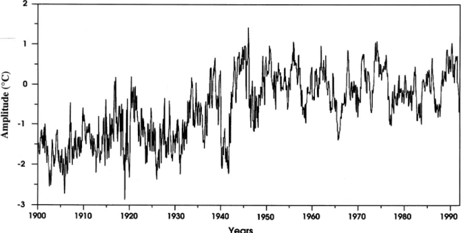
The first estimated principal component is shown in Figure 1. This time series as presented has unit variance. The associated eigenvector is shown in Figure 2. This eigenvector has been multiplied by the square root of its associated eigenvalue. In this way, the spatial loadings depicted in Figure 2 can be interpreted as covariance coefficients between the grid’s cells and the time series plotted in Figure 1.
Interdecadal changes of SST are particularly evident in this first principal component. The time series suggests a cold start of the twentieth century with a sudden warming between about 1920 and 1940. After World War II, the time series suggests a slight cooling until 1976. After this date, a slow but regular warming took place. Indeed, this first estimated principal component is very similar to the time series of global and
hemispheric temperature anomalies presented by Parker et al. (1994). However, an important discrepancy between our time component and the estimates of Parker et al. is that recent decades are not substantially warmer than the preceding ones on Figure 1.
Note also that the first part of this time series is much more noisy than the last part; this may be due to our choice of the weight function since we gave the same weight to all data entries with non-missing values in the atlas without taking account of the number of ship-reports used to construct the anomalies. In the same fashion, the strongly negative time coefficients during World War II are due to high and isolated positive monthly anomalies in the central and eastern Pacific which were likely computed using very few ship observations. We hypothesize that a much better job can be done about these two problems if we use a more appropriate weight function.
The spatial pattern associated with this time series suggests that these decadal SST variations are well-marked in the midlatitude North Pacific and in parts of the middle-to high-latitude Southern Ocean (Figure 2). By contrast, the areas in the central and eastern equatorial Pacific and also in the South Indian Ocean are negatively correlated to this time series. It may be pointed that this fact is also evident in the global fields of decadal annual surface temperature anomalies presented by Parker et al. (1994).
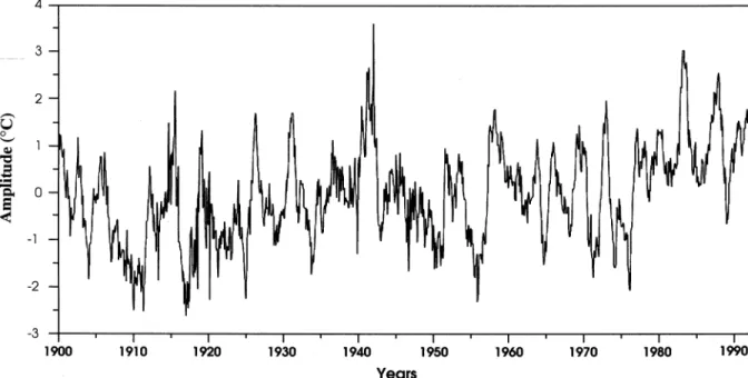
The second estimated principal component is shown in Figure 3. A strong interannual signal seems to be present in this time series with a time-scale of about 3 to 4 years, especially in recent decades. A sudden warming may also be noticed after 1976. The estimates during World War II are again unreliable.
The spatial loadings associated with this time series exhibit the well-known ENSO signature with a warm tongue in the central and eastern Pacific, and with smaller amplitudes and opposite phase in the middle latitude North and South Pacific (Figure 4). Some positive areas also are noticeable in the Indian Ocean. Thus, this second principal component and its associated spatial pattern suggest that recent warmings may have some connections with ENSO and a sudden change of the climate mean state which took place in the pacific regions during 1976.
A
⋅
BFigure 1: GOSTA global SST missing SVD analysis (rank=2). Estimated SST EOF1 amplitude.
Figure 3: GOSTA global SST missing SVD analysis (rank=2). Estimated SST EOF2 amplitude.
Example 2
The second example is taken from the COADS trimmed monthly mean summaries (Woodruff et al. 1987). SSTs over the Indian Ocean (41
°
S-31°
N and 29°
-121°
E) were extracted for the period 1900 to 1992. Note that these data are not anomalies but estimates of monthly mean SST on a 2°
latitude x 2°
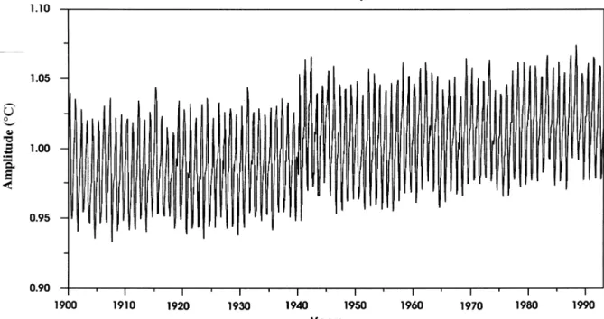
longitude grid.The weight matrix used in this analysis was constructed with the smooth function of the number of observations contributing to each cell’s monthly mean value discussed in Section 2. Again, a two-component model was estimated from the data by the weighted EOF technique. These two components explain more than 99.8% of the total weighted inertia.
The first principal component is, to a very good approximation, sinusoidal with an annual period (Figure 5). An interdecadal trend seems also to be present in this time series with a sudden warming after 1976. The same results may be obtained by averaging the data for the whole Indian Ocean (Terray, 1994). The associated spatial pattern exhibits a north to south gradient of SST (Figure 6). Note also that SST is colder off the African coast.
The second principal component (not shown) is still marked by an annual period but its spatial pattern shows a characteristic phase difference between North
and South which adds an annual modulation to the first principal component and its associated eigenvector.
In order to present in a more traditional manner the annual signal described by these two time series and their associated spatial loadings, a climatology of Indian Ocean SSTs was computed from the rank 2 weighted approximation of the data given by the two-component model. This climatology may then be compared to a traditional climatology obtained from an objective analysis in order to show the coherence of the results.
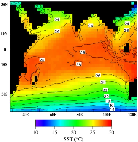
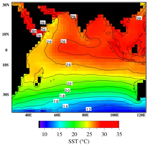
The mean SST fields for January and July obtained from the rank 2 weighted approximation of the data are shown in Figures 7 and 8.
SST patterns in the January mean field are dominated by highest temperatures (28
°
C) in the eastern Indian Ocean between the equator and about 15°
S and also near Madagascar. Strong SST gradients are evident over the higher latitudes of the southern Indian Ocean.The July mean SST fields show the effect of upwelling and monsoon cooling near the African coast associated with the Somali jet and to the south of Peninsular India while other parts of the North Indian Ocean are still dominated by warmer SST. All these patterns are found in classical atlases (Hastenrath and Lamb, 1979; Bottomley et al., 1990).
Figure 6: Indian Ocean SST estimated EOF1 (98.6%, rank=2).
Figure 7: SST mean (COADS) January.
2 8 2 6 14 1 6 1 8 20 22 2 4 2 6 2 6 2 8
40E 60E 80E 100E 120E
30S 10S 0 10N 30N
10
15
20
25
30
SST AMPLITUDE (°C)
16 24 2 6 2 6 24 2 6 2 8 2 8 2 8 2 6 24 22 2 0 1 8 1 440E 60E 80E 100E 120E
30S 10S 0 10N 30N
10
15
20
25
30
SST (°C)
Figure 8: SST mean (COADS) July. 28 1 2 1 4 3 0 28 28 28 1 6 1 8 2 0 22 2 6 2 6 28 28
40E 60E 80E 100E 120E
30S 10S 0 10N 30N
10
15
20
25
30
35
SST (°C)
4. ConclusionsEOF analysis has been widely used to explore the spatial and temporal relationships within large geophysical datasets. This success can be explained by the ability of EOFs to compress the main modes of variability in the original dataset into a few time series and associated spatial patterns. Indeed, the EOF technique can be thought of mathematically as a method for approximating data matrices by matrices of lower rank since conventional EOFs provide the best approximation of a data matrix in the sense of least squares under the assumption that all the data entries have the same weight equal to one.
This paper presents an extension of conventional EOFs when weights are assigned to data entries in the original dataset. The new method which may be termed weighted EOF analysis is designed to fit a lower rank least squares approximation to a data matrix with a general choice of positive weights. If the weight matrix is carefully constructed, this new tool allows us to analyze the natural variability exhibited by data of varying reliability. It must also be emphasized that the
proposed method directly takes care of missing values by assigning zero weights to such data entries.
Indeed, there are many situations in which weighted EOF analysis is more appropriate than conventional EOFs. In particular, weighted EOF analysis is shown to be a useful tool for extracting climatic signals from ship’s datasets which are characterized by a strong irregular space-time sampling. In the context of ship datasets with irregular space-time sampling, weighted EOF analysis can be particularly useful for the following purposes:
• accurate and robust detection of climate signals (annual, interannual and multidecadal) on a grid-mesh, directly from the ship observations;
• blended analysis of marine and land datasets; • interpolation of missing values;
• derivation of climatologies and smooth oceanic fields;
• sensitivity experiments (e.g. by using various weight matrices with the same dataset).
Other applications of weighted EOF analysis will be reported in detail elsewhere.
References
Bottomley, M., Folland, C.K., Hsiung, J., Newell, R.E., and Parker, D.E., 1990: Global ocean surface
temperature atlas “GOSTA”. Joint project of the UK
Meteorological Office and Massachusetts Institute of Technology, 20 pp., 313 plates, HMSO.
Hastenrath, S., and Lamb, P.J., 1979: Climatic atlas of
the Indian Ocean. Part I: Surface climate and atmospheric circulation. The University of Wisconsin
Press, Madison, 109 pp.
Kutzbach, J.E., 1967: Empirical eigenvectors of sea level pressure, surface temperature, and precipitation complexes over North America. Journal of Applied
Meteorology, 6, 791-802.
Parker, D.E., Jones, P.D., Folland, C.K., and Bevan, A., 1994: Interdecadal changes of surface temperature since the late nineteenth century. Journal of
Geophysical Research, 99 (D7), 14,373-14,399.
Terray, P., 1994: An evaluation of climatological data in the Indian Ocean area. Journal of the Meteorological
Society of Japan, 72, 359-386.
Terray, P., 1995: Space-time structure of monsoon interannual variability. Journal of Climate, 8, 2595-2619.
Woodruff, S.D., Slutz, R.J., Jenne, R.L., and Steurer, P.M.,1987: A Comprehensive Ocean-Atmosphere Data Set., Bulletin of the American Meteorological