Complexity of two-dimensional quasimodes at the transition from weak scattering to Anderson localization

HAL Id: hal-00432887

https://hal.archives-ouvertes.fr/hal-00432887

Submitted on 8 Dec 2009

HAL is a multi-disciplinary open access

archive for the deposit and dissemination of

sci-entific research documents, whether they are

pub-lished or not. The documents may come from

teaching and research institutions in France or

abroad, or from public or private research centers.

L’archive ouverte pluridisciplinaire HAL, est

destinée au dépôt et à la diffusion de documents

scientifiques de niveau recherche, publiés ou non,

émanant des établissements d’enseignement et de

recherche français ou étrangers, des laboratoires

publics ou privés.

Complexity of two-dimensional quasimodes at the

transition from weak scattering to Anderson localization

Christian Vanneste, Patrick Sebbah

To cite this version:

Christian Vanneste, Patrick Sebbah. Complexity of two-dimensional quasimodes at the transition

from weak scattering to Anderson localization. Physical Review A, American Physical Society, 2009,

79, pp.041802. �10.1103/PhysRevA.79.041802�. �hal-00432887�

1_{Laboratoire de Physique de la Mati`ere Condens´ee/CNRS UMR 6622/Universit´e de Nice - Sophia Antipolis,}

Parc Valrose, 06108, Nice Cedex 02, France (Dated: March 12, 2009)

Quasimodes of an open finite-size two-dimensional (2D) random system are computed and systematically characterized in terms of their spatial extension, η, complexity factor, q2_{, and phase distribution for a random}

collection of systems ranging from weakly scattering to localized. A rapid change is seen in η and q2_{at the}

transition from localized to diffusive which corresponds to the emergence of 2D extended multipeaked quasi-modes analogous to the necklace states recently observed in 1D. These 2D quasiquasi-modes are interpreted in terms of coupled localized states.

PACS numbers: 42.25.Dd, 42.55.Zz

Transport in random media is driven by the nature of the underlying eigenmodes. Propagation is diffusive when the modes extend spatially, while spectral level overlap occurs in transmission spectra. As the degree of the overlap decreases, transport is inhibited and modes become spatially localized [1]. The theory of Anderson localization predicts a transi-tion between localized and extended eigenstates for spatial dimensions larger than two [2]. Renewed interest in the lo-calization transition has been boosted by the active ongoing search for localization of Bose-Einstein condensate in laser speckle fields [3, 4], the recent observations of the slowing down of diffusion in ultrasounds [5], microwave [6] and time-resolved optical [7] experiments, and new theoretical pro-gresses [8, 9] towards an analytical description of the metal insulator transition (MIT). The question of the spatial extent of the modes near the Anderson transition is also central in random lasers [10, 11]. The threshold may vary by orders of magnitude between localized systems where the modes are spatially confined and diffusive systems where the modes are extended. Besides their spatial extent, another property of the modes in open random media is their complexity. As their spatial extent is increased up to the sample dimensions and their linewidth broadens with increasing leakage through the boundaries, the decaying quasimodes or resonances, which generalize the concept of mode to leaky systems [12], be-come complex-valued, their standing wave component being progressively replaced by a component traveling toward the opened boundaries [13]. This is analogous to chaotic cavities with an increasing degree of opening [14]. This is an impor-tant aspect rarely addressed in the context of random media.

In this paper, we use numerical simulations to explore the nature of the quasimodes of 2D open random media when scattering strength is increased. The spatial extension of the computed quasimodes, their complexity factor and their phase distribution are calculated for a statistical ensemble of random configurations for each value of the scattering strength. These quantities reveal the change of regime and the transition from diffusive to localized. A detailed analysis of the phase prob-ability distribution for each mode shows multipeaked wave-functions in the vicinity of the transition when the

localiza-tion length is comparable to the sample size. These extended multipeaked quasimodes are interpreted in terms of coupling of localized isolated states, which hybridize to form 2D neck-lace states.

We consider a two-dimensional random collection of paral-lel dielectric cylinders with infinite extension, radius r = 60 nm and refractive index n, embedded in a background ma-trix of index 1. Volume fraction is φ = 40 % and system size is L2 _{= 5x5 µm}2_{. Maxwell equations for TM polarization}

are modeled using the finite-difference time-domain method [15]. Open boundary conditions are approximated by per-fectly matched layer (PML) absorbing boundaries [16]. The index of refraction n is varied from 1.05 to 2.0, in step of 0.05, corresponding to scattering mean free path ranging from 50

µm to 0.1 µm. For most of this range, modes are short lived

with strong spectral overlap, preventing individual excitation of a mode at its eigenfrequency by a monochromatic source. To obtain the wavefunction of such short lived-modes, we use recent results [17] which show that, when operating just above threshold, the first lasing mode of an active random system corresponds to a quasimode of the passive system, even in weakly scattering systems where modal overlap dominates. Introducing gain and adjusting the pumping rate just above threshold is therefore an alternative to select a quasimode of the passive cavity. To model the gain, we couple the popula-tion equapopula-tions of a four level atomic system to the Maxwell equations via the polarization equation [18]. The gain natu-rally selects the mode with the longest lifetime and the best spectral overlap with the gain curve. All the parameters and initial conditions used here have been already fully described in [19].

We study 150 random configurations, 10 on average per value of refractive index, n. The amplitude and phase spatial distributions of the mode are obtained by integrating the in and out of phase oscillating fields over a period. Examples of spatial distributions of the magnitude are shown in Fig. 1 for decreasing values of the refractive index, n, illustrating differ-ent degrees of spatial extension of the wavefunctions within the system. The corresponding phase probability distributions between 0 and 2π are shown in insets in Fig. 1. The phase

dis-2 0 0.2 0.4 0.6 0.8 1 0 0.1 0.2 0.3 0.4 0.5 0.6 0.7 0.8 0.9 1

n=1.05

447.2nm

n=1.25

447.1nm

n=1.50

445.4nm

n=1.75

445.7nm

n=1.85

447.1nm

n=2.00

447.9nm

FIG. 1: Spatial distribution and wavelength of quasimodes corre-sponding to decreasing values of the refractive index of the scatter-ers, n=2.00 to n=1.05 (random configurations are not necessarily identical). All modes are in a narrow spectral range around the max-imum of the gain curve, λ=446.9 nm. Each frame shows in inset the phase distribution between 0 and 2π of the corresponding quasi-modes. Note the double peaked distribution for n=1.85.

tribution is peaked around 0 and π when the mode is localized (n=2), while it is more uniformly distributed in the extended case. Note that for values of the refractive index as low as 1.05, scattering is weak and the field is rather concentrated at the edges of the system. In that case, residual reflection either at the boundaries or from the PML layers may not be negligible and may result in periodic patterns, similar to those of a Fabry-Perrot cavity, as seen in the bottom-right frame of Fig. 1. We checked that above n=1.10, this effect is insignifi-cant and lasing is solely due to multiple scattering within the system.

As the scattering strength is reduced, the spatial expansion of the eigenfunctions increases, as well as the their imagi-nary part resulting from leakage at the open boundaries. To quantify these two characteristics, the quasimodes are de-scribed in terms of their spreading factor, η, and their com-plexity factor, q2_{. We define the spreading factor as η =}

3/L4R R_{A(~r) ˜˜ A(~r}0_{)|~r − ~r}0_|2_d2_~rd2_r~0_{, where the field}

ampli-FIG. 2: Color online. Complexity factor (dots), q2 _and

spread-ing factor (circles), η, averaged over sample configuration versus scattering mean free path, `. The fluctuations around the average, ±hq2_{− hq}2_ii1/2_{are represented by the bars. Inset: Averaged}

com-plexity factor, q2 _{(dots), localization length ξ versus index of}

re-fraction, n, calculated from the averaged lasing threshold (crosses) and from independent scattering theory (full line where relevant (ξ ≤ L/2), dotted otherwise). The dashed line represents the mean free path, `. The horizontal dotted line correspond to ξ = L/2

.

tude A(~r) is normalized ˜A(~r) = A(~r)/[R R A2_(~r)d2_~r]1/2_.

The normalizing factor 3/L4 _{ensures that η is unity for}

uni-form distribution of the field amplitude. It measures the de-gree of spatial extension of the energy within the system alike the participation ratio for instance. However, due to the weighting factor |~r − ~r0_|2_{, it also enables us to}

distin-guish systems with spatial localization of energy inside the system, as in Fig. 1 for n=2, from concentration of energy at the boundaries of the system, as in Fig. 1 for n=1.05. Indeed, it can be less than 1 for spatially localized modes, or larger than 1 when energy is distributed near the system edges. This is reminiscent of distributed feedback lasers [20] where in the over-coupled regime (corresponding to η < 1), energy is concentrated inside the laser as a result of strong feedback from scatterers, while in the under-coupled regime (η > 1), energy is concentrated at the edges since the las-ing modes result from scatterlas-ing at the boundaries in order to maximize the gain volume [21]. The complexity factor,

q2 _{= hIm(Ψ)}2_i/hRe(Ψ)2_{i [22], or equivalently the phase}

rigidity, ρ = (1 − q2_{)/(1 + q}2_{) [23], were introduced in the}

field of quantum chaos to quantify the degree of complexity of the eigenmode, Ψ(~r) = A(~r)eiφ(~r)_{, and the mutual}

influ-ence of neighboring resonances [24]. The complexity factor varies from 0 for real standing wavefunctions -corresponding to a phase distribution peaked at 0 and π- to 1 for purely

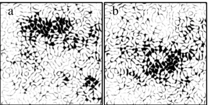
trav-FIG. 3: Binary plots showing in black where the phase is valued between (a) 0.89 − 0.99π and (b) 1.01 − 1.11π, i.e. two narrow phase ranges around the two peaks at 0.94π and 1.06π seen in phase distribution in the inset of Fig. 1 for n = 1.85.

eling waves -corresponding to a flat phase distribution. To the best of our knowledge, it has never been used as a probe to characterize the transition from localized to extended states in finite disordered systems.

The spreading factor and the complexity factor are com-puted for each mode and averaged over sample configurations for each value of n. They are shown in Fig. 2 as a func-tion of the scattering mean free path, `, calculated using Mie theory for infinite cylinders of refractive index n. The com-plexity factor increases with the mean free path, which means that the traveling wave component replaces progressively the standing wave component of the mode. While the complex-ity factor explores values between 0.06 and 0.78, it shows clearly two different regimes, with a crossover around `=0.14

µm corresponding to n=1.8. A transition occurs around the

same value of ` for the spreading factor, which ranges be-tween 0.16 and 1.23. This particular value of n certainly is not universal and depends on the sample size but it should correspond to a localization length, ξ, of the order of the sample size. We confirm this hypothesis by calculating ξ di-rectly from the value of the lasing threshold averaged over sample realizations, hP i. Indeed, the spectral width of the modes, Γ, resulting from leakage at the boundaries is given by Γ = Γ0·exp(−L/ξ) [25]. It is also directly proportional to the

lasing threshold, P , since at threshold, losses are compensated by gain. Therefore ξ = L/(lnhP0i − lnhP i),where hP i

des-ignates the average over sample configurations for each value of n and lnhP0i=20.15 is obtained by extrapolating hP i at n = 1. The dependence of ξ on refractive index, n, is shown

in the inset in Fig 2 and is compared to the theoretical expres-sion in the limit of independent scattering, as given in [25] by

ξth= ` exp[πRe(kef f)`/2], where ` is the mean free path and

kef f is the effective wavenumber. ”Both curves (full lines in

inset of Fig 2) approach in the crossover region around n=1.8, which corresponds to ξ ∼ L/2 =2.5 µm, where the two ex-pressions for ξ and ξthstart to be valid. [26]

Also shown in Fig 2 are the fluctuations of the complexity factor, ±hq2_{− hq}2_ii1/2_{. A significant increase of these}

tuations is seen at the crossover. We find that these large fluc-tuations are correlated with the occurrence of peculiar phase

the phase distribution at 0.94π and 1.06π. The spatial distri-butions of the phase for values comprised in a π/10 window around each of these two peaks are shown in Fig. 3a and b. These two distributions delimitate two distinct spatial regions associated with standing components of the mode, which os-cillate at the eigenfrequency of the mode but with a phase lag,

δφ = 0.12π. This phase lag suggests that this mode results

from the coupling between two distinct modes localized on each of the regions of Fig. 3. This would be the analog of the symmetric or anti-symmetric solutions to the coupled os-cillators problem in the presence of leakage which introduces a phase lag different from 0 or π between the components of the hybridized mode. To identify each of the two com-ponents of the double-peaked mode of Fig. 1 (n=1.85), we remove a scatterer in a spot where the field is high in one of the two regions displayed in Fig. 3 to selectively sepa-rate the two contributions. Each perturbed system is excited at the resonant frequency of the original unperturbed mode. The corresponding field distributions are shown in Fig. 4a and b. They reproduce the local features of each peak of the mode of Fig. 1, but extend far beyond. The corresponding phase distributions are now single-peaked. Note that layers of randomly distributed scatterers (not shown) were added at the boundaries of the perturbed system in order to increase the lifetime of the mode of Fig. 4a, which would be im-possible to excite otherwise due to its strong leakage. The resemblance between the normalized original mode, Ψ, and the normalized complex linear combination of the two modes of Fig. 4, Ψt = αΨa + eiφΨb, is measured by the spatial

cross-correlation,RR|Ψ||Ψt|d2~r, which is equal to 91% for

α = 0.78 and φ = 0.66π. The two quasimodes composing the

double-peaked state have also been identified by introducing gain in the perturbed systems. The wavelengths of the cor-responding lasing modes are λa=447.9nm and λb=446.8nm,

to be compared with λ=447.1nm (Fig. 1) for the original state. The linewidth of the passive modes are respectively

δλa=1.0nm, δλb=0.6nm, and δλ=0.8nm. The

correspond-ing spreadcorrespond-ing factors are ηa = 0.36, ηb = 0.29, η = 0.45.

This supports the picture of two coupled quasimodes with dis-tinct wavelengths, overlapping both spectrally and spatially, to form an hybridized double-peaked state. All other identified multipeaked quasimodes [27] (about 50% of the modes) arise around n=1.85, in the vicinity of the transition.

These multipeaked states are analogous to necklace states recently observed in nominally localized optical [28] and mi-crowave [29] one-dimensional layered systems. Modes over-lapping both in space and frequency may couple and form multipeaked extended states even in the localized regime [30]. Although scarce, they are predicted to play an outsized role in transport [31] in contrast to isolated localized states [32]. This is to be compared with the filament-like fractal picture of the modes at the transition suggested by Aoki [33]. Pendry ar-gued that the picture of 1D necklace states should generalize to 2D and 3D localized random media [31]. However, besides

4 0 6 1210 3 2π 0 φ P( φ ) 0 6 1210 3 2π 0 φ P( φ ) 446 449 λ (µm)

FIG. 4: Color online. Spatial distribution of the magnitude of the quasimodes together with their phase distribution (lower insets) for two different local perturbations of the original random system of Fig. 1 for n=1.85. The locations of the removed scatterers are shown by the circles. Upper inset: spectral lines of modes a (dots), b (circles) and mode n=1.85 in Fig. 1 (full line). Wavelengths and linewidths of the modes are given in the text.

earlier calculations in a percolation model, no observations of necklace states for classical waves in dimensions larger than one were reported [34, 35]. Our results point out to the exis-tence of necklace states in 2D and show that they should occur preferentially at the transition.

In conclusion, our numerical simulations provide with a de-tailed description of the quasimodes of open 2D random sys-tems ranging from weakly scattering to strongly localized in terms of their spatial extension but also for the first time in this context in terms of their complexity factor. We find mul-tipeaked quasimodes in the vicinity of a well-marked transi-tion between localized and extended states. Two mechanisms, which may coexist, were proposed to describe the transition [36]. The first one is a gradual spatial expansion of the mode as scattering strength is diminished, with a progressive in-crease of the localization length. Our results suggest a sec-ond mechanism, analogous to a percolation process, where the coupling of localized states lead to extended structures that form necklace states [37–39].

We thank D. Savin, O. Legrand and F. Mortessagne for fruitful discussions. This work was supported by the Cen-tre National de la Recherche Scientifique (PICS #2531 and PEPS07-20) and the Groupement de Recherches IMCODE.

∗ _{Contact: vanneste@unice.fr}

[1] D. J. Thouless, Phys. Rev. Lett. 39, 1167 (1977).

[2] E. Abrahams, P.W. Anderson, D.C. Licciardello and T.V. Ra-makrishnan. Phys. Rev. Lett. 42 673 (1979).

[3] J. Billy et al., Nature 453, 891 (12 June 2008). [4] G. Roati et al., Nature 453, 895 (12 June 2008).

[5] H. Hu, A. Strybulevych, J.H. Page, S.E. Skipetrov, B.A. van Tiggelen, Nature Physics, Published online: 19 October 2008 — Corrected online: 28 October 2008, doi:10.1038/nphys1101. [6] Z.Q. Zhang, A.A. Chabanov, S.K. Cheung, C.H. Wong, A.Z. Genack, Dynamics of Localized Waves, arXiv:0710.3155v2 [cond-mat.dis-nn].

[7] M. St¨orzer, P. Gross, C. M. Aegerter, and G. Maret, Phys. Rev. Lett. 96, 063904 (2006).

[8] E. S. Skipetrov, B. A. van Tiggelen, Phys. Rev. Lett. 96, 043902 (2006).

[9] A. M. Garc´ıa-Garc´ıa, Phys. Rev. Lett. 100, 076404 (2008). [10] See H. Cao in Waves in Random Media 13, R1 (2003) and

ref-erences therein.

[11] K. L. van der Molen, R. W. Tjerkstra, A. P. Mosk, and A. La-gendijk, Phys. Rev. Lett. 98, 143901 (2007)

[12] S. M. Dutra and G. Nienhuis, Phys. Rev. A62, 063805 (2000). [13] R. Pnini and B. Shapiro, Phys. Rev. E 54, R1032 (1996). [14] Y.-H. Kim, U. Kuhl, H.-J. Stckmann, and P. W. Brouwer, Phys.

Rev. Lett. 94, 036804 (2005).

[15] A. Taflove, Computational Electrodynamics: The Finite-Difference Time-Domain Method (Artech House, Nor-wood,1995).

[16] J.P. Berenger, J. Comput. Phys. 114, 185 (1995).

[17] C. Vanneste, P. Sebbah, and H. Cao, Phys. Rev. Lett. 98, 143902 (2007).

[18] A.E. Siegman, Lasers (University Science Books, Mill Valley, 1986).

[19] P. Sebbah and C. Vanneste, Phys. Rev. B66, 144202 (2002). [20] H. Kogelnik and C. V. Shank, J. Appl. Phys. 43, 2327 (1972). [21] X. Wu, W. Fang, A. Yamilov, A. A. Chabanov, A. A. Asatryan,

L. C. Botten, and H. Cao, Phys. Rev. A74, 053812 (2006). [22] O. I. Lobkis and R. L. Weaver, J. Acoust. Soc. Am. 108, 1480

(2000).

[23] P. W. Brouwer, Phys. Rev. E68, 046205 (2003).

[24] D. V. Savin, O. Legrand, and F. Mortessagne, Europhys. Lett., 76, 774 (2006).

[25] D. Laurent, O. Legrand, P. Sebbah, C. Vanneste, and F. Mortes-sagne, Phys. Rev. Lett. 99, 253902 (2007).

[26] Note that these results also confirm and extend for all regimes of scattering the essential role of the natural resonances of the passive system in random lasing, which has been recently de-bated in [11, 40–42].

[27] An example of a three peaks necklace state is presented in EPAPS Document No.??.

[28] J. Bertolotti, S. Gottardo, D. S. Wiersma, M. Ghulinyan, and L. Pavesi, Phys. Rev. Lett. 94, 113903 (2005).

[29] P. Sebbah, B. Hu, J. M. Klosner, and A.Z. Genack, Phys. Rev. Lett. 96, 183902 (2006).

[30] K.Y. Bliokh, Y.P. Bliokh, V. Freilikher, A.Z. Genack, P. Sebbah, Phys. Rev. Lett. 101, 133901 (2008).

[31] J.B. Pendry, J. Phys. C 20,733 (1987); J.B. Pendry, Adv. Phys. 43, 461 (1994).

[32] M. Ya. Azbel, Solid State Commun. 45 527 (1983). [33] H. Aoki, J. Phys. C: Solid State Phys. 16, L205 (1983). [34] Z. Q. Zhang and P. Sheng, Phys. Rev. B44, 3304 (1991). [35] I. Dasgupta, T. Saha, and A. Mookerjee, Phys. Rev. B47, 3097

(1993).

[36] J. J. Ludlam, S. N. Taraskin, S. R. Elliott and D. A. Drabold, J. Phys.: Condens. Matter 17, L321L327 (2005).

[37] P. Sheng, Science, Vol 313, 1399-1400 (2006). [38] J. Pendry, Physics 1, 20 (2008).

[39] This is in contrast with the percolation model of Anderson lo-calization described by D. J. Thouless, Phys. Rep.13, 93 (1974), which is only relevant for electronic waves in a random poten-tial. For classical waves in dielectric random media, the energy of the equivalent quantum particle is always positive and above a disordered potential consisting of negative wells embedded in a zero potential. See for instance A. Lagendijk and B. A. Van Tiggelen, Phys. Rep .270, 143 (1996).