Modal propagation of ocean acoustic waves generated by earthquakes

HAL Id: hal-02398788

https://hal.univ-brest.fr/hal-02398788

Submitted on 8 Dec 2019

HAL is a multi-disciplinary open access

archive for the deposit and dissemination of

sci-entific research documents, whether they are

pub-lished or not. The documents may come from

teaching and research institutions in France or

abroad, or from public or private research centers.

L’archive ouverte pluridisciplinaire HAL, est

destinée au dépôt et à la diffusion de documents

scientifiques de niveau recherche, publiés ou non,

émanant des établissements d’enseignement et de

recherche français ou étrangers, des laboratoires

publics ou privés.

Modal propagation of ocean acoustic waves generated by

earthquakes

Jean Lecoulant, Claude Guennou, Laurent Guillon, Jean-Yves Royer

To cite this version:

Jean Lecoulant, Claude Guennou, Laurent Guillon, Jean-Yves Royer. Modal propagation of ocean

acoustic waves generated by earthquakes. OCEANS 2019 MTS/IEEE, Jun 2019, Marseille, France.

�10.1109/OCEANSE.2019.8867377�. �hal-02398788�

Modal propagation of ocean acoustic waves

generated by earthquakes

1

Jean Lecoulant

University of Brest Brest, France jean.lecoulant@univ-brest.fr

2

Claude Guennou

University of Brest and CNRS Brest, France claude.guennou@univ-brest.fr

3

Laurent Guillon

4

Jean-Yves Royer

University of Brest and CNRS Brest, France

jean-yves.royer@univ-brest.fr

Abstract—The generation of low-frequency (≤ 40 Hz) acoustic waves (T-waves) by undersea earthquakes below a flat abyssal plain is not yet fully understood. To model the generation and propagation of PN-waves (horizontally in the crust and vertically in the ocean) and of T-waves over a rough sea bottom, we use a 2D spectral finite-element code (SPECFEM2D). The model includes a solid layer (Earth crust) overlain by a fluid ocean, and separated by a sinusoidal crust/water interface (seafloor roughness). Synthetic T-waves propagate as Rayleigh modes with their expected vertical and long-range horizontal propagation. In the simulated PN-wave spectrum, resonance peaks appear at frequencies predicted by the analytical solution for Rayleigh modes. The same peaks are observed in actual T-wave records from an antenna of two hydrophones at different, generated by a large magnitude earthquake 987 km away. The T-waves spectrum from the shallowest hydrophone shows an energy gap in the 1-4 Hz frequency range that can be explained by modal propagation. The resonance peaks in the observed PN-wave spectrum are also well predicted by the analytical solution.

Index Terms—abyssal T-waves, PN-waves, SN-waves, Rayleigh modes, spectral element modeling, depth

I. INTRODUCTION

The submarine seismic activity generates a great amount of low-frequency acoustic waves in the ocean. After an earth-quake, hydroacoustic records, detect the successive arrivals of PN-waves, converted at the apex of the hydrophone from P-waves that propagated in the crust (primary or compres-sional waves), of SN-waves, similarly converted from S-waves (secondary or shear S-waves), and lastly, of acoustic T-waves (tertiary T-waves), generated near the epicenter and that propagated in the water column at the sound speed.

The generation of T-waves is best explained in the presence of a down-going slope [1] or of a rough sea-bottom above the seismic source [2], [3], but is yet not fully understood when an earthquake occurs below a flat abyssal plain [4]. To tackle this question, we use a 2D spectral finite-element code (SPECFEM2D [5]) that jointly models the propagation

D´el´egation G´en´erale de l’Armement (DGA) and University of Brest

of seismic waves in a solid medium (the Earth crust) and of acoustic waves in the ocean. This code has been validated for ocean acoustics by a comparison of SPECFEM-2D outputs in simplified configurations with analytical solutions [6] and by empirical comparison between acoustic records from an earthquake in the context of a spreading ridge with SPECFEM-2D models as realistic as possible [7]. The main advantage of this approach over common acoustic codes is that it is able to handle a non-point acoustic source creat ed by the scattering of seismic waves along a complex ocean/crust interface (i.e. arbitrary sea-bottom shape).

In this paper, we present a synthetic configuration with a sinusoidal seafloor-roughness, whose effects are simple enough to understand. The first section describes the model parameters and the resulting acoustic modes participating in the generation of PN-waves and abyssal T-waves. The second section presents hydroacoustic signals from an intra-oceanic earthquake that shows the predicted modal behavior in T-waves and more decisively, in PN-waves.

II. NUMERICAL MODELING

A. Model parameters

The aim of the simulation is to reproduce observed abyssal T-waves originating from a rough sea-bottom. A typical feature of abyssal acoustic waves is the successive arrivals of PN-waves, SN-waves and T-waves; it is best observed away from the source. However, in finite element modelling, as in SPECFEM-2D, the size of the calculation domain is limited by the calculation time, which is a function of the number of finite elements (∼ 106_).

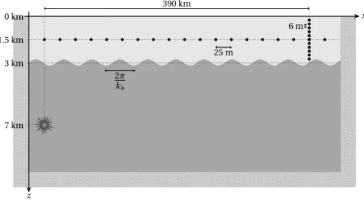
A domain 410 km long and 10 km thick provides a good compromise between model size and computation time (Fig. 1). It is vertically divided between a fluid ocean with a 3000 m mean depth and a solid crust 7 km thick. All sides, except the top sea-surface, are Perfectly Matched absorbing Layers (PML), which avoid unwanted reflections that would pollute the results [8]. The crust with the absorbing layer at

2π kh 25 m 6 m 7 km 390 km x z 0 km 3 km 1.5 km

Fig. 1. The calculation domain is made of a solid medium (dark grey) overlain by a fluid medium (light grey). The roughness of the sea-bottom is modelled by a sine function (18 m amplitude, 628 m wavelength; see text). The top side (sea–surface) is fully reflective, whereas the three other sides are Perfectly Matched absorbing Layers (hatched areas; 200 m thick). Black dots show the locations of the hydrophones where acoustic signals will be extracted. The source (star) is located 4 km under the rough bottom.

its bottom can thus be considered as a semi-infinite medium. The medium densities are set constant at typical values: 1000 kg.m−3 in the water and 3200 kg.m−3 in the crust, as the speeds of sound in the water (cw= 1500 m.s−1), and of

P-and S-waves in the crust (cP = 5000 m.s−1; cS = 3000 m.s−1,

resp.). This simple model does not consider a SOFAR channel (SOund Fixing And Ranging), which facilitates comparisons with analytical solutions. Moreover, the effects of refractions in the SOFAR is known to be negligible f or an ocean depth of 3km in the frequency band from 2.8 to 21.2 Hz [7]. The model also does not consider a sediment layer at the sea bottom, as its low shear-speed would require a mesh with very small finite elements that would considerably increase the calculation time. For the same reason, there is no attenuation either in the solid or in the fluid medium.

The roughness of the fluid/solid interface is modelled by a sine function; the water depth is thus defined by h(x):

h(x) = D + h0sin(khx), (1)

where D is the mean ocean depth (3000 m), h0= 18 m the

amplitude of the sinusoidal roughness and kh= 1.10−2 m−1

the bathymetry wavenumber, which corresponds to a wave-length 2π/kh' 628 m.

The source is located 4 km below the seafloor (i.e. 7 km below sea-surface). It is simulated by a Gaussian time-function with a central frequency at 10 Hz. The focal mechanism is an isotropic explosion, which simplifies the interpretation of the results where only PN-waves arrivals appear (no SN-waves). Its seismic moment (M0 = 4.03 × 1016 N.m) corresponds to

a medium magnitude earthquake (Mw= 5.0).

The calculation domain is meshed according to the speeds of propagation of the waves in both media, and the frequency content of the signal. Using SPECFEM2D internal mesher, we designed a mesh with 10,193 horizontal elements, 81 vertical elements in the crust and 93 in the ocean. The whole mesh is thus made of 1,773,582 elements, where the minimum number

of points per wavelength is 5.5 and the maximum frequency resolved is 27.4 Hz. The typical run-time is in the order of 7 hours on 86 parallel processors (3 cores), for a time signal of 600 s and a time-step of 5.10−4 s, which ensures the stability of the mesh for the considered element sizes and wave speeds. The time signal can be extracted anywhere in the mesh. The horizontal propagation of acoustic waves will be monitored with a horizontal antenna of hydrophones every 25 m at a 1500 m depth, along the whole calculation domain. The vertical structure of the wavefield, far enough from the source, will be examined with a vertical antenna of hydrophones every 6 m across the whole water column, located 390 km away from the source.

B. Modal propagation in numerical acoustic waves

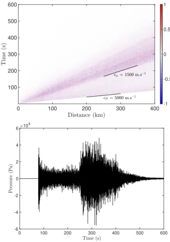
The different acoustic waves generated by the isotropic explosion can easily be sorted out in a distance-time diagram (Fig. 2-top), where the slope of the arrivals yields the speed of the waves. The first arrivals are PN-waves or acoustic waves propagating almost vertically in the water column but generated by P-waves propagating horizontally in the crust at 5000 m.s−1. The second and more energetic arrivals are T-waves or acoustic T-waves propagating in the water column at the sound speed (1500 m.s−1). The widening of the T-wave train suggests that these waves propagate as modes, with a modal dispersion increasing with the distance from the source. The time signal, 390 km away from the source and 1500 m below the sea surface (Fig. 2-bottom), shows typical features of abyssal T-waves: a low amplitude (comparable to the one of PN-waves) and an emergent wave-train [4]. The delay between PN-wave arrivals at 80 s and that of T-waves at 260 s is congruent with the distance from the source.

Using a 2D Fourier transform, the distance-time diagram (Fig. 2-top) can be converted in a frequency-wavenumber diagram (Fig. 3). The simulated dispersion curves can then be compared with the theoretical dispersion curves of Rayleigh modes in a finite-depth ocean overlaying on a semi-infinite elastic bottom [9]. The acoustic energy is located, between cw and cS, along Rayleigh modes and, for PN-waves, along

the line corresponding to cP. For a phase speed under cR =

2745 m.s−1, the theoretical speed of Rayleigh waves without an ocean, Rayleigh modes are acoustic waves propagating in the water column: T-waves. For a phase speed over cR,

Rayleigh modes are interface waves, evanescent in the crust but radiating energy in the water column. These interface waves arrive at a given hydrophone after the PN-waves and before the T-waves; they do not show on the distance-time diagram (Fig. 2-top), pr obably because they are hidden by PN-waves. PN-waves with a velocity higher than cP are generated

in the vicinity of the source, where P-waves in the crust cannot yet be considered to propagate horizontally. Zooming on Fig. 3 (bottom) shows Rayleigh modes still energetic up to frequencies congruent with observed T-waves (4-40 Hz, with a peak near ∼10 Hz). Moreover, the Rayleigh modes and PN-wave pattern is repeated in wavenumber, every kh, and

0 100 200 300 400 100 200 300 400 500 600 -1 -0.5 0 0.5 1 0 100 200 300 400 500 600 -6 -4 -2 0 2 4 6 10 4

Fig. 2. (Top) Distance-time diagram of the acoustic pressure normalized by its maximum at each hydrophone, in the case of an isotropic explosion below a rough bottom. (Bottom) Time signal 390 km away from the source and 1500 m below the sea surface, showing arrivals of PN-waves at 80 s and of T-waves at 260 s.

The frequency-wavenumber diagram clearly outlines the modal behavior of acoustic waves. However, to focus on the modal content of the signal and its spatial variation, we selected the sensor 390 km from the source and 1500 m below the sea surface and applied a non-linear warping function h(t) to the time t [10]: h(t) = s t2₊ r 2 c2 w , (2)

where r is the distance between the source and the sensor. The spectrum of a warped signal is turned into a frequency comb where each peak corresponds to a mode. As the peak corresponding to the nth mode, in a water layer with a depth D, is located at the frequency:

fcut=

cw(2n − 1)

4D , (3)

which is the cut-off frequency of the nth mode, the energy of each mode can be computed by applying a bandpass filter to the spectrum of the warped signal. In practice (Fig. 4-top), the spectrum of the warped signal is far more complex, due to the

0 10 20 30 40 50 60 70 80 0 5 10 15 20 25 0 1 2 3 4 5 6 7 8 0 0.5 1 1.5 2 2.5

Fig. 3. (Top) Frequency-wavenumber diagram of the normalized acoustic pressure showing the dispersion curves of simulated acoustic waves (col-ormap). Annotated black dashed lines show the phase speed of sound in water (cw), Rayleigh waves (cR), S-waves (cS) and P-waves (cP) and the

wavenumber of the sinusoidal topography (kh). (Bottom) Zoom of the

top-figure showing the theoretical Rayleigh modes (black dotted curves) matching the dispersion curves of simulated acoustic waves.

presence, in addition to the peaks at the cut-off frequencies of the modes, of their harmonics with frequencies multiplied by 2j

, j ∈ N. Unexplained peaks may be due to PN-waves. The variation of each mode-energy with depth, along a 3000 m vertical antenna 390 km far from the source, computed thanks to warping, follows the same variation as the energy of modes in a perfect waveguide (Fig. 4-bottom). Simulated and theoretical modes have the same number of nodes and anti-nodes, with a node at the sea surface and an anti-node at the sea bottom, which explains the possibility of conversion of seismic waves into acoustic waves at the sea bottom. The observed differences result from the fact that the warping function (2) is perfectly appropriate for modes in a perfect waveguide, i.e. modes in a finite depth ocean laying on a perfectly reflecting bottom, but not for Rayleigh modes.

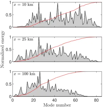
The comparison between the energies of the modes com-puted 1500 m below the sea surface at three locations — 10 km, 25 km and 100 km away from the source —shows that the long-distance propagation acts like a low-pass filter (Fig. 5). At 10 km from the source, modes are energetic up to

0 0.5 1 1.5 2 2.5 3 0 1000 2000 3000 4000 5000 6000 7000 0 0.5 1 0 500 1000 1500 2000 2500 3000 0 0.5 1 0 0.5 1 0 0.5 1

Fig. 4. (Top) Spectrum of a warped signal 390 km from the source and 1500 m below the sea surface showing the peaks corresponding to modes of T-waves (circles in red) and their second harmonic (circled in blue), fourth harmonic (circled in green), eighth harmonic (circled cyan) and sixteenth harmonic (circled in magenta). (Bottom) Comparison between the normalized energies versus depth of the 5th_{, 10}th_{, 15}th_{and 20}th_{modes computed from the spectra}

of warped signals from a vertical antenna 390 km from the source (blue) with the normalized energies versus depth of the same modes in a perfect waveguide (red). Energies are normalized by their maximum.

n = 85, whereas modes below n = 15 carry a negligible part of the total energy; at 25 km from the source, high modes remain energetic, but the relative energy of modes below n = 15 has grown; at 100 km from the source, the relative energy of modes below n = 15 is the same, but the energy of modes over n = 65 has almost vanished. The energy distribution remains almost unchanged at further distances (not shown here). The saw-tooth distribution of energy with modes, at the three distances, is an illustration that, at a given depth (here 1500 m), the energy of a given mode varies with the depth according to the node and anti-node distribution (Fig. ??-bottom).

The theory explaining Rayleigh modes also predicts the spectrum of PN-waves and its dependency on cw, cP, cS, the

densities of the fluid and solid media, and the water depth [9]. This theoretical spectrum has resonance peaks separated by about D/8cw and can be interpreted as the energy in the

frequency-wavenumber diagram along the line with a phase

0 0.5 1 0 0.5 1 0 20 40 60 80 0 0.5 1

Fig. 5. Normalized energy vs mode-number at 1500 m below the sea surface for three distances from the source: 10 km (top), 25 km (center) and 100 km (bottom). The energies are normalized by the energy of the most energetic mode. The red line show the cumulated energy normalized by its maximum.

speed cP (Fig. 3). In the same way, the theoretical spectrum

of SN-waves has peaks with the same periodicity, but at frequencies that differ from PN-waves, and that spectrum can be interpreted as the energy in the frequency-wavenumber diagram along the line with a phase speed cS. The spectrum of

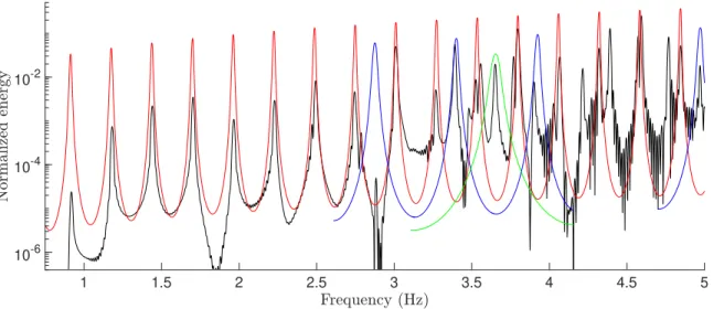
PN-waves 390 km away from the source and 1500 m below the sea surface is obtained from the first 140 s of the signal Fig. 2, hence avoiding the interface waves and T-waves arrivals. The normalized spectrum of simulated PN-waves is compared to the normalized theoretical spectrum (Fig. 6) and they both show a good agreement in the frequencies of the peaks and, in some cases, in the shape of the resonances. The simulated PN-wave spectrum also shows harmonics whose peak frequencies correspond to the frequencies of the theoretical peaks multi-plied by an integer. The number of harmonics is growing as the frequency grows and so the number of resonance peaks. The simulated spectrum does not show any SN-waves, since the focal mechanism is an isotropic explosion that generates only P-waves.

III. MODAL BEHAVIOR IN OBSERVED DATA

On December 4, 2015, at 22h24m54s GMT, a large mag-nitude (Mw = 7.1) intra-oceanic earthquake occurred in the

southern Indian Ocean at 47◦44.4’ S; 85◦ 10.98’ E, 16km below an abyssal plain, away from any shallow slope. Its signal was recorded by a vertical antenna made of two hydrophones, 987 km away from the epicenter, and located south of Amster-dam Island (42◦58.55’ S; 74◦31.41’ E; site SWAMS2; Fig. 7). The top hydrophone was 320 m below the sea surface and the

1 1.5 2 2.5 3 3.5 4 4.5 5 10-6

10-4 10-2

Fig. 6. Normalized spectra of simulated PN-waves (black) and of theoretical PN-waves (red) and their second (blue) and fourth (green) harmonics. Each spectrum is normalized by its maximum in the 1-10 Hz bandwidth.

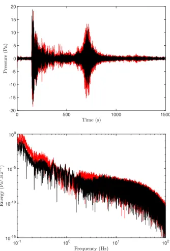
bottom hydrophone was in the axis of the SOFAR channel at a 1230 m depth. The recorded signals and their spectra are shown in Fig. 8. This signal has several common features with that simulated in Fig. 2-top : the predicted PN-waves and T-waves have the same relative amplitudes, shapes and delays as observed, despite all the simplistic assumptions of the model.

−4500 −4000 −3500 −3000 −2500 −2000 −1500 2 Amsterdam Kerguelen SWAMS2

65˚E 70˚E 75˚E 80˚E 85˚E

50˚S 45˚S 40˚S 35˚S meters Mw=7.1

Fig. 7. Bathymetric map in the Southern Indian Ocean showing the locations of the December 04, 2015 magnitude Mw=7.1 earthquake and of the

SWAMS2 hydrophone antenna where it was recorded (Fig. 8).

The comparison between the spectra from the two

hy-drophones at different depths gives a clue on the possible modal propagation of observed abyssal T-waves. The spectrum of the data from the deepest hydrophone (red in Fig. 8-bottom) shows that surface waves are dominant below 0.5 Hz, PN- and SN-waves are dominant between 0.5 and 1 Hz and T-waves are dominant above 1 Hz. We observe the same waves on the spectrum from the uppermost hydrophone, except that the T-wave energy is lower between 1 and 4 Hz. Until 3 Hz, the slope of the spectrum from the uppermost deep hydrophone is the same as in the frequency band dominated by PN- and SN-waves and over 3 Hz, energy rises until it reaches the value of the lowest hydrophone at 4 Hz. This energy gap in the T-waves spectrum recorded by the uppermost hydrophone can be explained by the theory of normal modes. Every mode shows a node at the sea surface where their energy is minimal. Low-order modes have fewer nodes and the first anti-node below the sea surface, where their energy is maximal, is localized deeper than with higher modes. Hence, near the sea surface, the energy of low-order modes, which are dominant for low frequencies, is very low and this is consistent with the energy gap we observe between the top and bottom hydrophones.

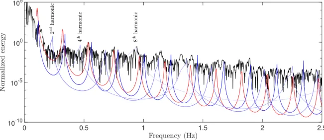
A focus on the spectrum of PN- and SN-waves brings stronger evidence of a modal behavior. The spectrum of the first 500 s of the signal from the uppermost hydrophone shows both PN- and SN-waves. This spectrum can be compared to the theoretical spectra of PN- and SN-waves in the same way as in section II-B and Fig. 6. Theoretical spectra are computed for the water-depth at the hydrophone antenna (3500 m), with a mean speed of sound of 1480 m.s−1 and a speed of the PN-waves (8100 m.s−1) and SN-waves (4700 m.s−1) in the upper mantle, assuming the observed PN- and SN-waves were refracted in the mantle. Preliminary computations (not shown here) show that the frequencies of energy peaks, which is here the most pertinent parameter for comparing theory and

0 500 1000 1500 -20 -15 -10 -5 0 5 10 15 20 10-1 100 101 102 10-15 10-10 10-5 100

Fig. 8. (Top) Hydroacoustic data, high-pass filtered at 0.5 Hz to remove surface waves, of the December 4, 2015 earthquake, recorded 987 km away by hydrophones at 320 m (black) and 1230 m (red) below the sea surface. (Bottom) Spectra of the two unfiltered time-signals.

data, are insensitive to the choice of the medium densities. We chose 1000 kg.m−3 as the density of sea water and 3200 kg.m−3 as the density of the oceanic crust, typical of oceanic basalts. The comparison between the spectrum from the data and the theoretical spectra normalized by their energy at 0.1Hz (Fig. 9) shows a good agreement in the frequencies of the energy peaks. The spectrum also shows harmonics of SN-waves whose peak frequencies correspond to that of the theoretical peaks multiplied by an integer. For matching purpose, we normalized the second and the fourth harmonic to adjust their second visible peak on a peak from the data and we did the same for the only visible peak of the eighth harmonic.

IV. CONCLUSION

The 2D finite element modeling applied to a simple configu-ration with a sinusoidal roughness on the sea bottom correctly reproduces the generation of PN-waves and abyssal T-waves. The synthetic signals display the same features as observed signals in terms of the wave envelope and arrival times. The synthetic T-waves propagate as modes whose dispersion matches an analytical solution; their vertical structure and

changes of the acoustic modes over long-range propagation are similar to the ones expected by theory. The spectrum of PN-waves also follows an analytical solution, with the addition of the presence of harmonics. Observed abyssal T-waves, generated by an intra-oceanic earthquake and recorded by an antenna of two hydrophones at different depths, present a vertical structure that can be interpreted in terms of modes. The spectrum of PN- and SN-waves in the observed signal matches fairly well the analytical solution used to predict the spectrum of synthetic PN-waves.

ACKNOWLEDGEMENTS

J. Lecoulant is supported by a joint PhD grant from the D´el´egation G´en´erale de l’Armement (DGA) and the University of Brest (UBO). The SPECFEM3D code was run on Datarmor, a massive computing facility common to several research institutions at the westernmost tip of Brittany (France).

REFERENCES

[1] Tolstoy, L. and Ewing, W.M., “The T-phase of shallow-focus earth-quakes,” Bull. Seismol. Soc. Amer., vol. 40, p. 25–52, 1950.

[2] de Groot-Hedlin, C.D. and Orcutt J.A., “Excitation of T-phases by seafloor scattering,” J. Acoust. Soc. Am., vol. 109(5), p. 1944-1954, 2001.

[3] Fox, C.G., Dziak, R.P., Matsumoto, H., Schreiner, A.E., “Potential for monitoring low-level seismicity on the Juan de Fuca Ridge using military hydrophone arrays,” Mar. Tech. Soc. J., vol. 27(4), p. 22–30, 1994. [4] Okal, E. A., “The generation of T waves by earthquakes,” Advances in

Geophysics, vol. 49, p. 1–65, Elsevier, 2008.

[5] Tromp, J., Komatitsch, D., and Qinya, L., “Spectral-element and adjoint methods in seismology,” Communications in Computational Physics, vol. 3(1), p. 1–32, 2008.

[6] Cristini, P. and Komatitsch, D., “Some illustrative examples of the use of a spectral-element method in ocean acoustics,” J. Acoust. Soc. Am., vol. 131(3), EL229-EL235, 2012.

[7] Jamet, G., Guennou, C., Guillon, L., Mazoyer, C., and Royer, J.-Y., “T-wave generation and propagation: A comparison between data and spectral element modeling,” J. Acoust. Soc. Am., vol. 134(4), p. 3376– 3385, 2013.

[8] Xie, Z., R. Matzen, P. Cristini, D. Komatitsch, and R. Martin, “A perfectly matched layer for fluid-solid problems: Application to ocean-acoustics simulations with solid ocean bottoms,” J. Acoust. Soc. Am., vol. 140(1), p. 165–175, 2016.

[9] Ardhuin, F. and Herbers, T. H. C., “Noise generation in the solid Earth, oceans and atmosphere, from nonlinear interacting surface gravity waves in finite depth,” J. Fluid Mech., vol. 716, p. 316–348, 2013.

[10] Bonnel, J., Nicolas, B., and Mars, J.I. “Estimation of modal group velocities with a single receiver for geoacoustic inversion in shallow water,” J. Acoust. Soc. Am., vol. 128 (2), p. 719–720, 2010.

0 0.5 1 1.5 2 2.5 10-10

10-5 100 105

Fig. 9. Normalized spectrum of observed PN- and SN-waves (black), normalized spectrum of theoretical PN-waves (red), normalized spectra of 1st_{, 2}nd_{, 4}th