HAL Id: ird-01905147
https://hal.ird.fr/ird-01905147
Submitted on 25 Oct 2018
HAL is a multi-disciplinary open access archive for the deposit and dissemination of sci-entific research documents, whether they are pub-lished or not. The documents may come from teaching and research institutions in France or abroad, or from public or private research centers.
L’archive ouverte pluridisciplinaire HAL, est destinée au dépôt et à la diffusion de documents scientifiques de niveau recherche, publiés ou non, émanant des établissements d’enseignement et de recherche français ou étrangers, des laboratoires publics ou privés.
Nicola Dal Ferro, F Morari
To cite this version:
Nicola Dal Ferro, F Morari. From real soils to 3D-printed soils : reproduction of complex pore network at the real size in a silty-loam soil. Soil Science Society of America, 2015. �ird-01905147�
For Review Only
From real soils to 3D-printed soils: reproduction of complex pore network at the real size in a silty-loam soil
Journal: Soil Science Society of America Journal Manuscript ID: S-2015-03-0097-OR.R2
Manuscript Type: Papers on Original Research
Keywords: X-ray computed microtomography , soil structure, 3D print, saturated hydraulic conductivity
For Review Only
1
From real soils to 3D-printed soils: reproduction of complex pore network at the real size in a 1
silty-loam soil 2
3
N. Dal Ferroa, F. Moraria* 4
a
Department of Agronomy, Food, Natural resources, Animals and Environment, Agripolis,
5
University of Padova, Viale Dell’Università 16, 35020 Legnaro (Padova), Italy
6
7
Abstract 8
Pore complexity and micro-heterogeneity are pivotal in characterizing biogeochemical processes in 9
soils. Recent advances in X-ray computed microtomography (microCT) allow the 3D soil 10
morphology characterization of undisturbed samples, although its geometrical reproduction at very 11
small spatial scales is still challenging. Here, by combining X-ray microCT with 3D multijet 12
printing technology, we aimed to evaluate the reproducibility of 3D-printing soil structures at the 13
original scale with a resolution of 80 µm and compare the hydraulic properties of original soil 14
samples with those obtained from the soil-like prototypes. Results showed that soil-like prototypes 15
were similar to the original samples in terms of total porosity and pore shape. By contrast the pore 16
connectivity was reduced by the incomplete wax removal from pore cavities after the 3D printing 17
procedure. Encouraging results were also obtained in terms of hydraulic conductivity since 18
measurements were successfully conducted on five out of six samples, showing positive correlation 19
with experimental data. We are confident that future developments of 3D-printing technologies and 20
of their combination with microCT will help to further the understanding of soil micro-21
heterogeneity and its effects on soil-water dynamics. 22
For Review Only
1. INTRODUCTION24
The processes that form porous media lead to highly heterogeneous three-dimensional structures, 25
forcing scientists to adopt models for reproducing the reality. This is the case for soil physics, which 26
has its foundations laid on the capillary bundle model (Hunt et al., 2013). Water flow is still 27
commonly conceptualized as a 2D bundle of cylindrical tubes passing through the soil only in the 28
vertical direction, trivializing the natural complexity of a soil. As a result, derived models such as 29
those of water conductivity (Burdine, 1953; Mualem, 1976) introduced empirical adjustments (e.g. 30
a tortuosity factor) to compensate for fundamental errors in the conceptual model (Hunt et al., 31
2013). The simplification of reality in one-dimensional or two-dimensional models was supported 32
by the inability to see and understand the 3D structure and its interactions with biota due to its 33
opaque nature (Feeney et al., 2006). However, recent advanced technologies have provided a vast 34
amount of data and their assimilation in more complex models that have partly superseded the use 35
of reduction methods (Ahuja et al., 2006). The first steps for creating real-world situations in soil 36
science used 3D random network models (e.g., Rajaram et al., 1997; Peat et al., 2000) that 37
mimicked the soil complexity and dynamics in a three-dimensional space. In spite of their overall 38
improvement in the understanding of matrix flow and transport of solutes, these models had two 39
main limitations: a) computing limitations make some structural simplification unavoidable and b) 40
the soil has such structural complexity that a reliable estimate of a representative elementary 41
volume is difficult to quantify (Peat et al., 2000), as for most of the models. Lately, non-invasive 42
imaging approaches have gained attention as they provide the opportunity to examine soil-water 43
interactions from direct observations at the microscale. For example, the soil physical and chemical 44
processes were replicated using high-tech materials with a refractive index similar to water, 45
allowing the use of 3D optical microscopy in a transparent-reconstructed medium for the 46
visualization of biophysical processes. Controlled experiments of how pore channels can influence 47
For Review Only
3
the biological and hydraulic dynamics can be realized, although the reconstructed medium is only 48
partially reproducible because it is composed of single incoherent particles (Downie et al., 2012). 49
Impressive developments and insights into porous media research have also been provided by X-ray 50
computed microtomography (microCT) that allows microscopic visualization of the spatial 51
arrangement of complex structures (Cnudde and Boone, 2013). For the first time it became possible 52
to investigate the interior of an object in a non-destructive way and to extract qualitative and 53
quantitative information of multiphase porous materials (e.g., Tippkoetter et al., 2009; Mooney et 54
al., 2012). In this context “digital rock physics”, i.e. the study of pore scale processes by the use of 55
digital imaging and modelling, has expanded enormously the understanding of single and 56
multiphase flow dynamics (Blunt et al., 2013). 57
Only recently 3D-printers have gained attention in the design of niche products, prototypes and one-58
time creations (e.g., Rangel et al., 2013), although the technology is 30-years old. This technology 59
has been proposed in research as a tool to integrate virtual microCT information with real building 60
models. In fact, the combination of such techniques make it possible to reconstruct complex 61
microcosms with the heterogeneity discovered with microCT at a resolution of few micrometers, 62
providing the opportunity to isolate the physical and chemical aspects that govern the 63
biogeochemical and microbial processes in the soil (Otten et al., 2012; Ju et al., 2014; Bacher et al., 64
2015; Ringeisen et al., 2015). Nowadays, with 3D printing the diversified geometry encountered in 65
a soil can be replicated at a resolution of tends of micrometers. Several materials can be used 66
including plastics, resins, ceramics and metals. 67
Despite large uncertainties persisting about soil microscale heterogeneity and its effects on the 68
macroscopic dynamics (Baveye et al., 2011), so far few have tried to combine high-resolution 3D 69
imaging and printing technology to improve knowledge in soil science. In this study we combined 70
3D printing technology with X-ray microCT in an attempt to reconstruct the 3D complexity of the 71
For Review Only
soil structure in a soil-derived model at the same spatial scale as the original one and test some 72
hydraulic properties. 73
74
2. MATERIAL AND METHODS 75
Experimental design and soil sampling
76
The soil samples come from a long-term experiment established in 1962 at the experimental farm of 77
the University of Padova (Italy). The soil (Table 1) is Fluvi-Calcaric Cambisol (CMcf), silty loam 78
(FAO-UNESCO, 1990). This work considered soil samples from a long-term trial that compares 79
two treatments: farmyard manure at 60 t ha−1 y−1 (hereafter labelled “M”) and a no fertilization 80
control (hereafter labelled “C”) on a continuous maize crop system. The same type of tillage has 81
been used for both treatments, with autumn plowing and subsequent cultivations prior to sowing the 82
main crop. The experimental layout is a randomized block with three replicates, on plots of 7.8 × 6 83
m. Further details on experimental design are extensively reported in the literature (e.g., Morari et 84
al., 2006). A total of six undisturbed soil cores (5 cm diameter, 6 cm length) were collected in 85
August 2010 (Fig. 1, step A), at the end of the maize season, from the topsoil (5 to 20 cm depth) in 86
polymethylmethacrylate (PMMA) cylinders using a manual hydraulic core sampler (Eijkelkamp, 87
The Netherlands). Cores were stored at 5 °C until analysis. 88
89
MicroCT soil scanning and image processing
90
The pore structure of soil cores, labelled “Msoil” and “Csoil” for farmyard manure and no
91
fertilization control, respectively (Fig. 1, step B) was sampled using X-ray computed 92
microtomography (microCT). In order to allow the scanning of the whole soil core at a fine 93
resolution, samples were analyzed at the “3S-R” facility in Grenoble (http://www.3sr-grenoble.fr//) 94
For Review Only
5
at a spatial resolution of 40 µm. Setting parameters were 100 kV, 300 µA and projections were 95
collected during a 360° sample rotation at 0.3° angular incremental step. Each projection was the 96
mean of 10 acquisitions and scan frequency was 7 images s-1. Beam hardening artifacts were 97
minimized during data acquisition using a 0.5 mm Al filter. In order to avoid pixel misclassification 98
that might occur during projection measurements due to scattered radiation, nonlinearity of data 99
acquisition systems, partial volume effects etc. (Hsieh, 2009), 2D projections were resized after 100
acquisition using a mean filter by a two-pixel factor along the vertical and horizontal axis. As a 101
result, the reconstructed images had a coarser resolution than that of acquisition (i.e. 80 µm). 102
Resized projections were finally reconstructed using the dedicated software DigiCT 1.1 (Digisens, 103
France) to obtain a stack of about 750 2D slices in 32-bit depth. 32-bit images were later converted 104
into 8-bit depth. 105
The digital image processing and analysis of soil samples, conducted with the public domain image 106
processing ImageJ (Vs. 1.45, National Institute of Health, http://rsb.info.nih.gov/ij), has already 107
been reported in (Dal Ferro et al., 2013). Briefly, a cylindrical volume of interest with a diameter of 108
600 pixels and composed of 600 slices (4.8 cm height × 4.8 cm diameter) was selected in order to 109
exclude the PMMA sample holder. Slices were segmented using a global-threshold value based on 110
the histogram greyscale that was determined by the maximum entropy threshold algorithm. The 111
threshold value was selected where the inter-class entropy was maximized (Luo et al., 2010). 8-112
connectivity, a mathematical morphology closing operator (Serra, 1982), was applied to the binary 113
images to fill misclassified pixels inside the pores as well as to maintain pore connections (Mooney 114
et al., 2006). Successively, the one interconnected pore network (infinite cluster) that contained 115
most of the porosity within each stack was extracted and analyzed with CTAn software v. 1.12.0.0 116
(Bruker micro-CT, Kontich, Belgium) as this pore space was the only one to show continuity 117
between the top and bottom of the soil cores. Although more connections between pores were likely 118
present within the soil cores, microCT imaging provided only connections larger than the resolution 119
For Review Only
limits, restricting our analysis to the soil macroporosity. A description of the soil morphological 120
parameters as a result of microCT scanning has already been reported in Dal Ferro et al. (2015) 121 (Table 1). 122 123 3D mesh generation 124
A surface mesh model for each sample (3 replicates × 2 treatments) was extracted from the one 125
interconnected pore network that was identified from the microCT stacks using the free software 126
InVesalius 3.0 (CTI, Campinas, São Paulo, Brazil) (Fig. 1, step G). The created model was then 127
exported in the geometrical stereolithography file format encoded in Standard Tessellation 128
Language (STL). The reconstructed STL model, composed of 10 to 30 million triangles depending 129
on the complexity of the pore network, was visualized with the open-source software MeshLab 130
v.1.3.2 (STI-CNR, Rome, Italy; http://meshlab.sourceforge.net/) in order to assess the continuity of 131
pore connections along the vertical axis and successively simplified to a polygonal mesh that 132
consisted of up to 10 million triangles. In order to compare the microCT imaging from the original 133
samples with the 3D-printed prototypes from the STL model, one of the three replicate microCT 134
stacks was selected for both “M” and “C”. Afterwards a volume of interest, corresponding to a 135
cylinder of 300 pixels height × 300 pixels of diameter (Fig. 1, step C), was extracted by both 136
samples (2.4 cm high × 2.4 cm diameter). InVesalius 3.0 was used to obtain a polygonal mesh 137
model, from which a STL file was exported (Fig. 1, step D). MeshLab v.1.3.2 was used to simplify 138
the polygonal mesh at two levels of detail, corresponding to 500 thousand (500k) and 10 million 139
(10M) triangles respectively. Each model was 3D-printed twice (Fig. 1, step E), resulting in a total 140
of eight models (2 soil samples × 2 generated meshes × 2 replicate printings). All the closed pores, 141
i.e. the pores that had no connection to the space outside, were then digitally removed from the 142
stacks since they cannot contribute to flow properties of the model. 143
For Review Only
7
3D printing
145
Lastly, 14 polygonal meshes (6 cylinders, 4.8 cm h × 4.8 cm diameter; 8 cylindrical subsamples, 2.4 146
cm h × 2.4 cm diameter) were built with a commercial 3D printer. The printer (ProJet 3510 HD, 3D 147
Systems, http://www.3dsystems.com/) was selected as it provided a fast prototype reconstruction 148
with high resolution and available at a relatively low price (few hundred €). The 3D structure was 149
printed with resin whose exact composition is proprietary but approximately contained an organic 150
mixture of: ethoxylated bisphenol A diacrylate (15-35%), urethane acrylate oligomers (20-40 %), 151
tripropyleneglycol diacrylate (1.5-3%) (Visijet Crystal, EX 200 Plastic material, Safety Data Sheet, 152
http://www.3dsystems.com). The 3D printer has a multijet printing technology, i.e. an inkjet 153
printing process that deposits either photocurable plastic resin or casting wax materials layer by 154
layer, with a spatial resolution of 29 µm and a declared accuracy of 25-50 µm, depending on 155
building parameters and prototype size and geometry. The final result was a set of solid prototypes 156
whose pores were filled with paraffin wax (the contact angle between water and wax, measured 157
with a goniometer, was 120°), while the soil matrix was composed of the resin. The contact angle 158
between the pure resin (cleaned of any wax) and the water, measured with a contact angle 159
goniometer, was 69°. 160
161
Wax removal procedure
162
Wax removal is crucial in order to empty the pores and accurately replicate the complex geometry 163
of the soil samples. Ultrasonication in oil at a temperature of 60 °C and 60 Hz for 24 h and oven 164
drying at 60 °C until stabilized weight (ca. four days) were adopted as possible procedures to empty 165
the pores. Alternative methods were considered: the use of xylene or vapor steam cleaning would 166
have dissolved the wax, although it would have probably corrupted the solid pore surface, while 167
alternative printing technologies without the use of wax as a physical support during 3d printing 168
For Review Only
were not feasible. As a result, we adopted a simple and relatively low-cost combination between 3D 169
printing technology and cleaning procedure. 170
171
3D prototypes scanning, image reconstruction and analysis
172
The resulting prototypes from the sub-volume of the samples (i.e. “Msmall” and “Csmall” at a detail of
173
500 thousand and 10 million triangles) were finally subjected to X-ray microCT scanning (Fig. 1, 174
step F) in order to assess: a) the reproducibility and reliability of the 3D printing process; b) the 175
smoothing effect of polygon reduction on the generated 3D structure; c) efficacy of the cleaning 176
procedure to remove the wax from the pores. Prototypes were analyzed with a Skyscan 1172 X-ray 177
microtomography (Bruker micro-CT, Kontich, Belgium) at the University of Padova since lower 178
energy than those used for scanning the whole soil sample was required to penetrate the specimen. 179
Setting parameters were 40 kV, 250 µA and projections were collected during a 180° sample 180
rotation at 0.25° angular incremental step. Each projection was the mean of eight acquisitions and 181
scan frequency was 1.33 images s-1. Beam hardening artifacts were minimized during data 182
acquisition using a 0.5 mm Al filter. The spatial resolution was 27 µm. In order to avoid pixel 183
misclassification that might occur during image acquisition (Hsieh, 2009), projections were resized 184
after acquisition using a mean filter by a two-pixel factor along the vertical and horizontal axis. As a 185
result, the reconstructed images had a final resolution twice that of acquisition (i.e. 54 µm). Resized 186
projections were reconstructed using the dedicated software NRecon v. 1.6.9.4 provided by Bruker 187
micro-CT to obtain a stack of about 450 2D slices in 16-bit depth. 16-bit images were later 188
converted into 8-bit depth. 189
Prototype matrix, wax and void phases were easily visualized and binarized with a single threshold 190
level. 8-connectivity was applied to the binary images to fill misclassified pixels inside the pores as 191
well as to maintain pore connections (Mooney et al., 2006). MicroCT porosity (m3 m-3), pore size 192
For Review Only
9
distribution and open porosity (%), pore surface to volume ratio (µm-1), 3D fractal dimension and 193
Euler number (mm-3) were estimated from each binarized stack using CTAn and compared with soil 194
parameters obtained from the original sub-volume samples. 195
196
Hydraulic conductivity test on 3D-printed prototypes
197
Saturated hydraulic conductivity (Ks-large) measurements were conducted on the large prototypes
198
(“Mlarge” and “Clarge”, 4.8 cm high × 4.8 cm diameter) (Fig. 1, step H) by using a laboratory
199
permeameter (Eijkelkamp, The Netherlands) that was adjusted to the size of the samples by using a 200
gasket whose thickness created a seal at the interface between the prototype and the sample holder. 201
Ks-large was determined with both constant and variable head method, according to the hydraulic
202
properties of the medium. As a rule of thumb, Ks-large values greater than 5.8 10-6 m s-1 were easily
203
determined by the constant head method, while the falling head method was conducted at smaller 204
Ks-large values. Before conducting the analysis and to ensure that water flowed only vertically from
205
the top to the bottom of the prototypes, avoiding the loss of water from lateral pores, samples were 206
firstly sealed with a plastic tape and successively coated with a layer of melted wax. As a result, it 207
was ensured the complete sealing of the samples avoiding the lateral occlusion of interior pores. 208
Successively samples were freely upward saturated at atmospheric pressure (water bath reached ¾ 209
of sample height) using de-aerated water, then subjected to 0.6 10-5 Pa to completely de-aerate them 210
and saturated again as above. 211
212
Hydraulic conductivity test on original samples
213
Saturated water conductivity on soil-like prototypes was compared with water flow calculated on 214
the original soil samples and already proposed in (Dal Ferro et al., 2015). As a result, original 215
samples were subjected to saturated water conductivity analyses (Ks-soil, m s-1) using the constant
For Review Only
head or falling head method, depending on the soil properties and range of Ks-soil that can be
217
measured (Reynolds et al., 2002). In addition, the microCT imaging dataset of the original samples 218
(scanned at the “3S-R” facility in Grenoble) was used to calculate water conductivity on the one 219
interconnected pore cluster (KMorph, m s-1) by using a morphologic approach as proposed by (Elliot
220
et al., 2010). Briefly, the model consisted of combining three dimensional pore shape parameters 221
with pore volume and using a modified Poiseuille equation as follows: 222 ν π c L P R Q 8 4∆ = , [1] 223
where R is pore radius, ν is the viscosity of water at room temperature, ∆P is the change in 224
hydrostatic pressure and Lc is the pore length, depending on pore shape characteristics.
225
Lastly, rearrangement of Darcy’s law allowed the KMorph estimation for the extracted pore network:
226 P A QL K ∆ = , [2] 227
where A is the cross-sectional area of the sample and L is the sample length. A detailed description 228
of the methods and results for the soils proposed here can be found in Dal Ferro et al. (2015). 229
230
3. RESULTS 231
Soil volume and prototype measurements
232
Ultrasonication in oil was only partially able to remove the wax from pores, while the subsequent 233
oven drying at 60 °C was able to remove most of it (Fig. 2). A further increase in temperature was 234
not possible because, according to the manufacturer, it would have weakened the resin structure or 235
melted part of it. As a result, the combination of both techniques was used as the best procedure 236
currently available to successfully empty the open pores as well as maintain the solid structure. 237
For Review Only
11
However, the continuing advances in 3D-printing technology and the use of heat-resistant materials 238
will allow the full removal of the support material (e.g. by evaporation). 239
Soil porosity of sub-volumes scanned with microCT (“Msoil” and “Csoil” 2.4 cm high × 2.4 cm
240
diameter) was entirely connected to the space outside the soil matrix (open pores/total porosity = 241
100%), but highly different between “Msoil” (0.114) and “Csoil” (0.036) (Table 2). The open pores of
242
“Msmall” prototypes were slightly lower than porosity detected by microCT, with negligible changes
243
between 500 thousand (500k) and 10 million (10M) triangle meshes. Indeed, only 2.4% of microCT 244
porosity (0.109 and 0.110 in 500k and 10M, respectively) was confined within the solid phase 245
(Table 2). By contrast, the “Csmall” prototypes showed a consistent increase of confined pores with
246
respect to the total ones, ranging from 15.1% in the 500k to 18.4% in the 10M meshes, on average. 247
As a result, the “Csoil” porosity (0.036) was slightly greater than “Csmall” built both from 500
248
thousand (0.024) and 10 million (0.027) triangle meshes respectively. 249
Pore size distribution (PSD) curves (Fig. 4), measured on microCT images in volumetric terms 250
according to the medial-axes determination and sphere-fitting measurement (Remy and Thiel, 251
2002), were distributed differently between “M” and “C”. In “M” the most frequent pore classes 252
were distributed between 240 µm and 560 µm diameter, while they were shifted towards smaller 253
pores in “C”, ranging between 160 µm and 440 µm. Comparable data were found between PSD 254
prototype classes, in both “M” and “C”, with negligible variations between replicates and meshes. 255
By contrast, a sharp increase of the small pores was observed in the original samples with respect to 256
the prototypes: this was particularly clear for pore classes smaller than 800 µm and 490 µm in 257
“Msoil” and “Csoil”, where the integral of the PSD differences was around 30% and 10% of microCT
258
porosity, respectively. Finally, it was noticed that some pores were still filled with wax despite its 259
melting and removal with ultrasonication and oven drying (Fig. 3). In particular, wax most resided 260
in thin throats (< 200 µm, on average) between largest cavities, leading to their disconnection and 261
thus increasing both the average size of empty pores and the number of isolated ones. 262
For Review Only
Pore morphological features (Table 2), estimated by means of pore surface/volume ratio (µm-1), 263
Euler number (i.e. an indicator of pore connectivity, where the greater is the value, the lower is the 264
pore connectivity; mm-3) (Vogel et al., 2010) and 3D fractal dimension (box-counting method) 265
(Perret et al., 2003), emphasized the self-similarity between the prototypes that were generated by 266
the same original sub-volume. For instance, the pore surface/volume ratio was 0.007 µm-1 in 267
“Msmall” prototypes as characterized by different meshes (500k and 10M triangles), while the fractal
268
dimension (2.42 and 2.25 in the original “Msoil” and “Csoil”, respectively) ranged in “Msmall”
269
between 2.10 (500k triangles) and 2.62 (10M triangles) and in “Csmall” between 2.38 (500k
270
triangles) and 2.55 (10M triangles). Only the Euler number parameter, particularly in “Msmall” and
271
“Csmall” built from 500k triangle meshes, showed high variability between the prototypes (Table 2).
272
273
Experimental saturated hydraulic conductivity measurements on large prototypes
274
Experimental saturated hydraulic conductivity (Ks-large) data were obtained on five of the six
275
reconstructed large prototypes (“Mlarge” and “Clarge” 4.8 cm high × 4.8 cm diameter, an example is
276
reported in Fig. 5) since water did not flow through one of the “Clarge” samples (Table 3). Ks-large
277
was generally higher in “M” (18.5 m s-1, on average) than “C” (0.035 m s-1, on average), ranging 278
between a minimum of 0.023 m s-1 observed in “C” and a maximum of 13.5 m s-1 in “M. The water 279
flow measurements on the prototypes were generally greater (7.65 10-5 m s-1, on average) than those 280
measured (Ks-soil = 3.59 10-6, on average) and modelled (KMorph = 1.91 10-6 m s-1) on the original soil
281
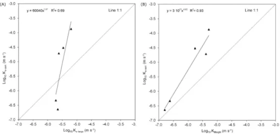
samples (Table 3) (Dal Ferro et al., 2015). Finally, positive correlations were observed between 282
soil-like Ks-large values and both Ks-soil (R2 = 0.69) and KMorph (R2 = 0.93, Fig. 6).
283
284
4. DISCUSSION 285
For Review Only
13
The comparison between morphological characteristics of replicated small prototypes (“Msmall” and
286
“Csmall”) showed that 3D printing technology was able to retain the basic features of the macropore
287
network. More specifically, the pore size and shape characteristics of the largest pores was easily 288
visualized on the microCT imaging (Fig. 3), highlighting the similarity between reconstructed 289
models. Moreover, introducing some smoothing of the surface walls by the simplification of the 290
mesh (500 thousand vs. 10 million triangles) did not show significant changes between macropore 291
characteristics. In particular, the “M” microCT porosity and pore surface/volume ratio had a 292
coefficient of variation of 3.6% and 4.8%, respectively. These results were supported by others: 293
Otten et al. (2012) reported a very high reproducibility of twelve prototypes since the measured 294
porosity (0.66) was characterized by a very low coefficient of variation (3.36%), although their soil-295
like prototypes were scaled up three times with respect to the original size of the soil samples. By 296
contrast, our prototypes were reconstructed at the real size, although the soil microscale 297
heterogeneity that was provided by the fine silt and clay particles could not be faithfully reproduced 298
due to the microCT soil scanning (40 µm) and 3D printing resolution limits (29 µm). 299
The successful reproduction of generated “Msmall” prototypes (Fig. 1, step E) was partly reappraised
300
by evaluating the pore morphological characteristics in detail (Table 2). In fact, the pore structure 301
parameters varied between the reconstructed models, especially in the “Csmall” prototypes. For
302
instance, the coefficient of variation of total porosity was 11.5% in the “Csmall” prototypes,
303
increasing to 63% in the Euler number. Nevertheless, it is worth noticing that the microCT scanning 304
of small prototypes (Fig. 1, step F) was performed at a resolution (27 µm) that was finer than that 305
used during the 3D-printing (29 µm, ± 50 µm), emphasizing the systematic errors during the model 306
building process. As a result, the mismatch observed between soil samples (“Msoil” and “Csoil”) and
307
prototypes (“Msmall” and “Csmall”) structures were the result of the combined effect between: a) soil
308
digital imaging due to microCT scanning; b) inaccuracy during the 3D printing process; c) 309
prototype digital imaging due to microCT scanning. Furthermore, the 3D mesh generation created 310
For Review Only
distorted elements from the voxel-based microCT volumes, although the negligible variations 311
between small prototypes as printed from 500 thousand and 10 million triangles suggested their 312
minor role during the prototypes production. Moreover, the partial effectiveness of wax removal 313
from the macropores (Fig. 3), quantified at around 2.4% (“Msmall”) and 16.7% (“Csmall”) of microCT
314
porosity, increased the uncertainty on the pore quantity and morphology. Finally, the biggest 315
differences were observed in terms of Euler number, showing its ability to identify slight structure 316
changes between replicated prototypes. The wax entrapped in the voids created a discontinuity 317
between adjacent pores by modifying the degree of connection of the macropore network and partly 318
isolating them from the space outside the solid matrix. As a result, the soil volumes (“Msoil” and
319
“Csoil”) generally had both a higher microCT total porosity and a lower Euler number (i.e. more
320
connections) than the reconstructed prototypes (Table 2). As suggested by the pore size distribution 321
analysis, the wax was easily removed from the largest pores, while it consistently remained in the 322
smallest ones (Fig. 4). Finally, a mismatch between soil and soil-like porosity was probably 323
introduced during microCT soil analysis and the following mesh generation. Indeed microCT 324
imaging was composed of cubic voxels while polygonal mesh comprised a surface triangulation, 325
avoiding their full overlap. 326
In spite of the difficulty in totally cleaning the wax from the macropores, measurements of saturated 327
hydraulic conductivity were successfully conducted on five of the six large prototypes. Only the 328
saturated conductivity measurement on one “Clarge” prototype failed. Since one of the “Clarge”
soil-329
derived model was characterized by the lowest total porosity (0.015), most likely the entrapped wax 330
occluded the scarce conductive pores within the whole prototype and prevented flow. Water flow 331
measurements, calculated through the one interconnected macropore network that spanned the 332
sample, were highly correlated with properties calculated on the original samples (Ks-soil) and
333
particularly with those modelled (KMorph) on the same pore network (Fig. 6) (Dal Ferro et al., 2015).
334
Nevertheless, Ks-large had higher values than Ks-soil and KMorph by at least one order of magnitude in
For Review Only
15
the “M” treatment (Table 3), although the total porosity had been reduced with respect to the soil 336
sample ones in two ways: a) the prototypes were reconstructed on the basis of digital imaging from 337
microCT scanning that performed at a resolution that excluded all the small connections between 338
the largest pores and decreased the adsorption along the macropore walls; b) part of microCT 339
porosity was probably still filled with wax during Ks-large measurements, reducing the water flow
340
capacity of the porous medium. These results suggested the major role of conducting macropores on 341
water flow dynamics (Jarvis, 2007), although the undetected and unprinted micropores < 80 µm 342
might have partially increased Ks-large to approach the experimental Ks-soil (Elliot et al., 2010),
343
particularly when the soil structure was largely composed of thin pores and microcracks are often 344
insufficiently imaged with microCT and thus underrepresented (i.e. in the control samples), 345
especially in the vicinity of grain contacts (Andrä et al., 2013). Some smoothing of the pore 346
surfaces, introduced during the prototype generation, decreased the friction factor between the 347
liquid and solid phases with respect to the original samples, as was shown by the results of pore 348
surface/volume ratio (Table 2). This would have reduced the pressure drop (Kumar et al., 2011) at 349
high Ks-large values, obeying the dynamics on the viscous forces as described in the Stokes
350
equations, while with low water velocity the difference between Ks-large and Ks-soil and KMorph was
351
strongly reduced. By contrast, the contact angle between the water and the solid walls (69°) was 352
only a minor factor for influencing the water movement, although it is reasonable that, despite the 353
emptying procedure, the pores were still coated with wax that would have induced fluid slip for 354
water flowing over a hydrophobic surface (Tretheway and Meinhart, 2002). 355
356
5. CONCLUSIONS 357
Integrating X-ray microtomography and 3D printing technology is feasible in soil science at the 358
microscale and provides great opportunities to better understand the role of micro-heterogeneity in 359
the soil-water dynamics. In particular, soil-like prototypes were built with relatively large 360
For Review Only
replicability and similarity to the original ones at the actual size, with a resolution of 80 µm. 361
Moreover, the mesh simplification (from 100 million to 500 thousand triangles) did not reveal 362
significant differences between prototypes. By contrast, the full wax removal from the pores was 363
not completely solved as it limited the pore connectivity and increased the surface smoothing. 364
Nevertheless, water conductivity was successfully performed on five of the six large prototypes, 365
showing a strong correlation with experimental and modelled data from the original soil samples. 366
The comparison between Ks-large (i.e. on prototypes) and KMorph (morphologic model) data,
367
performed on the same porous systems, highlighted the major role of the macropore surface 368
smoothing and the hydrophobic nature of wax. In particular, an increase of fluid slip and 369
consequently of water velocity at laminar flow was observed for Ks-large ≥ 10-5 m s-1, while it was
370
consistently reduced at lower values. By contrast, the detection of micropores < 80 µm would have 371
approached the Ks-large values to reach the experimental ones (Ks-soil), especially at low water
372
velocities. In order to promote a broad application of 3D prototypes in the hydrological research, 373
future application of 3D printing technology should address many technological challenges. In fact 374
a higher microCT scanning and 3D-printed resolution will favor the representation of the soil pore 375
system at the nanoscale and its heterogeneity. Moreover the use of soil-like materials will be able to 376
model the physical-chemical interaction between water and the pore surface. Nevertheless, even at 377
this stage, our work suggests as 3D printing technology can represent a breakthrough technology for 378
the study of soil structure and its interaction with biogeochemical processes. 379 380 381 REFERENCES 382
Ahuja, L.R., L. Ma, and D.J. Timlin. 2006. Trans-disciplinary soil physics research critical to 383
synthesis and modeling of agricultural systems. Soil Sci. Soc. Am. J. 70:311-326. 384
doi:10.2136/sssaj2005.0207 385
For Review Only
17
Andrä, H., N. Combaret, J. Dvorkin, E. Glatt, J. Han, M. Kabel, Y. Keehm, F. Krzikalla, M. Lee, 386
and C. Madonna. 2013. Digital rock physics benchmarks-part II: Computing effective properties. 387
Comput. Geosci. 50:33-43. doi:10.1016/j.cageo.2012.09.008 388
Baveye, P.C., D. Rangel, A.R. Jacobson, M. Laba, C. Darnault, W. Otten, R. Radulovich, and 389
F.A.O. Camargo. 2011. From dust bowl to dust bowl: soils are still very much a frontier of science. 390
Soil Sci. Soc. Am. J. 75:2037-2048. doi:10.2136/sssaj2011.0145 391
Bacher, M., Schwen, A., and Koestel, J. 2015. Three-dimensional printing of macropore networks 392
of an undisturbed soil sample. Vadose Zone J. 14:1-10. doi:10.2136/vzj2014.08.0111 393
Blunt, M.J., B. Bijeljic, H. Dong, O. Gharbi, S. Iglauer, P. Mostaghimi, A. Paluszny, and C. 394
Pentland. 2013. Pore-scale imaging and modelling. Adv. Water Resour. 51:197-216. doi: 395
10.1016/j.advwatres.2012.03.003 396
Burdine, N.T. 1953. Relative permeability calculations from pore size distribution data. J. Pet. 397
Technol. 5:71-78. doi:http://dx.doi.org/10.2118/225-G 398
Cnudde, V., and M.N. Boone. 2013. High-resolution X-ray computed tomography in geosciences: 399
A review of the current technology and applications. Earth-Sci. Rev. 123:1-17. 400
doi:10.1016/j.earscirev.2013.04.003 401
Dal Ferro, N., P. Charrier, and F. Morari. 2013. Dual-scale micro-CT assessment of soil structure in 402
a long-term fertilization experiment. Geoderma 204:84-93. doi:10.1016/j.geoderma.2013.04.012 403
Dal Ferro, N., A.G. Strozzi, C. Duwig, P. Delmas, P. Charrier, and F. Morari. 2015. Application of 404
smoothed particle hydrodynamics (SPH) and pore morphologic model to predict saturated water 405
conductivity from X-ray CT. Geoderma 255:27-34. doi:10.1016/j.geoderma.2015.04.019 406
Downie, H., N. Holden, W. Otten, A.J. Spiers, T.A. Valentine, and L.X. Dupuy. 2012. Transparent 407
soil for imaging the rhizosphere. PloS ONE. 7:e44276. doi:10.1371/journal.pone.0044276 408
Elliot, T.R., W.D. Reynolds, and R.J. Heck. 2010. Use of existing pore models and X-ray computed 409
tomography to predict saturated soil hydraulic conductivity. Geoderma 156:133-142. 410
doi:10.1016/j.geoderma.2010.02.010 411
FAO-UNESCO. 1990. Soil map of the world. Revised Legend. FAO, Rome. 412
For Review Only
Feeney, D.S., J.W. Crawford, T. Daniell, P.D. Hallett, N. Nunan, K. Ritz, M. Rivers, and I.M. 413
Young. 2006. Three-dimensional microorganization of the soil–root–microbe system. Microb. Ecol. 414
52:151-158. doi:10.1007/s00248-006-9062-8 415
Hsieh, J. 2009. Computed tomography: Principles, design, artifacts, and recent advances. Second 416
ed. SPIE Bellingham, Washington, USA. 417
Hunt, A.G., R.P. Ewing, and R. Horton. 2013. What’s wrong with soil physics? Soil Sci. Soc. Am. 418
J. 77:1877-1887. doi:10.2136/sssaj2013.01.0020 419
Jarvis, N.J. 2007. A review of non-equilibrium water flow and solute transport in soil macropores: 420
principles, controlling factors and consequences for water quality. Eur. J. Soil Sci. 58:523-546. 421
doi:10.1111/j.1365-2389.2007.00915.x 422
Ju, Y., H. Xie, Z. Zheng, J. Lu, L. Mao, F. Gao, and R. Peng. 2014. Visualization of the complex 423
structure and stress field inside rock by means of 3D printing technology. Chin. Sci. Bull. 59:5354-424
5365. doi:10.1007/s11434-014-0579-9 425
Kumar, V., M. Paraschivoiu, and K.D.P. Nigam. 2011. Single-phase fluid flow and mixing in 426
microchannels. Chem. Eng. Sci. 66, 1329-1373. doi:10.1016/j.ces.2010.08.016 427
Luo, L., H. Lin, S. Li. 2010. Quantification of 3-D soil macropore networks in different soil types 428
and land uses using computed tomography. J. Hydrol. 393:53-64. 429
doi:10.1016/j.jhydrol.2010.03.031 430
Mooney, S.J., C. Morris, and P.M. Berry. 2006. Visualization and quantification of the effects of 431
cereal root lodging on three-dimensional soil macrostructure using X-ray computed tomography. 432
Soil Sci. 171:706-718. doi:10.1097/01.ss.0000228041.03142.d3 433
Mooney, S.J., T.P. Pridmore, J. Helliwell, and M.J. Bennett. 2012. Developing X-ray Computed 434
Tomography to non-invasively image 3-D root systems architecture in soil. Plant Soil. 352:1-22. 435
doi:10.1007/s11104-011-1039-9 436
Morari, F., E. Lugato, A. Berti, and L. Giardini. 2006. Long-term effects of recommended 437
management practices on soil carbon changes and sequestration in north-eastern Italy. Soil Use 438
Manage. 22:71-81. doi:10.1111/j.1475-2743.2005.00006.x 439
Mualem, Y. 1976. A new model for predicting the hydraulic conductivity of unsaturated porous 440
media. Water Resour. Res. 12:513-522. doi:10.1029/WR012i003p00513 441
For Review Only
19
Otten, W., R. Pajor, S. Schmidt, P.C. Baveye, R. Hague, and R.E Falconer. 2012. Combining X-ray 442
CT and 3D printing technology to produce microcosms with replicable, complex pore geometries. 443
Soil Biol. Biochem. 51:53-55. doi:10.1016/j.soilbio.2012.04.008 444
Peat, D.M.W., G.P. Matthews, P.J. Worsfold, and P.J., and S.C Jarvis. 2000. Simulation of water 445
retention and hydraulic conductivity in soil using a three-dimensional network. Eur. J. Soil Sci. 446
51:65-79. doi:10.1046/j.1365-2389.2000.00294.x 447
Perret, J.S., S.O. Prasher, and A.R. Kacimov. 2003. Mass fractal dimension of soil macropores 448
using computed tomography: from the box-counting to the cube-counting algorithm. Eur. J. Soil 449
Sci. 54:569-579. doi:10.1046/j.1365-2389.2003.00546.x 450
Rajaram, H., L.A. Ferrand, and M.A. Celia. 1997. Prediction of relative permeabilities for 451
unconsolidated soils using pore‐scale network models. Water Resour. Res. 33:43-52. 452
doi:10.1029/96WR02841 453
Rangel, D.P., C. Superak, M. Bielschowsky, K. Farris, R.E. Falconer, and P.C. Baveye. 2013. 454
Rapid prototyping and 3-D printing of experimental equipment in soil science research. Soil Sci. 455
Soc. Am. J. 77:54-59. doi:10.2136/sssaj2012.0196n 456
Remy, E., Thiel, E., 2002. Medial axis for chamfer distances: computing look-up tables and 457
neighbourhoods in 2D or 3D. Pattern Recogn. Lett. 23:649–661. doi:10.1016/S0167-458
8655(01)00141-6 459
Reynolds, W.D., D.E. Elrick, E.G. Youngs, A. Amoozegar, H.W.G. Booltink, and J. Bouma. 2002. 460
3.4 Saturated and field-saturated water flow parameters. p. 797-801. In J.H. Dane and G.C. Topp 461
(ed.) Methods of Soil Analysis Part 4 - Physical Methods. SSSA Madison, WI 462
Ringeisen, B.R., K. Rincon, L.A. Fitzgerald, P.A. Fulmer, and P.K. Wu. 2015. Printing soil: a 463
single‐step, high‐throughput method to isolate micro‐organisms and near‐neighbour microbial 464
consortia from a complex environmental sample. Methods Ecol. Evol. 6:209-217. 465
doi:10.1111/2041-210X.12303 466
Serra, J. 1992. Image analysis and mathematical morphology. Academic Press, London, UK. 467
Tippkoetter, R., T. Eickhorst, H. Taubner, B. Gredner, and G. Rademaker. 2009. Detection of soil 468
water in macropores of undisturbed soil using microfocus X-ray tube computerized tomography 469
(µCT). Soil Till. Res. 105:12-20. doi:10.1016/j.still.2009.05.001 470
For Review Only
Tretheway, D.C., and C.D. Meinhart. 2002. Apparent fluid slip at hydrophobic microchannel walls. 471
Phys. Fluids. 14:L9-L12. doi:0.1063/1.1432696 472
Vogel, H.J., U. Weller, and S. Schlüter. 2010. Quantification of soil structure based on Minkowski 473
functions. Comput. Geosci. 36:1236-1245. doi:10.1016/j.cageo.2010.03.007 474
For Review Only
21 Captions of figures
476
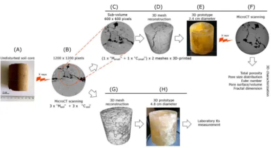
Figure 1 Outline of steps used to obtain soil-like prototypes and sample measurements. 477
Figure 2 2D slices from microCT imaging (M = farmyard manure; C = control) of original soil 478
samples (A1, B1) and soil-like prototypes after the wax removal procedure with ultrasonication 479
(A2, A3, B2, B3) and oven drying (A4, B4). 480
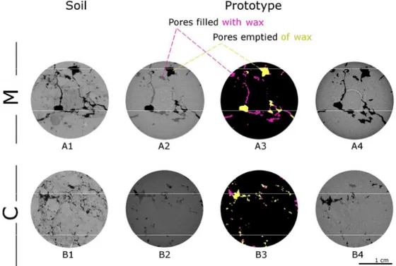
Figure 3 2D slices from microCT imaging of original soil samples (A1, B1) and soil-like 481
prototypes (M = farmyard manure; C = control). Prototypes were obtained in duplicate from a 482
polygonal mesh composed of both 500 thousand (500k; A2, A5, B2, B5) and 10 million (10M; A3, 483
A6, B3, B6) triangles. Grayscale images are composed of empty pores (black objects) and solid 484
material (gray objects). Binary images are composed of empty pores (white) and solid material 485
(black). 486
Figure 4 Pore size distribution estimated by means of X-ray microCT on original soil samples 487
(“Msoil and “Csoil”) and on soil-like prototypes (“Msmall” and “Csmall”) from 3D printing at different
488
mesh accuracy (500k = 500 thousand triangles; 10M = ten million triangles). 489
Figure 5 3D representations of a large soil sample (farmyard manure treatment) as a result of X-ray 490
microCT analysis (A, C; spatial resolution of 40 µm) and pictures of its 3D-printed copy (B, D; 491
spatial resolution of 29 µm). 492
Figure 6 Relationship between saturated water conductivities estimated on soil-like prototypes (K
s-493
large, m s-1) and on the original soil samples by means of (A) experimental (Ks-soil, m s-1) and (B)
494
modelling (KMorph, m s-1) approach.
For Review Only
22
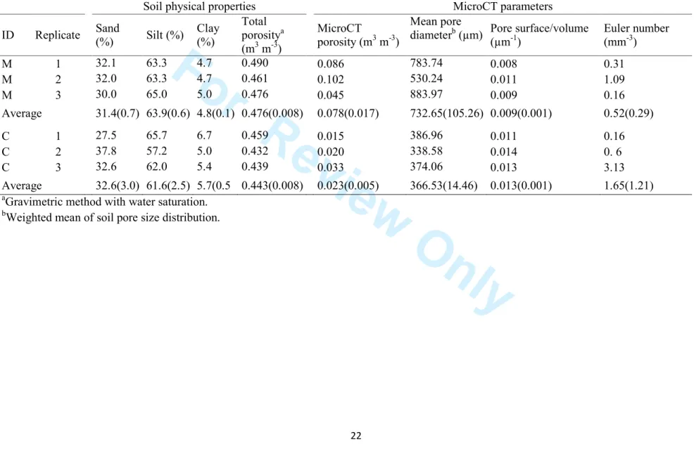
Table 1 Texture and microCT pore morphological parameters of original soil cores (4.8 cm high × 4.8 cm diameter). Standard error values are
496
reported in brackets.
497
Soil physical properties MicroCT parameters
ID Replicate Sand (%) Silt (%) Clay (%) Total porositya (m3 m-3) MicroCT porosity (m3 m-3) Mean pore
diameterb (µm) Pore surface/volume
(µm-1) Euler number (mm-3) M 1 32.1 63.3 4.7 0.490 0.086 783.74 0.008 0.31 M 2 32.0 63.3 4.7 0.461 0.102 530.24 0.011 1.09 M 3 30.0 65.0 5.0 0.476 0.045 883.97 0.009 0.16 Average 31.4(0.7) 63.9(0.6) 4.8(0.1) 0.476(0.008) 0.078(0.017) 732.65(105.26) 0.009(0.001) 0.52(0.29) C 1 27.5 65.7 6.7 0.459 0.015 386.96 0.011 0.16 C 2 37.8 57.2 5.0 0.432 0.020 338.58 0.014 0. 6 C 3 32.6 62.0 5.4 0.439 0.033 374.06 0.013 3.13 Average 32.6(3.0) 61.6(2.5) 5.7(0.5 0.443(0.008) 0.023(0.005) 366.53(14.46) 0.013(0.001) 1.65(1.21) a
Gravimetric method with water saturation.
498
bWeighted mean of soil pore size distribution.
499 500
For Review Only
23
Table 2 3D parameters from microCT scanning of original soil volumes (“Msoil” and “Csoil”) and soil-like prototypes (“Msmall” and “Csmall”). Soil 501
and soil-like volumes were 2.4 cm high × 2.4 cm diameter. Standard error values are reported in brackets.
502 503 ID Sample scanned Mesh a MicroCT porosity (m3 m-3) Open pores/total porosity (%) Mean pore diameterb (µm) Pore surface/volume (µm-1) Euler number (mm-3) 3D fractal dimension Msoil Soil - 0.114 100.00 858.60 0.007 0.42 2.41 Msmall Prototype 500k 0.113 98.97 925.60 0.007 3.54 2.61 Msmall Prototype 500k 0.106 96.36 943.26 0.007 0.82 2.10 Msmall Prototype 10M 0.113 98.71 940.04 0.007 1.70 2.62 Msmall Prototype 10M 0.107 96.32 953.31 0.007 0.97 2.17 Average Prototype - 0.110 (0.002) 97.591(0.84) 940.55(6.62) 0.007(0.000) 1.758(0.72) 2.38(0.16) Csoil Soil - 0.036 100.00 319.02 0.014 0.33 2.25 Csmall Prototype 500k 0.027 90.30 397.66 0.013 0.981 2.40 Csmall Prototype 500k 0.022 79.59 393.33 0.013 0.171 2.55 Csmall Prototype 10M 0.028 86.35 380.00 0.013 0.795 2.38 Csmall Prototype 10M 0.025 76.90 246.21 0.026 1.509 2.46 Average Prototype - 0.026(0.002) 83.28(3.54) 354.30(41.83) 0.016(0.004) 0.864(0.319) 2.45(0.04) a
500k = 500 thousand tringle mesh; 10M = 10 million triangle mesh.
504 b
Weighted mean of soil-like prototypes pore size distribution.
505 506
For Review Only
24
Table 3 Experimental saturated conductivity values (Ks-large, m s-1) estimated on soil-like prototypes (“Mlarge” and “Clarge”, 4.8 cm high × 4.8 cm 508
diameter) and compared with experimental (Ks-soil) and modelled (KMorph) ones on the original soil samples. Standard error values are reported in
509 brackets. 510 511 ID Replicate Ks-large (10-6 m s-1) Ks-soila (10-6 m s-1) KMorpha (10-6 m s-1) M 1 134.94 6.31 5.17 M 2 19.46 2.41 4.13 M 3 30.50 3.41 1.74 Average 61.63 (36.79) 4.04 (1.17) 3.68 (1.02) C 1 N/A 5.27 0.04 C 2 0.23 2.22 0.16 C 3 0.47 1.90 0.24 Average 0.35(0.12) 3.13(1.07) 0.15(0.06)
adata from Dal Ferro et al. (2015).
512 513 514 515 516 517
For Review Only
Figure 1 Outline of steps used to obtain soil-like prototypes and sample measurements. 216x127mm (300 x 300 DPI)
For Review Only
Figure 2: 2D slices from microCT imaging (M = farmyard manure; C = control) of original soil samples (A1, B1) and soil-like prototypes after the wax removal procedure with ultrasonication (A2, A3, B2, B3) and oven
drying (A4, B4). 152x111mm (300 x 300 DPI)
For Review Only
Figure 3 2D slices from microCT imaging of original soil samples (A1, B1) and soil-like prototypes (M = farmyard manure; C = control). Prototypes were obtained in duplicate from a polygonal mesh composed of both 500 thousand (500k; A2, A5, B2, B5) and 10 million (10M; A3, A6, B3, B6) triangles. Grayscale images are composed of empty pores (black objects) and solid material (gray objects). Binary images are composed
of empty pores (white) and solid material (black). 119x160mm (300 x 300 DPI)
For Review Only
Figure 4: Pore size distribution estimated by means of X-ray microCT on original soil samples (“Msoil and “Csoil”) and on soil-like prototypes (“Msmall” and “Csmall”) from 3D printing at different mesh accuracy
(500k = 500 thousand triangles; 10M = ten million triangles). 169x197mm (300 x 300 DPI)
For Review Only
Figure 5: 3D representations of a large soil sample (farmyard manure treatment) as a result of X-ray microCT analysis (A, C; spatial resolution of 40 µm) and pictures of its 3D-printed copy (B, D; spatial
resolution of 29 µm). 118x130mm (300 x 300 DPI)
For Review Only
Figure 6 Relationship between saturated water conductivities estimated on soil-like prototypes (Ks-large, m s-1) and on the original soil samples by means of (A) experimental (Ks-soil, m s-1) and (B) modelling
(KMorph, m s-1) approach. 317x152mm (300 x 300 DPI)