An analytic determination of beta poloidal and internal inductance in an elongated tokamak from magnetic probe measurements

PFC/RR-92-6

An Analytic Determination of Beta Poloidal and Internal Inductance in an Elongated Tokamak from Magnetic Probe Measurements

Joseph Mark Sorci

February 1992

Plasma Fusion Center

Massachusetts Institute of Technology Cambridge, MA 02139 USA

This work was supported by the US Department of Energy under contract DE-FG02-91ER-54109. Reproduction, translation, publication, use, and disposal, in whole or in part, by or for the US Government is permitted.

An Analytic Determination of Beta Poloidal and Internal Inductance in an Elongated Tokamak from Magnetic Probe Measurements

by

Joseph Mark Sorci

Submitted to the Department of Nuclear Engineering in Partial Fulfillment of the Requirements for the Degrees of

Bachelor of Science in Nuclear Engineering and

Master of Science in Nuclear Engineering at the

Massachusetts Institute of Technology

February 1992

@1992

Joseph M. Sorci

All Rights Reserved

Signature of Author:

Certified by:

Accepted by:

Dep29rdnt of Nuclea -Engineering January 17, 1992

Tofssor Jeffrey P. Freiberg ipar ent of Nuclear Engineering

Thesis Supervisor

Professor Allan F. Henry

An Analytic Determination of Beta Poloidal and Internal Inductance in an Elongated Tokamak from Magnetic Probe Measurements

by

Joseph Mark Sorci

Submitted to the Department of Nuclear Engineering on January 17, 1992

in Partial Fulfillment of the Requirements for the Degrees of Bachelor of Science in Nuclear Engineering

and

Master of Science in Nuclear Engineering Abstract

Analytic calculations of the magnetic fields available to magnetic diagnostics are per-formed for tokamaks with circular and elliptical cross sections. The explicit dependence of

the magnetic fields on the poloidal beta and internal inductances is sought.

For tokamaks with circular cross sections, Shafranov's results are reproduced and extended. To first order in the inverse aspect ratio expansion of the magnetic fields, only a specific combination of beta poloidal and internal inductance is found to be measurable. To second order in the expansion, the measurements of beta poloidal and the internal inductance are demonstrated to be separable but excessively sensitive to experimental error.

For tokamaks with elliptical cross sections, magnetic measurements are found to deter-mine beta poloidal and the internal inductance separately. A second harmonic component of the zeroth order field in combination with the dc harmonic of the zeroth order field specifies the internal inductance. The internal inductance in hand, measurement of the first order, first harmonic component of the magnetic field then determines beta poloidal. The degeneracy implicit in Shafranov's result (i.e. that only a combination of beta poloidal and internal inductance is measurable for a circular plasma cross section) reasserts itself as the elliptic results are collapsed to their circular limits.

Thesis Supervisor: Jeffrey P. Freidberg Title: Professor of Nuclear Engineering Thesis Reader: Ian H. Hutchinson

Acknowledgments

First and foremost I would like to thank Professors Jeffrey Freidberg and Ian Hutchin-son for their dedicated teaching and guidance throughout my career at MIT. I would also like to acknowledge those teachers who inspired me: George Webb, Richard Doherty, Doris Shearer, Art Moslow, Jim Guido, and especially Christine Krypel. Thanks goes out to all my friends at the Plasma Fusion Center, including fellow students, technicians, and sup-port staff. A special heartfelt thank you is reserved for Anna Kotsopoulos without whose help this work could never have been completed.

Table of Contents

Chapter 1 Introduction . . . . . . . .. . 1

1.1 Background . . . .. . . . . . 1

1.2 Ideal MHD . . . .. . . . . . . . . . 5

1.3 Notation . . . . 6

Chapter 2 The Circular Limit . . . .. . . . . 7

2.1 Introduction . . . . . . . . . 7

2.2 The Ohmic Tokamak Expansion of the Grad-Shafranov Equation . . . . 7

2.3 The First Order Solution . . . 13

2.4 The Second Order Solution . . . 16

2.5 Summary . . . . . . . 27

Chapter 3 The Elliptic Limit . . . 31

3.1 Introduction . . . . . . . 31

3.2 The Zeroth Order Solution . . . 31

3.3 Beta Poloidal and the Internal Inductance . . . 37

3.4 The Zeroth Order Fields . . . . . .. .. . . 41

3.5 The First Order Solution . . . . .. . . 44

3.6 The First Order Fields . . . 54

3.7 Qualitative Behavior of the Model . . . 55

3.8 Summary . . . . . . . .. . . . . 56

Chapter 4 Conclusions and Suggestions for Future Work . . . 61

List of Figures

Figure 2.1: Idealized Circular Tokamak . . . 29

Figure 2.2: Simple Shafranov Profiles . . . 30

Figure 3.1: Idealized Elliptical Tokamak . . . 57

Figure 3.2:

$,,

02 versus Plasma Elongation . . . 58

Figure 3.3: ,,02 versus Internal Inductance . . . 59

Figure 3.4: ,,1 versus Beta Poloidal . . . 60

Chapter 1 Introduction

1.1 Background

The realization of controlled thermonuclear fusion is one of the Holy Grails of modern physics and engineering. Promising clean, practically limitless energy, fusion is one of the principal hopefuls for future energy development. To this end, fusion research is being conducted worldwide.

A favorite scheme for realization of controlled thermonuclear fusion is the tokamak, a toroidal confinement device pioneered by Soviet scientists. Briefly, a tokamak consists of a toroidal vacuum chamber that loops through powerful magnets, called toroidal field or TF magnets. The TF magnets create a strong magnetic field in the toroidal direction. In modern, high field experiments such as Alcator C-Mod, the toroidal field can be as high as 10 T. In addition to the applied toroidal field, a tokamak realizes plasma confinement by means of a self-generated poloidal field. A powerful transformer commonly referred to as the ohmic transformer is pulsed to initiate tokamak operation. The magnetic flux created by the ohmic transformer links the plasma that is being created simultaneously in the vacuum chamber. The resultant electric field drives a current through the plasma in the toroidal direction creating a magnetic field in the poloidal direction. This current is called the plasma current, henceforth denoted as I,. I, = 3 MA in Alcator C-Mod. The poloidal field created by Ip combines vectorially with the applied toroidal field to create a rotational transform or "screw pinch" equilibrium that has proved remarkably efficient in confining fusion plasmas for brief periods of time.

The difficulty in achieving breakeven, much less appreciable gain, in a fusion exper-iments lies in confining plasma that is hot enough, long enough so that the necessary number of fuel nuclei overcome their mutual Coulomb repulsion and fuse. Typically, mod-ern fusion experiments have T, z 8 keV, ne - 5 x 1020m-3, and energy confinement times

(TE) on the order of 500 msec. Lawson formulated a criterion for achieving breakeven in a deuterium-tritium plasma that is summarized below.

nfeTE DT _ 10 20 m (1.1)

To date, fusion experiments have improved dramatically, by a factor of 104 from initial devices, but still fall short of achieving ignition. Research is ongoing and progress is being made. Several new concepts are being explored in the newer experiments including elongated plasma cross sections, divertors, pellet-fueling, neutral beam and rf heating to name a few.

Crucial in gauging the performance of a given tokamak experiment are two parameters

f3, and fi. O,, known as beta poloidal, is the ratio of plasma kinetic pressure to poloidal

magnetic field pressure. O, has several definitions depending on which convention is em-ployed. For the present calculation the following two definitions of Op will be employed where appropriate.

p)2po (1.2)

Pedge

(P)87rAplasma

A~s,,.(1.3)

(p) is the volume averaged plasma kinetic pressure. B2 /2po can be thought of as the poloidal magnetic field pressure at the edge of the plasma. Equation (1.3) reduces to Eq. (1.2) if the plasma has a circular cross section.

/8, is a measure of how much plasma is being confined for a given edge value of poloidal field. In some sense high fl means better overall plasma confinement and tokamak performance. However, it can be demonstrated that if , becomes too high, that is reaches a certain limit, plasma equilibrium is no longer possible. For the case of a tokamak of circular cross section the O, limit can be expressed thus

_', < 1 (1.4)

ii is the internal inductance of the plasma per unit length normalized to po/47r. It is a measure of the width of the current profile which has direct bearing on the stability of a given equilibrium.

One way in which experimentalists have sought to determine these two important operational parameters is with magnetic diagnostics. For a comprehensive overview of the most commonly employed magnetic diagnostics including Rogowski coils, flux loops, and field coils, see Hutchinson (1987).

Several numerical studies have been undertaken to determine how and under what conditions fi, 3,, and I, can be measured with magnetic diagnostics (Brahms [1990]). Luxon and Brown (1982) while working on Doublet IIa and Doublet III employed a scheme whereby the Grad-Shafranov equation was solved for a particular set of profiles and simu-lated measurements were computed for the 24 one-turn loops and 12 partial Rogowski coils actually monitoring the experiments. These simulated measurements were then compared to the actual data and the differences minimized. Lau et. al. (1985) performed a similar analysis on Doublet III adding 11 local magnetic probes to the diagnostics listed above. Both groups found that the differences between actual and simulated measurements had well-defined minima for non-circular cross sections and that I,, ,, and ii could be deter-mined separately with some measure of confidence. For circular cross sections, only I, and

op +fi/2 could be determined. In a later work, Lao et. al. (1985) demonstrated that in the

circular case ,3 and ii could be separated by appealing to a diamagnetic flux measurement in addition to the other measurements cited above. The validity of such an approach is in doubt however as diamagnetic flux measurements are subject to substantial errors because of a large toroidal field offset.

Numerical work on JET pursued by Brusati, et al (1984), Blum et al (1981, 1985), and Lazarro and Mantica (1988) proceeded along the same lines. Their conclusions were nearly identical with the Doublet III groups'. From magnetic measurements alone, I, and the combination 3p

+

fi/2 could be determined for low 3, in near circular plasmas and

I,f,, and

ei

for non-circular plasmas. A critical elongation of 1.25 was calculated. For plasma with elongations K > 1.25, the measurements were separable.

Much analytic work has been done by Shafranov (1962, 1966) and Mukhovatov and Shafranov (1971). Shafranov demonstrated that to first order in the inverse aspect ratio, E = _{a/Ro, the radial and azimuthal components of the poloidal field outside the plasma}

can be expressed in the following forms.

Be (r, 0) ~ _27rr A - _47r I (. 1 + --2)(#, + )+In -r 1 + 2oaCos 0 (1.5)

r2 2 a _r2

_ _I, 2 Li -i 2Roal

Br(r, 0) ~-

[

('

-)(3,

+ 2 ) +In -- 2J sin0 (1.6)

47Ro r2 2 a r

a is the minor radius of the tokamak, Ro the major radius. A, is the famous Shafranov shift which represents the distance the plasma has shifted outward in order to reach an equilibrium that creates a toroidal force balance. One can determine I from the steady component of Be and A, and the combination Pp + Li/2 from the first harmonics of Br

and Be. Shafranov's model and the studies cited agree.

Wind (1972, 1984) and Brahms et al (1986) applied function parameterizations to the magnetic data analysis on the ASDEX experiment. The goal was to obtain a simple functional form for intrinsic physical parameters of a tokamak in terms of the values of measurements. Again, only OP + L/ 2 _{was determined with good accuracy in the presence} of realistic measurement errors in a near circular geometry.

The objective of the present work is to demonstrate analytically what has been hereto-fore known only computationally. Namely, magnetic measurements are sufficient to deter-mine 3, and Li independently only if the plasma is sufficiently elongated. What follows in the present chapter is a short review of the ideal MHD model. Chapter 2 reproduces Shafranov's results in the circular limit and extends the model further demonstrating how although second order, second harmonic field measurements allow one to separate O, and

Li, the measurements are too sensitive to determine them with any confidence. Chapter 3 addresses the elliptic problem in which (for profiles fundamentally identical to those used in the Shafranov model), the Grad-Shafranov equation is solved explicitly to first order. The resultant magnetic fields available to a hypothetical set of magnetic probes are then calculated explicitly.

1.2 Ideal MHD

For a comprehensive overview of the subject, refer to Freidberg (1987). A few salient points are summarized here.

Ideal MHD treats a plasma as a single, electrically neutral fluid capable of supporting large electric currents. The currents are modeled as being carried by massless electrons while the fluid's inertia lies with the ions. A reduction of the two-fluid equations for electrons and ions to a single fluid equation with these approximations in mind yields the famous force balance equation shown below.

J x B = Vp (1.7)

Ideal MHD models a plasma as having no resistivity. Therefore, Ohm's law can be cast in the following form.

E + v x B = 0 (1.8)

In combination with Maxwell's laws and an equation of state (1.7) and (1.8) can be used to solve for a very wide range of MHD equilibria.

In fusion configurations with confined plasmas, the magnetic lines lie on a set of nested toroidal surfaces called flux surfaces.

Taking the B component of Eq. (1.7) reveals that flux surfaces must also be surfaces of constant pressure.

B - Vp = 0 (1.9)

It is also worthwhile to note that taking the J component of Eq. (1.7) demonstrates that the current flows along flux surfaces and never across them.

Consider the following two Maxwell's equations where the displacement current has been ignored.

V - B = 0 (1.10)

Define the magnetic field B in the following manner.

B = B064 + B, (1.12)

1

B, = 1 VO x 6,0 (1.13)

i is the flux function. Flux surfaces are surfaces of constant b. Combining Eqs. (1.7) with (1.10-1.13) one can derive the famous Grad-Shafranov equation.

= ~1 dp2 - dF

i-poR2 - F-b (1.14)

dO dO

The elliptic operator A* = R2V-

(p).

F = RBk and can be shown to be a free function of flux only.

F =F(O) (1.15)

Likewise for the pressure p.

p= p(O) (1.16)

Equation (1.14), the Grad-Shafranov equation, describes tokamak equilibrium in terms of the flux function 0. Solving the Grad-Shafranov equation for certain prescribed, ideal profiles p and F, one can thus calculate B, explicitly from 0. This is exactly the ap-proach taken in Chapters 2 and 3. In both cases an inverse aspect ratio

(6)

expansion is performed. For the circular case the expansion must be carried out to second order in e. For the elliptical case only first order is required, but the zeroth order solutions are much more complicated. From these solutions, it is possible to deduce the desired information concerning p, ,,, and the magnetic diagnostics.

1.3 Notation

A brief word about notation. Throughout the work, whenever a "caret" appears above any quantity except a unit vector, that quantity is understood to be defined outside the plasma. For example, b denotes the flux function outside the plasma while V) denotes the flux function inside the plasma. Also, magnetic fields are labeled with subscripted direction, order, and angular harmonic. For example, B9,, denotes the first order, first harmoinc magnetic field in the 9 direction.

Chapter 2 The Circular Limit

2.1 Introduction

In this chapter the Grad-Shafranov equation will be solved to second order in the ohmic tokamak expansion. See Shajii et al (1992). Then having explicit formulas for the flux functions ,O I ₁, and b₂, the magnetic fields available to an idealized set of probes are

calculated. The dependence of these field amplitudes on , and fj are sought.

2.2 The Ohmic Tokamak Expansion of the Grad-Shafranov Equation

Consider a circular tokamak as illustrated in Fig. 2.1. The plasma of radius a is surrounded by magnetic probes conveniently located on a concentric circle of radius b. These magnetic probes sample the radial and azimuthal fields during the flattop portion of tokamak operation. Assume that the signals are Fourier analyzed to yield the following information.

B, (, b) = B,1(b) sinG + Br2(b) sin 26 (2.1) Bo(6,b) = Boo(b) + Bo1(b) cos 0 + B0 2(b) cos 26 (2.2) " B,1 is the first order radial field.

* Br2 is the second order radial field.

" Boo is the zeroth order tangential field.

* B9 1 is the first order tangential field.

" B0 2 is the second order tangential field.

The field amplitudes are ordered with respect to the inverse aspect ratio E < 1. That is

Bo_{1 B}Be2 Br2

01 c oce(2.3)

The data yields five pieces of information with which it should be possible to obtain the following five plasma parameters:

*

I, total plasma current.

*

A, the Shafranov shift. * Op the poloidal ,.

" t normalized internal inductance.

" r the plasma elongation.

To obtain analytic expressions for the field amplitudes in terms of the desired param-eters one proceeds as follows.

The MHD equilibrium of the plasma is described by the Grad-Shafranov equation developed in Chapter 1.

A*O = -poR2 - FdF (2.4)

d#k dik

Again p = p(b) and F = F(b), free functions of flux that describe the pressure and toroidal field profiles respectively. For this particular problem assume an ohmic regime of tokamak operation as opposed to the high beta or flux conserving regimes. The regime of operation gives the ordering and appropriate parameters in which to asymptotically expand the Grad-Shafranov equation in order to obtain

4

to the desired accuracy.

Ohmic tokamak operation is characterized by low f, paramagnetic plasma behavior, and q ~ 1 for stability. q is the safety factor where q(r) = Rl-. Ohmic operation assumes that plasma kinetic pressure is confined mainly by a poloidal field generated by ohmic current and not by any magnetic well in the toroidal field.

Expand the Grad-Shafranov in the parameter E, the inverse aspect ratio, where E g

<

1. The ohmically heated tokamak expansion is given by

BP ~(2.5) B4

q ~ 1(2.6)

P ~ ~ 1 (2.8)

P

(ri) ko(r) +ik1(r) cos 0 + 02(r, O) + .. (2.9)

~ e _(2.10)

~ e

(2.11)

01

?P rROBO (2.12)

Choose F2(ik) and p(o) most conveniently and Taylor expand these free functions about

0o.

F2 _{~ R(B2 + 2BoB}

2(b)) (2.13)

P(0) !:- P(0) + _ (01 +02) + 2 (01 + b2)2 +... (2.15)

doo 2 d02

Rewrite the Grad-Shafranov in toroidal coordinates

1 a '7 1 a20 ₂ dp d F 2 1 o sin0 9,0

rrr -r +r 2 002 - -o(Ro+rcos9) do do 2 R COS Or r 80 (2.16)

By substituting the expansions for 0, p(o), F(o) and collecting terms of the same order in C, three inter-related equations are obtained.

co : --a r -90 R 2Bo - po R2 dP(2.17)

rOr Or /d@ do

1 1 a (_ Olk1 01 1 W4o R2B d2B2 /2(, d2p 2r dp\

rOr \ Or) - R0 Or 0 0 1 d#b - oJRo#1+d d-o-) (2.18)

2

r2 ,1(&1 # cos .Xd d2B2 Ro d B

OE

: V2 2 - COS2 + sin2

- R2Bo d 2 - 0B 7 s

Ro -r R2Ro rJo d/o' 2 d0

-

d

2p

(&

d3p

2rb

₁ d

p

r

2 dp ~ o 2 oR (219

- poR 02d02 2 + _ + COS2 Ro (2.19)

Equations 2.17-2.19 shall henceforth be referred to as the zeroth, first and second order equations respectively. The zeroth order equation is a statement of radial pressure balance and the zeroth order poloidal field is given by

1 di~b

Bo = 1o dr (2.20)

Rearranging terms in the zeroth order equation, it is a simple matter to show that j =

Sy. The first order equation can then be simplified and written in the following form

WR-B, dr

1 d (r 1 + ppB_J V _{r? (2.21)}

r drkr dr r2 +Be dr = Be dr

Likewise, the second order equation can be cast in a more tractable form V2_4' 2 - Bo = R(r) + S(r) cos 26 (2.22) Be dr -1 d1 4' /por2 _{dp 2po} r .1 d 1 dp\ 4+ 1 d (o dJ + -- rBe - -1 + 2ROI dr r Bo dr Be dr Be dr 2Bo dr Be dr _ por2 dp 2por d 1 dp $ d po dJ S(r + -krBo - 1 + B dr B-d 2BO dr Bo dr 2Ro dr r Bo dr Bo d Bo dr 2od od

It is important to note that, as the complexity of each equation increases in proportion to its order so does information content. In fact, Eq. (2.22) contains more information than is required to derive the field amplitudes of the particular harmonics being sampled. Since Be2(r) cos20 oc dV;2(r, 0)/dr only, the S(r) cos26 term on the right hand side of (2.22)

will be needed. For all practical purposes R(r) can be ignored for the remainder of the calculation.

To specify the problem completely, the boundary conditions on 4if(a) and ?k2(a, 0)

must be imposed. Before turning to the detailed behavior of 0 on the plasma boundary r = a it is worthwhile to mention that

4'

must be regular at the origin. Whatever the functional form given by the solutions of 2.21 and 2.22, an infinite flux at r = 0 is unphysical and the coefficients of any terms that diverge as r -+ 0 must be set to zero in the region

r < a.

It was mentioned earlier that the boundary of the plasma is circular. That is only true to zeroth order. Let the surface of the plasma be circular with small ellipticity. Assume the surface of the plasma is described by r(0) where

r = a [1 + 2 (1- cos 20) (2.23) The ellipticity is second order in E.

Here it is implicitly assumed that the equilibrium has been so arranged to set the Shafranov shift A. = 0. This is not a necessary condition and has only been assumed for the sake of simplicity.

The surface of the plasma is also a flux surface; that is, 0(a, 6) = const. Therefore, we can Taylor expand Oo(r) at the boundary, add the first and second order contributions to 0, and set the entire sum equal to a conveniently chosen constant.

S+ a dr' - (1-cos26) + 1cos6+4, 2 =0 (2.25)

1dr [ 2

Immediately, it becomes apparent that in order to satisfy the condition that '0(r.(6), 0)

,01(a) = 0 (2.26)

02(a, 6) = -aRoBe ₂ (K - 1)(1 - cos 20) (2.27)

To carry out this calculation analytically it is necessary to use very simple profiles for p(r), J(r) and Bo(r). The following profiles are used to solve (2.21) and (2.22).

2 P= Po(l - ) r < c (2.28) c p = 0 r > c (2.29) Be = Boc - r < c (2.30) C c Bo = BOC- r > c (2.31) r J = J r < c (2.32) J = 0 r > c (2.33)

See Fig. 2.2 for a depiction of these elementary profiles. This very simple model is intended to replicate the behavior of plasmas with dense, current carrying cores, the ratio of c/a being a measure of the peakedness of the actual smooth profiles that are measured in experimental plasmas.

Before substituting these profiles into the first and second order equations, they are used to calculate ti and O, quantities which depend only on zeroth order quantities.

Here, let 3, = (p) . where (p) is the volume averaged kinetic pressure and - is the edge value of poloidal magnetic pressure. Given the profiles outlined above , is simple to calculate.

(2.34)

B2

Now calculate i, the internal inductance of the plasma per unit length normalized to po/47r. Actually the determination of ii is merely a statement of the conservation of zeroth order magnetic energy.

LI2 B rd3V₁sm, (2.35)

2 P J 2yot

i Li /po (2.36)

27rRO / 47r

Breaking up the volume integral into two regions r < c and r > c, and substituting Eqs. (2.30) and (2.31) in the appropriate regions, ii is obtained.

1 = - 2in a (2.37) 2 C a -a

The dimensionless ratio a is a measure of how peaked actual, smoothly varying profiles such as these realized in experiments might be. As a --+ 1 the profiles become flat and as a -+ 0 the profiles become highly peaked. Intermediate values of a can be chosen to approximate a given experimental situation.

Expressions for 3, and fi in hand, one is in a position to solve Eqs. (2.21) and (2.22) and obtain expressions for the field amplitudes to be measured.

2.3 The First Order Solution

Upon substitution of the given profiles into (2.21) in the region 0 < r < c the 01 equation becomes

1 d dO 1 -1 Bec

r r dr 2 -- (1+ 4#,)r (2.38)

Setting the coefficient of any terms that diverge as r -- 0 to zero, the solution of (2.38) can be expressed in the form below

01(r) = -O(1 + 40,)r3 + cir (2.39)

Repeat this procedure for (2.21) in the region r > c keeping in mind that the decaying solutions must now be kept in the form of the solution. Equation (2.21) becomes

1 d d=_{1 =o BC}

(2.40) r dr dr r2 _r

Since 01(a) = 0 the solution to (2.40) can be expressed as

cBoc a 2

41 = -rln- + C2(r - -) (2.41)

2 a r

At this point in the calculation there are two undetermined coefficients, ci and c2.

Application of the and the jump conditions at r = c determine these constants.

J(r) is a step function. dj() is a delta function at r = c. 01 must be continuous at r= c. dJ(r) 1 d dr 1 drBe(r)6(r - c) dr por dr dJ(r) 1 d 2Bec dr - r 6r-dr ~ por dr C dJ(r) _{6(r - c)} (2.42) dr pOC 01(c) - 01(c) = 0 (2.43)

Now examine Eq. (2.21) again integrating over the jump from r = c- to r = c+.

Jc+lId diic+ 01 !r + 2 ~ = C+ 2por dp

(r -)dr - f dr +

J

- c)dr (Be - - )dr (2.44)

The term on the right hand side of (2.44) is continuous. The first term on the left hand side of (2.44) can be integrated by parts twice.

i+ _{+ fc±kldr}

-dr + 2bi (c) = 0 (2.45)

dir ± r

J

r2 c 2c

Applying the continuity of ?P1 at r = c, it becomes evident that the delta function in dJ(r)

requires there to be a step in "' _dr at r = c.

di dP1 _ 201(c) (2.46)

dr dr c

Now apply the jump conditions to the solutions 01 and 1. This gives two equations in

two unknowns.

cBec In a + c2(c - -2 B(1 + 4,)C2 _{- CC= 0 (2.47)}

2 c 8

Ci - c2(1 - _c 2 cBO ₂ Ina -_L 1 4(1+40) (2.48)

The algebra is sufficiently simple that the steps are omitted.

c1 _{= 2a}c =p+ 2 1

₂

_2"

(1 - a2) (2.49)

C2 = (2.50)

7k is now completely determined.

Bec r cBec a2)

01 (r) = ' (1 + 40p)rs - O1 + - 2 r (2.51)

cBcer ln + - + - (r _a (2.52)

,01(r) 2 rna + 2[O+2 2 r

Having 01 and 1, it is now possible to obtain the first order magnetic fields measured by the probes at r = b. After the discussion in Chapter 1, the poloidal magnetic field is

exactly Bp = _{-VO x e6. Taylor expanding the 1/R, substituting the perturbed solution} for 7b = '₀0 + b₁ + 02 + ... and collecting terms of comparable order, the first order fields

are given below.

1 1O#1(r,6) B1, = Ro r 00 B₁,. = - 1 sin 0 _(2.53) Ro r 180 1 07b₀o 1 0 _{1 8 0} Be = - r Cos R Or Ro Or Roar R! Or 1 &?ki

1

Bio = [ ON-1r -jBe(r) cos 0 (2.54)

Substitute (2.52) and (2.31) into (2.53) and (2.54). Evaluate the expressions at r = b.

I.~4 /.Op-e 1)( 2₎

_bl

($±l

=2+ )(1 -) +In-i (2.55) 4,rRo 2 b2 _a I 1)( + a') b 47rRo2+ (2.56)

Note that both field amplitudes only specify the combination O, + - uniquely. They give 2

the same information. It can be shown that taking the combination b 1 = Be1(b) -lB, 1(b)j

subtracts out any shift information wrapped up in the first order fields. This combination is included here for reference only as the Shafranov shift Aa has already been set to zero for convenience.

1 = l [1 2 (. + 1 (2.57)

Again note that only the combination O, + - can be found from the data. The first order field measurements do not specify fl, and fi separately. Although it would seem that having determined the plasma current I, from zeroth order measurements and knowing the geometry, the two field measurements, B1, and B16, are sufficient to determine f3, and

ej

separately, they are not. O, and i; relate to the first order measurements in a linearly dependent fashion.

2.4 The Second Order Solution

Next, turn to Eq. (2.22) for 02. Perhaps the second order field measurements can supply the additional information necessary to find fl, and fi. Focus on S(r) in the region r < c. Substitute the expression for 01 in that region and the given profiles.

1 do, =- 1 - 2 dp 2por 1 j d (1 dp\ + d ( _po d

S(r)=j 2Ro Idr ~ r r~r Bo(r ) dr Be B- dr \ d Tr 2B, Tr BdrBe Bed}dr Since != 0, the last term on the right hand side vanishes.

1 = 2 + 4 2 - - 2 or2 2R- 8R c 8c cB0,r \ 2 S(r) = 1

5

(1

+40)r2-

r2 + 2flop 2 2R0 4c c Boc

J

S(r) = Be 1 ,-1+2 r2 2ROc

4

B S(r)= 33 p- r2 S(r) = 3Be - 1 r 2 r < c (2.58) 2ROc I P-45

For the purpose of calculating the amplitude of the second harmonic that appears in second order, Eq. (2.22) becomes

v202 = 3Bec (op)r2 cos 20 (2.59)

A solution of the form 4'2(r, 9) = 4'2(r) cos 20 is sought. Substituting this form of the solution into (2.59) converts a second order partial differential equation into a second order linear ordinary differential equation which is trivial to solve.

d20k2 +di,b 2

4

_3

Bec

2 (.0

+

-2 202 = (p - 1r2 (2.60)

r+dr 2 r 2 Roc

k

4

Immediately one can write down the solution in the following convenient form

The same procedure is followed in order to find '02(r, 0). This time 01(r) and the

appropriate profiles for r > c must be used to compute S(r) in this region.

_ d, 1 por

2 _dp

_2po ri 0 d ( 1 dp< + d2 t

J'

S(r) = - - -dr) 2(_r 1 po V

2 l r r _rBe(r) - Be(r) dr -Be (r) dr W9 dr) 2B,~ dr 'Bo(r) dr

J

Again the last term on the right hand side vanishes because J(r) = 0 for r = c. Also the pressure p(r) as well as its derivative d _di' are zero in this region. S(r) simplifies greatly. S(r) = {d -j '' - rBe(r) S(r)= 1 cB ra + cBec n +C2+C2a 2 2c a+ 2 - Br-c 2Ro 2 ar 2 a r2 2 a r2 r S(r) = 2 2c2 -1 2Bcc _{l+ i} - 1] a2 _Becc} S(r ) - 2Ro 2 O 2 2 r2 2 S(r) - Bc + r > c (2.62) 2Ro Ilp 2 r2 2

For the purpose of calculating the amplitude of the second harmonic that appears in second order in the region r > c, Eq. (2.22) becomes

v

2 = O{ + 2 (2.63a)

A solution of the form 42 (r, 9) = ' 2 (r) cos 20 is sought. Substituting this form of the

solution into (2.59) converts a second order partial differential equation into a second order linear ordinary differential equation.

d2 2 1 d02 4k2 Bocc [( 2 1

dr2 _{+ r dr r}2 _{- 2Ro O}

₊

_{2 r2 22}

The solution is expressed most conveniently below.

2(r) =) - 2 + a2+ In + b2r2 + (2.64a)

At this point in the calculation of 0, there are three undetermined coefficients bl, b₂ and

b3.Application of the jump conditions at r = c and the boundary conditions at r = a will

fix these three coefficients. Up to this point in the analysis, the microscopic details of the calculations have been omitted as they were for the most part trivial. From this point on however the algebra becomes both subtle and cumbrous and therefore it is worthwhile to include each step.

First, determine the jump conditions on

b

2 and '2 across r = c. Again, return to Eq. (2.22) and rewrite it in the following form.

d2'02 1 d02 4 po V

dr2 +r dr r2_{02 Bo(r)dr}

1 [d@1 1 2 dP 2porol d 1 dp 02 d ( po dJ

[ - -1i -01 - II)

2Ro dr r - rB₉(r) - dr Be(r) dr Be(r) dr 2B,(r) dr \Be(r) dr

}

(2.64b) Considering the step behavior of J(r) and dr, one finds that the jump conditions can

be determined quickly if '2 (r) near r = c is expressed in the following form

'02(r) = AJ(r) + Bp(r) + ' 2(c+) + smooth functions -+ 0 as r -+ c (2.64c)

Substitute this form of 02(r) into (2.64) in order to determine the constants A and B.

A d+A-- A J + B - B 11 - _ P 2(c+

rr

, dr Be (r) dr d2 Bo(r) dr Bo(r) dr

1 [ 2por#1 dp + oV 1 d2J 1 dJ dB_{9 (2.65)}

2Ro

[

Bj(r) dr2 _{2Bo(r) \Be(r) dr2 B (r) dr dr}

[d2J ldJ _po dJ'

rd

2

p

po dJ

]

o J

A dr2 _{r dr Be + B} [dr2 B dr Be dr 02(C) 1or1 d2p 1ok 2J 1dJ Vpo dJl

RoB 2dr2' 4RoBi [dr2 _{+ r dr Be dr .}

Find A and B in terms of 42, Bec, Po and the normalized first order flux 2 4 A = t0C-2 (2.66) 4Ro1 d2_{p 11o dJ -poc,1 d2p} dr2 _{Bec dr} 2 RoOc dr2

Recall J = JoO(c - r) and 9 = - 26(c - r) where B(c - r) is the heaviside step function.

dr C

Therefore, can be written in terms of d.

d cJo dp _(2.67) dr 2po dr2 d2p IO (_cJo d2p - poc d2P dr2 _Bee 2_{po /} -r2 RoBOc 2 /IOCJO - 11oc;a

B

= -j-;- 12-2B'po RoBOec

Rewrite B evaluating Bec with Ampere's law around a circular contour at r c.

pOJ 2B (2.68)

C

B = k2 - Poc34' (2.69)

pO RoBoc

The reason for writing i 2(r) in the form of Eq. (2.64b) now becomes transparent.

02 - 02 = -A Jo (2.70) d4 2 d02 = -Bdp (2.71) dr dr dr 4-2 2Boc poc 4 poc 4RO 2 - 02 = - c'Bor2 (2.72) 2Ro d -d2 d0 2 2po

(

2 PoC3V'1 dr dr c P R Bo c d 2 d 2 - - Boc2,2c (2.73) dr dr c

O

At this point in the calculation the jump conditions at r = c given by Eqs. (2.72) and (2.73) and the boundary conditions on '2 at r = a given by Eq. (2.27) completely determine the three unknown coefficients bl, b2, and b3. Equations (2.72), (2.73) and (2.27) can be written

as follows.

S-- 1

Aa

(

+ -In a 2 - bic2_- P( , - )c" = _ ____141?11 2b2 c - 2 C3 8R-cln -2c 2B , - 2 b2a 2 ₊ -a2 b2

+

)

[(b

2cC2

2

cBec Aa2 SR0

+

- 2b1c - Bec 2 2 2Ro c.Boc 8Ro

₍

_Aa2 ₊ 2 Ina)] =

2

Ro(m - 1)

Write these equations in matrix form.

b2C 2 + b b1c 2 = c1 C2 2b2c 2 - bi C2 = C a b2a 2 + b3 = + cBe (Aa 2 SRo + R(clna+ c) + -Ina) 2 c3Boe c3_Bec c2= _2R0' ci=c3Bec C =c oc 2R] 2#,5+ _{1(lna + )+ 1(O,} -S 1 _{+ 1 1} 1 Aa2 20,461 + 4na++(# 4 C2

2+

Aa2+

1In a + 1(Op - )1

I(n - 1) - A

Solve for b2c2, b3/c2, b1c2. That is, write the system of equations developed above as a single matrix equation.

1 1 2 0 a 2/Cc c2/a 2 -1] b2c2 ] C

1

-1 b3/c2 = C21 0 _ b₁c2

I

C3

c1, c2c3 are known and given by (2.75-2.77). Repeated application of Kramer's rule to

(2.78) wll solve for the column vector on the left hand side. However, since the present

b2c 2

₊

C2 cB-SRo 2c 2Bc -c C2 - _Ro -fp₁₂ + Bec+2Ro2 (- _4c 1 4 A a2 + 4 c2 +1 Ina]8 i (2.75) (2.76) (2.77) (2.78)

calculation is aimed at determining b 2 0(b) and B2,(b), it will only be necessary to solve

for b2 and b3. The second order magnetic fields are uniquely determined inside the plasma

but are not of interest here.

It is a simple matter to calculate the determinant of the 3 x 3 matrix on the left hand side of (2.78). Then, two applications of Kramer's rule give b2 and b, completely

specifying i2--1 (a4+ c4) (2.79) a2_/c 2 _c2_/a2 _{0 a} c C1 1 -1 2 Db2c2 = c2 0 -1 =-[c3 + -(c 2 - c1 )] (2.80) c3 c2

/a

2 0 a b3 1 c -1 a 2

D

= 2 c2 -1 =-ca - -(c2 - cl)] (2.81) c a2/c 2 c3 0 C

Note the combination c2 - ci appears in both (2.80) and (2.81).

coc B -[ + n 1 1 A a2 C2 -C 1 = 2RL _+2(na- + C2 2 4 62 4 4 +1 4 c2 8 4na 4(, C2 - c 2oB 2 _- 20 + 1 1 n a

+

g1 (2.82) At this point in the calculation it is possible to obtain analytical expressions for the second order field amplitudes measured by the probes. Again the poloidal field can be expressed exactly B, = IVO x eo. As before, substitute the perturbed solution for 0 = Oo + 01 +

02... and Taylor expand the 1/R

l 8

r R 8

1

29-

1 _ b2cosi b

B bR 1 sin

+ 22 sin 2

1 -cos ... Keep only second order terms with sin 20 dependence.

1 bej (b)

Repeat the same procedure to find B02(b). 1R O Be_{2 - R Or} cos 2 0 Cos 6+ $02(b) =

1

[ 2 Ro IOr b O 9r 2Ro Or

b

2 ₈₀₀

+

2RR-0 OrJ

Turn to Eq. (2.83) and evaluate each term. = 2 _{cBc blnb +} cbBe c

[

n b ₊ I R in + b(1 - ) 2 (1 - )] = -_ _ In

-

+ (1 - a 87rRo Ro I a T2' b2C2 ( ₊ b3 c2)(b - cBe' (Aa 2 8Ro + -In 2 b)]aJ bRoV)2(b) = Ta + Tb Ta =2 [bb2c2 + C2b3 T- cBec2 I- In b+ A-12 a 2j

Evaluate Ta, then Tb.

Ta =

2

T = aDbRo -2 Ta = _DbRo [(-C3 - S(C2 -ci)) + C2 -b4 + c 4 b2C2 + 2 C (C2 - l ] - Cl)] b C+bba(C2 - Cl) b2C2 C3

+

a2b2 1 J

302= 1

EOr

NO

+

Cosr + b2bCos 29

cR s 0 (2.84) 1 2 1(b) 1 _(b) 2 1(b) 2R₀ 2(b)= 2 bRo (2.85) where (2.86) (2.87) (2.88) b2 )(C

T

= -2 b + c4 C.BO' : (K 1) + 1a 2 = DbR₀[b2c2 2Ro C2 4 C2 + - a4 C3Bec +a2_b2

_2Ro

- 2039 1

+

Ina + Qbi 8 p1I b a2c2 c2

T

27rRO RO a4 ₊ C4 b2

[

b4_±C4 (+!2 b2c2 1 + 1)+4 c2 V- a 4 + _{a2 V} Tb = -87rRO R0 2 1 1 b # : j + 8 n P (1 In b 2 a + ) Recall from Eq. (2.66) that = (C) .'i

1 Ina + (1 a 2

C2

B,.₂(b) = - 2 >1(b) + Ta + T

Define the dimensionless quantity b,,2.

br2 = i, ₂(b) b POIp/87rRo Ro b b,2 =- In -a a2 T21- A l b - 1 In -2 a a2 _4a2 c2 c2 be + c4 2 _{+ 0 + c4} 2 b2c2 R2 la 2 :g (r - 1) + 4--2A 4a2c2 c2 b- a4 -1 1 + 44Z a2_b2 _{-2,3,i/ + In a + 4,]} 4 4 2 (C -2 a4+C4bV bV

K-1

a

2

1

_b

4

_a

4

_C

4

_T2

2

1

3pl

1) + A +4 b - 2a,4+ + In a + 1 98 4 (2.94) For the interesting case when b = a, that is when the probes are on the plasma surface, b,2 reduces to the following simple form.

br2 = 42 (K - 1) a2 b = a (2.95) (2.89) (2.90) (2.91) (2.92) b2 =- In -2 a (2.93)

It is also useful to examine the opposite limit b

>

a, the case when the probes are located far away from the plasma surface.

3 b - 4b4a2 _{1 [ (2 1 2\ 4c}4 b,2;-2

Ina

A 4 _{+ C}4_)b2 _{bF [R}

_{_1}

4JaIa 4 _{+ C}4 - 2,#1p + 8Ina + b,,2 ~ In b 2 a +44 _R( - 1) + 4+4 a2 +4c 4 2 20 + 1Ina + -+a4 + C4 1t-8J 4

Now unfold the algebra in Eq. (2.84) in order to obtain analytic expressions for the second order second harmonic tangential field.

O2

[Or

b Or 2R0 Or + b2 b1 2RO Or

Ib

b

b2 _NVO 2R3 Or b T2 bRgOj T2 _r T3 M RoOr _b T _ /10 b -47rRo R₀ T2= _{- 2JO} b [

'(In

(l+

1

)

+

(1+

)

cBoc

b cBr b 6 2 ] T 2 - b 2 cIn- b+1+ (1±-a 2RO 2 [ a P~ 1[c-e + b, T = -c-(bn Ro[8Ro a 2 T3 = I-OI (n l67rR0 R0 a

T

3 = 16 b (In -b 167rRo R( a 2 DbRo + 1) 2 +1) 2 rb2 c2 2C3c - (C2 )+2b2b

-+

[b2C2b b3C2 +Ro C 2 C2b

j

C2 - Cl))+ ( a2 + C b > a (2.96) (2.97) (2.98) (2.99) (2.100) (2.101) -ci))] B20 (b)= Ro

2' plOI b b 1 T3 67 (In -+ ) l67rRO Rolf±) 2 b 2 _C2 _{b2 a 2 )C} C3+(-~ + DbRo I C )C + + )2 -T3 =_ 1 I b (In

b

+

1

167rRo Ron + 2

2

[b

4 _{_C}4 _C3

_Bec

_(RO2

_~a 2 _{b + a}4 _C3

_B,9

_a,+

a

pI b [a2 c4 - c4 (K- 1) + - -R I2 27rRo R [b2 a4+ c4 c2b2 c2 4 c2 a2 c b+a 4 14 1)] l2rRo Ro la2 + a0 c ba2

(

-2 2R1 Ina

+

) -~( 2p) - + a4rR0R [C ±4 KK()1±8i

4)]

T-324+c4 I 1 + n

+po

(2.102) +₂ (b) = T1+ T2+T

Define the dimensionless quantity b02.

b 62 = f 02(b) b

(2.103)

pOI/87rRo RO

Combining terms and normalizing properly b02 can be written in the following form.

3 3 b

1a

2 _4a2 _b4_{-_C}4 _{1 1a} 2

be2 =- - In -(1A+ )A _ + + (r. - 1) + -T2A (2.104)

4cb4 _a- 14 V4

+ 44 (Vk2 - 2i 1 + In a + )

Before examining be2 in the limits b = a and b

>

a, it is necessary to simplify b,-2 and b0 2 once more.

Combine A terms in (2.94) and (2.104). a

b

4 + c ₄ b,2 : _{1+ K 4} + 14 b82 : _b (b - a4 ) c4 (W - C4) b4 a4 b4 - C4 + T4 a4_c4 I

a

2 _(b4 _{+ a}4_{) c}4

-

(a4 + c4) V Simplify A. 1 1 A ,+f 2 4na--1 201 + In a + P₄ + ₄ - 2, 1 + i can also be simplified.

- 1

(

- In a

Rewrite b,2 and b02 using (2.105-2.109).

a b /b 4 +a 4_{) a 4 (-\} In- +41I 2 a - a4 +c 4 b4 \ E2 b 3 a2 (b4 - c4 a4 n -+- A+4 44 a 4 b2 _~a 4 _{+c b'} (K-1)

(b

4 + a4 +4a4+c4) 8 16 *i+ l na+ (2.110) 3 8 (2.111) Consider b

>>

a, that is when the measurements surface is far from the edge of the plasma.

3 b 4 br₂ -- In - + 2 a 1+ a 2 3 b b02 ~ -- In -2 a 3 4 4 1+ a 2

(-E2

)

( 2 ) + 4 2 -2 _ + a41 _r+v4 -2,1 + 4a2 + 14 3 ii - Ina + -8 161 -2 _ _{3 1} #1 -2Ppji + -In a + - 1

Notice that b,2 and b82 have exactly the same dependence on K (also unknown) O,, and a. Hence, profile effects cannot be separated from the ellipticity for measurements of B, 2 and b82 far away from the plasma edge. p and fi are still not uniquely determined.

(2.105) (2.106) Also (2.107) 16 3Ina + 8 (2.108) (2.109) b-,2

3

3

6 2 = --₂ 1-(2.112) (2.113)

1

= ₁ +4 bd - a4\ C4 ro-2 -+ 4 a+ C4 4 #1 2,

Consider b -+ a, the opposite limit, when the magnetic probes are placed close to the plasma edge.

bh2 = 4 (K 1) (2.114)

b02 = 3 - A + 4 (1 + a4) 2 1) + + 8a4 2- 2flp: + Ina +

]

(2.115)

Consider (2.114) and (2.115) in the limit a ~ 1 flat profiles. Let a = 1 - 6, 6

<

1.

- [-b + A(1 - 1 + 26)] = (2A - 1)b (2.116) Rewrite (2.114) and (2.115) in this limit.

b,2 4(K-1) (2.117)

3 166 4-1 1 3 _1

b = 42 - A + 2 E 2 +4+(l - 2, _{(2A - 1)6]} -1 3 _1(218

be2 = 1 - A + 6 [8 - 4(2A - 1)(A - )(2.118)

For flat profiles, a ; 1, b,₂ gives no information about a and hence ii and b0

2 gives

information but is is a small correction of order 6 compared to 1 - A, already a small quantity. This will be difficult to measure in practice.

Hence, even resor ting to second order magnetic field measurements does not uniquely specify ti and 3, in the circular limit.

2.5 Summary

The equations of interest are summarized below.

-

-= _{$1= 47rRO} poI[1, [1_ 2aQ2 (O) (257)

V 2 # 2 (.7

For b

>>

a

b,-2 3 b 4 ( - 1 4a2 -2 -2 i+ 3 1(2112)

3

b

3 4(K - 1 4a2

_r-2

_-2113 b82 3- In - + - + ( + +, - -23 +a + Ina + (2.113) 2 a 4 1+a2 ,2 + 4 8

6

For b -+ a b,-2 = 4(KC1) (2.117) b02 = 1 - A\ + 6 18 K - - 4(2A - 1)(A - 1)(21)

It has been shown that for plasmas with circular cross sections with small, second order ellipticities, first order, first harmonic field measurements determine only the combination

fl,

+

£i/2.

Second order, second harmonic field measurements when taken far away from the plasma, cannot separate the ellipticity from the profile effects. The same measurements if taken close to the plasma edge depend so sensitively on already small quantities that experimental errors invalidate them. Therefore, we conclude that even appealing to second order, only the combination r + ii /2 is available to practical magnetic diagnostics for near

C a b RO

Jo

PO

c

Be

a

Figure 2.2: Simple Shafranov Profiles

Chapter 3 The Elliptic Limit

3.1 Introduction

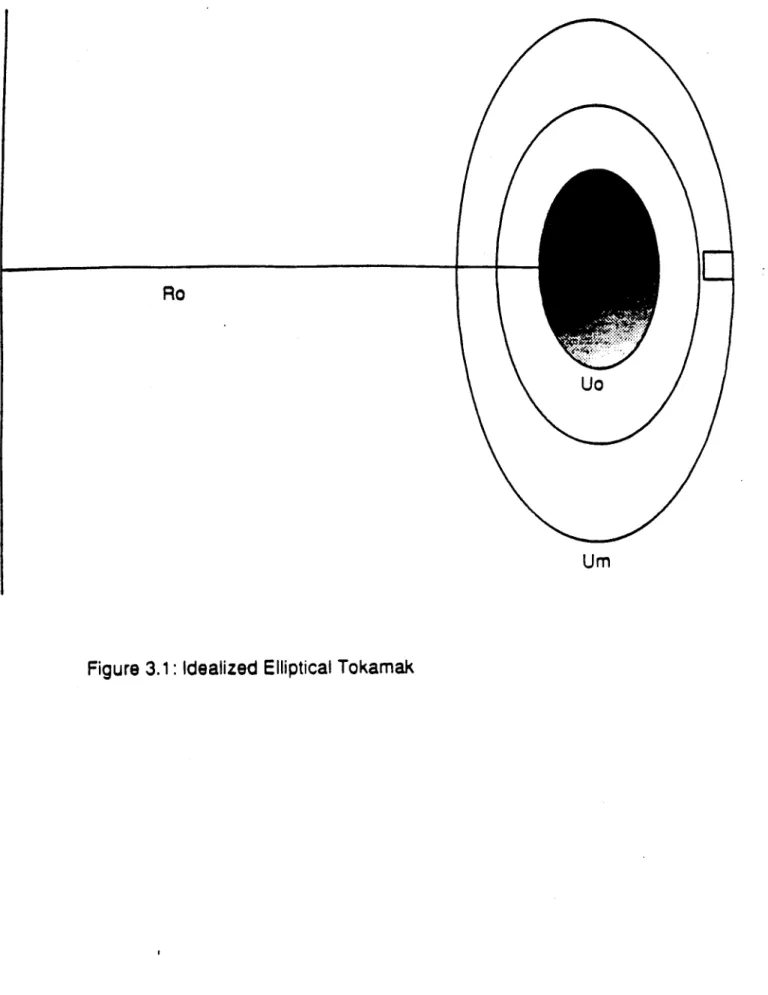
In this chapter the Grad-Shafranov equation will be solved to first order in the ohmic tokamak expansion. Then, having explicit formulas for the flux functions ?Po and b1 outside the plasma, the magnetic fields available to an idealized set of probes are calculated. The dependence of these field amplitudes on p, and ii are sought.

3.2 The Zeroth Order Solution

Consider a tokamak of elliptic cross section as illustrated in Fig. 3.1. An elongated plasma limited at a horizontal distance Xb from its center is surrounded by magnetic probes conveniently located on an ellipse characterized by the elliptic coordinate urn. Before proceeding further, it is useful to review the system of elliptic coordinates that will be used throughout the calculation. The elliptic coordinates are u,v, and 4. 4 is the familiar toroidal angle. Surfaces of constant u are ellipses and v is an angular coordinate varying from 0 to 27r. The transformation from rectangular coordinates to elliptic coordinates is given below.

x = csinhucosv (3.1)

y = ccoshusinv (3.2)

c is a length factor that for the remainder of the problem will be considered determined

by the actual dimensions and ellipticity of the measurement surface. Solving the two transcendental equations that appear below, knowing the height ym and width xm of the measurement surface, uniquely determines c and urn.

Xn = c sinh ur (3.3)