Analysis of linear homing missle control systems

ANALYSIS OF LINEAR HOMING MISSILE CONTROL SYSTEMS by

John Michael Gallagher, Jr. B.E.E., Rensselaer Polytechnic Institute

(1951) F

SUBMITTED IN PARTIAL FULFILLMENT OF THE

REQUIREMENTS FOR THE DEGREE OF 0

A

MASTER OF SCIENCE at the

MASSACHUSETTS INSTITUTE OF TECHNOLOGY (1954)

Copy No. j of 6 copies Each copy contains viii pages and 103 pages

SECURITY NOTICE

This document contains information affecting the national defense of the United States within the meaning of the Espionage Laws, Title 18 U.S.C., Sections 793 and 794.

Its transmission or the revelation of its contents in any manner to an unauthorized person is prohibited by law. Signature of Author.

Signature redacted.

Departmentaf Electrical Engine 'ring, anuary 18, 1954

Signature redacted

Certified by... ... ,,...

Signature redacted

Thesis 1upervisors

Accepted by. . . . . . .

Chairman, Departmental Committee on Graduate Students

/.

'- aAc9

LJNCLASS~ILED

\ASS

0 4 4 6 0 v a * v

r:77----.- ., I '' MR

UpCLASSWFp)

1.1.

1.2. Background of the Missile Problem . . .

1.3. Derivation of Linearized Trajectoxy

Equation. . . . . .

1.h.

Equation. . . . . . ... .o .,.o 1.41. E - Aiming Error . . . . 1.42. T - Target Maneuver. . . . . . . .

1.43. D - Constant Drift. .

1.44. P - Impulse Drift.

1.45. General Normalized Trajectory Equation . . . .

CHAPTER 2. ROOT-LOCUS METHOD. . . ...

2.1. General Discussion of Root-Locus Method .

2.2. Characterizing Parameters of Time Responses 2.3. Root Locus of General Normalized Missile

System-.**.*.*.,,, . .. . .. .. .

2.4. Quadratic Missile Control Systems . .

2.5. Cubic Missile Control Systems . . . .

2.6. Quartic Missile Control Systems . . .

UC L T A - r% 1I E M ASS 1FL.ED

UNCLASSIHED

3

6

UNCLASSIFIED

r

_4.

IMPULSE RESPONSE METHOD. . . . . 3.1. Derivation of the Impulse Response Transfer

Function . . . . . .* * * . * * . * * 3.2. Applications of Impulse Response Method. SUMMARY AND CONCLUSIONS. . . . .

GLOSSARY. . . .

BIBLIOGRAPHY. . * * . . . * . * . . . . DEVEIDPMENT OF THE ROOT-LOCUS EQUATION. . .

GAIN AND FREQUENCY CROSSOVERS . . . .

THE RELATION OF THE EFFECTS OF DIFFERENT PER-TURBATIONS UPON MISS-DISTANCE CURVES. . . . DERIVATION OF TRANSFORMED MISS-DISTANCE CURVE

FOR UNDERDAMPED QUADRATIC MISSILE SYSTEM. .

. . . . iii Page 66

66

94

UNCLASSIFIED

UNCLASSIFIED

iv

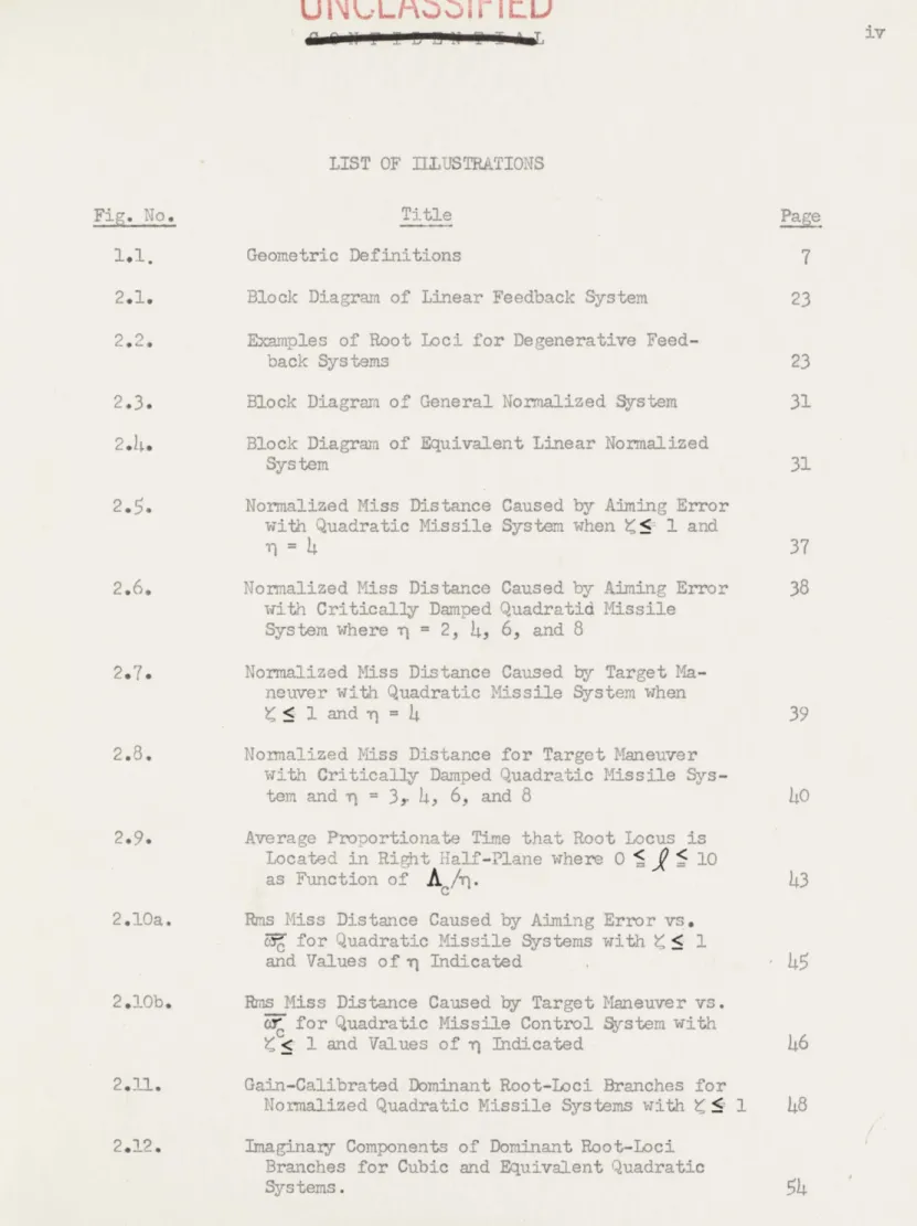
LIST OF ILLUSTRATIONS

Fig. No. Title Pg

1.1. Geometric Definitions ₇

2.1. _{Block Diagram of Linear Feedback System 23}

2.2. Examples of Root Loci for Degenerative

Feed-back Systems 23

2.3. Block Diagram of General Normalized System 31 2.4. Block Diagram of Equivalent Linear Normalized

System 31

2.. Normalized Miss Distance Caused by Aiming Error with Quadratic Missile System when (S 1 and

*

= 4

2.6. Normalized Miss Distance Caused by Aiming Error 38 with Criticaly Damped Quadratid Missile

Sys tem where n = 2,

4,

2.7. Normalized Miss Distance Caused by Target Ma-neuver with Quadratic Missile System when

Y 5 1 and 4

= 39

2.8. Normalized Miss Distance for Target Maneuver with Critically Damped Quadratic Missile

Sys-tem and r = 3,. 4, 6, and 8 40

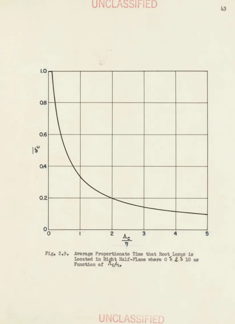
2.9. Average Proportionate Time that Root Locus is Located in Right Half-Plane where 0

j

-as Function of

Ac/rn.

₄₃

2.10a. Rms Miss Distance Caused by Aiming Error vs. Zc~ for Quadratic Missile Systems with Y : 1

and Values of n Indicated ₄₅

2.10b. Rms Miss Distance Caused by Target Maneuver vs. o _c for Quadratic Missile Control System with

S< 1 and Values of - Indicated 46 2.11. Gain-Calibrated Dominant Root-Loci Branches for

Normalized Quadratic Missile Systems with ( i 1 48 2.12. Imaginary Components of Dominant Root-Loci

Branches for Cubic and Equivalent Quadratic

Systems. 54

Fig. No.

U NCLAS*iI

ED

UNCLASSIFIED

.. L LI U U .1. .I .L _

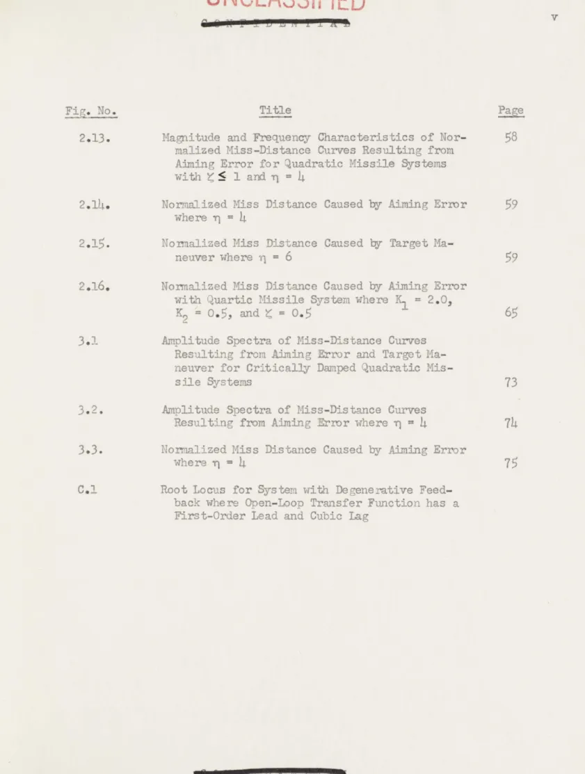
Title

Magnitude and Frequency Characteristics of Nor-malized Miss-Distance Curves Resulting from Aiming Error for Quadratic Missile Systems with ( i 1 and _{- = 4}

Normalized Miss Distance Caused by Aiming Error where -r = h

Normalized Miss Distance Caused by Target Ma-neuver where r = 6

Normalized Miss Distance Caused by Aiming Error with Quartic Missile System where K₁ = 2.0,

K2 .5, and .5

Amplitude Spectra of Miss-Distance Curves Resulting from Aiming Error and Target Ma-neuver for Critically Damped Quadratic Mis-sile Systems

Amplitude Spectra of Miss-Distance Curves Resulting from Aiming Error where = 4

Normalized Miss Distance Caused by Aiming Error where T- 4

Root Locus for System with Degenerative Feed-back _{where Open-Loop Transfer Function has a} First-Order Lead and Cubic Lag

2.13. 2.14. 2.15. 2.16. 3.1 3.2. 3.3. C.1 V Page

73

74

UNCL!

Si'Fp

~~ i

AT

ANALYSIS OF LINEAR HOMING MISSILE SYSTEMS by

JOHN M. GALLAGHER, Jr.

Submitted to the Department of Electrical Engineering in partial fulfillment of the requirements for the degree of Master of Science.

ABSTRACT

The primary factor in the evaluation of missile-control-system operation is the value of miss distance achieved when the missile attacks a moving target. A linearized trajectory study for the pur-pose of evaluating generally the operation of quadratic missile con-trol systems guided by proportional navigation was recently performed on the M.I.T. Flight Simulator. The results were made general by the

use of normalizing techniques that greatly reduced the number of parameters involved. The responses of the quadratic missile systems were obtained in the form of curves of normalized miss distance versus time of flight. Several such curves were also obtained for

cubic and quartic missile control systems but the data by necessity were not nearly as complete as that for the quadratic systems. In

this thesis a method whereby the miss-distance data for the quadratic missile systems can be extended to higher order control systems is developed. This method is applicable only to linear missile control systems and resulted from the study of the possibilities of applying the root-locus method of analysis to linear feedback control systems

UINLLA

sIFIED

with time-varying gains conducted in this thesis investigation. The techniques of linearizing and normalizing the missile tra-jectory equation are reviewed in this thesis as well as the founda-tions for the root-locus method of analysis.

A method for obtaining the transformed expression of the

nor-malized miss-distance curves in terms of missile system parameters is also presented.

Thesis Supervisors and Titles,

Richard Crittenden Booton, Jr., Sc.D.

Lecturer, Departmrent of Electrical Engineering

William Kirby Linvill, Sc.D.

Associate Professor of Electrical Engineering

Q n3 ITT

UNCLASSIF!ED

ACKNOWLEDGMEIT

The author sincerely appreciates the encouragement and many helpful suggestions offered by his thesis supervisor, Dr. R. C. Booton, Jr., during the supervision of this thesis. He also wishes to express his gratitude to N. W. Trembath for

the time contributed by him in numerous discussions of the thesis problem and to Prof. W. K. Linvill, his co-supervisor for his reading of the thesis. The author is indebted to the personnel of the Dynamic Analysis and Control Laboratory, without whose aid this thesis would not have been possible.

In particular the author wishes to thank the analysis group for computational aid, the drafting department for preparation of the figures, and Miss Jeanne O'Brien for proofreading and

typing the manuscript.

viii

U

JJL S

,

E P

Ir

CHAPTER I. INTROIJCTION

1.1. General.

There are in existence at the present time three commonly known methods for the purpose of analysis or synthesis of linear constant-coefficient feedback control systems. These three methods are the frequency-response method, the error-coefficient method, and the root-locus method. Each of these methods has its various advantages and disadvantages, and the selection of one in preference to the 'others is largely a function of the particular problem at hand. All three methods, however, have a common origin: that the relationship between any two quantities within the control system can be written in terms of a differential operator with linear constant coefficients. The different methods owe their existence to the variety of ways these differential operators can be manipulated in order to obtain the desired results.

A large number of feedback control systems exist for which at least one of the relationships between quantities within the system is defined by a linear differential operator with time-varying coefficients.

It is the purpose of this thesis to investigate the possibilities of adapting one of the afore-mentioned methods of analysis to a feedback control system whose loop gain varies as a monotonic function of time. The root-locus method, by virtue of its basic nature, appears to the author to be the most logical method of analysis to apply to this

type of system.

Numbers refer to references listed in the bibliography of Appendix B.

A widely studied example of such a feedback control system is a guided missile homing on a moving target by the use of proportional navigation control. The informative part of the response of this

control system, especially from the standpoint of evaluating primary effects, is the value of the response at a particular time to an input disturbance applied at some known time in the past. This value of response is commonly referred to as the miss distance.

Analytical techniques have been developed for handling this particular control system on the basis of miss distances for the cases where the missile can be represented as a simple lag2 or crit-ically damped quadratic3 linear transfer function and the target motion is describable by a predetermined function of time.

A study was recently conducted on the M.I.T. Flight Simulator for the purpose of evaluating as completely as possible the effect,

in terms of miss distances, of varying the damping ratio of a quad-ratic missile system transfer function. In addition to linear transfer functions one type of nonlinearity was included and solu-tions were obtained for four different kinds of perturbasolu-tions.

Several cases of higher drder transfer functions also were investigated. The question to be answered by this thesis investigation is:

Can the miss-distance curves for the quadratic missile systems be modified in such a manner, based upon the root-locus method of analy-sis, that the miss-distance curves for higher-order missile systems can be estimated? Unless an exact correlation between higher order and quadratic systems exists, which is highly doubtful, an important

consideration is the magnitude of tolerable error between the actual and the derived miss-distance curve. The author will shelve this point for the present; however, he feels it important that the reader be made aware of the complexity of the actual guided-issile problem and the amount of sixplification necessary before the system can be described in terms of a linear transfer function with a time-varying gain. This is discussed in the following sections of this chapter. 1.2. Background of the Missile Problem.

The complete mathematical description of the trajectory produced by a guided missile homing on a single target requires a set of

simul-taneous nonlinear time-varying differential equations defined for three-dimensional space. The degree of complexity of these equations

is so great that even their solution by use of a large-scale analogue computer is a very difficult problem. Therefore, before the primary factors that determine the trajectory characteristics can be intel-ligently evaluated, it is first necessary to make several judicious simplifying assumptions. The missile aerodynamic relationships are primarily functions of altitude, miss ile turning rates, booster or sustainer burning characteristics, missile-body configuration, and missile velocity--both in magnitude and orientation with respect to body axes. Since only the controlled or homing phase is of interest here the assumption is first made that the attack takes place at a

constant altitude. This assumption is especially valid for air-to-air type missiles. Next, the assumption _{is made that the degree of}

U1NYL/AZ

r iru

aerodynamic stability is such that the angular relationships between the missile velocity vector aid body coordinates remain sufficiently small to allow linearization of the aerodynamic force and moment derivatives. To validate this assumption it will be necessary also to restrict the turning rate about the missile longitudinal axis; this, however, has more importance when considering the inertial space relationships, especially for the missiles equipped with fixed body antennas. It should be noted here that for certain types of

missile body configurations, primarily those employing jet vane control, the above assumption is very shaky because of the slight degree of

aerodynamic stability possessed by these missiles. Finally, the assump-tion is made that for the duraassump-tion of the attack some fixed value of missile velocity and sustainer burn time that will approximate the effect of these variables for this period of time can be chosen. It may be necessary to study more than one value for these quantities if

their range of variation is large; this is especially true for the aerodynamic force and moment derivatives if widely different altitudes are involved.

If the above assumptions can all be made, it is possible to write the aerodynamic relationships in terms of linear constant-coefficient operators.

When the simplifying assumptions regarding the missile aero-dynamic relationships have been made, the only justifiable reason for considering the three-dimensional problem is to determine the

Q- ^' A~T 1 ~ I I

OCNer-ir-r-@_p -I Q~ 'MT M JIM"

effect of missile roll disturbances upon the inertial space kinematic relationships. This of course assumes that the missile body configura-tion is such that the effect of roll disturbances upon the aerodynamic relationships can be considered as a second-order effect. A logical approach to the problem of missile design dictates that first a control system must be devised that will produce acceptable operation for the common anticipated tactical situations such as missile launch errors and target maneuvers. The assumption is therefore made that the mis-sile is perfectly roll stabilized; the problem is thus reduced to one definable in two dimensions. It should be noted here that a good deal of information about missile behavior when subjected to roll disturb-ances can be obtained by reducing the problem to two two-dimensional problems instead of the complete three-dimensional study.5

The preceding discussion has of necessity been vexy general. Many studies have been performed on the M.I.T. Flight Simulator6,7,8,9 and at other institutions considering the homing-missile problem in its various degrees of complexity and it is on the basis of these studies that the above assumptions can be verified.

In recent years much effort has been concentrated on the problem of further simplification of the trajectory equation in order to eval-uate more generally the effects of missile-control-system configurations

and parameter variations. 'The basis for this evaluation has been the miss-distance characteristic of the system under consideration, or more specifically the minimum missile-to-target separation for any one

given attack. A major step in this further simplification was the

U nCL ' AWT T ' ET M -rF

UN\UL

A

X

F ED

linearization and normalization of the trajectory equation by Booton2

with the result that analytic solutions in terms of miss distances could be obtained for linear simple-lag missile systems. This work was further advanced by Bennett and Mathews3 who analytically deter-mined the miss distances resulting from linear critically-damped quadratic missile control systems.

A simulator program for the comprehensive study of the linearized and normalized trajectory equation was proposed by Trembath10 and run on the M.I.T. Flight Simulator in the winter of 1952. It was from this study that the data for this thesis were obtained.

It is necessary to provide the reader with a detailed derivation of the linearized and normalized trajectory equations so that he will be made aware of the further simplifications of the guided-missile problem and also be able to interpret the physical significance of the equations used in the remainder of the thesis.

1.3. Derivation of Linearized Trajectory Equation.

The vector diagram used to define the two-dimensional inertial space kinematic relationships is shown in Fig. 1.1. The inertial space coordinate system X1,Y1 is defined in such a manner that

initially the vectors R and

XEI

coordinate system fixed for all time to the missile center of gravity. The line-of-sight vector R can be expressed in terms of Cartesian coordinates as

*

Symbols are defined in the Glossary, Appendix A.

dieLh

[

EL

Fig. 1.1. Geomtric Deflnitions

U NCL

AS

FI

ED

UNCL

AS

=

11 = fx" + dY. (1

Since this thesis is concerned with homing missile systems employing proportional navigation, that is, missile systems whose steady-state output turning rate is proportional to the rate of

change of the angle of the line-of-sight vector, the time deriva-tive of the range vector is of prime interest.

t O_ 0 R= XX + YY_{I I} 1 _t T _m. (2) By examination of Fig. 1.1, X V cos A _{t t} -V _m cos AV_v and Y =V _{sin A} -V sin A. (4)

t

t

M

4

Equations (3) and (4) can be linearized in the following manner. Assume that the speed advantage of the missile is sufficiently large to keep the deviation of the angles shown in Fig. 1.1 small. The angles At and

k

respec-tive initial values and their subsequent changes in value, that is, At =A to + Av(5)

AV= Av+ A~. (6)

The linearizing assumptions shown in Eqs. (7) and (8) can now be made.

cos AAt = cos AAv = 1 (7)

and

sin

AA

sin A& = .

U

INUL\:5I I

I

L-)

r

n T T n ' V ' tr rA 9

9

Substitution of Eqs. (5) through (8) into Eqs. (3) and

(4)

* 0

= X AAtVt sin Ato + AV in (9) and

Y = AAVt _{cos A} to VVm Cos Avo ₍₁₀₎

where

X -V cos A - V cos A(1) and

YC 0 V t sin A to- VM sin A. (12)

If

I

The instantaneous value of X is found by integrating Eq. (9) and inserting the proper initial conditions

X = R - V t (14)

where

VRo oi

The angular turning rates of the missile and target velocity vectors can be obtained by differentiation of Eq. (10),

Y=WVt cos A W V cos A 7 (16) For this study only target turns of constant angular velocity are of interest; therefore _{Eq. (16) can be written as}

UNCL ASS!FED

Because of structural limitations the angular acceleration developed by the missile must be limited to a finite value. One method of specifying this limit is to assume that the developed missile angular acceleration is constrained to a maximum value a m that is WV

J

The constraint due to acceleration can be specified in ters of AY in the following manner

-L (AY > L)

ATL AY (-L < AY< L) (20)

L (Y < -L) where

L

=

The relationship between the turning rate of the missile velocity

vector and the rate of change of the line-of-sight angle for proportional-navigation control is

W = (b + 1)G(s)

[WL

UNLLASSIFIED

where f(t) signifies drift or other extraneous signals that may be present in the missile system, referred to the input of the control system. The system gain is given by (b + 1) and the transfer operator G(s) has the form

m b s G(s) M i=O (23) 1 a, isa s where d and a b =1. 0 0

Referring to Fig. 1.1 the angle of line of sight is defined as

A = tan ;(24)

however, by virtue of the small-angle assumption this can be approx-imated by AS= _{L X R 0 -VR~t} (25)₍ Therefore, W - . (26) IS VRo R Ro

The linearized trajectory equation is formulated by combining Eqs. (17), (20), (22), and (26) and performing the indicated double integration with insertion of the proper initial conditions, Eqs. (12)

UNCL

_{AS F}

_D

f

f0

.

The gain of the linearized system a is given by (b + 1)V cos Ar

(b + . (29)

VRo

The analysis of this thesis deals only with the value of Y(t) when t = R/VRO. This value is known as the miss distance. For the most part the values of miss distance will be presented as a function of RO/VRo, which will be referred to as a miss-distance curve.

1.4. Derivation of Normalized Trajectory Equation.

A systematic study of the trajectory equation, Eq. (27), would require an extremely large number of parameter variations. This con-dition can be alleviated through the medium of normalization techniques.

In order to accomplish this end satisfactorily, the dependence of Y upon the nature of G(s) and tactical situation must be lessened.

The variations with respect to G(s) can be reduced by the intro-duction of a normalizing constant that will eliminate time as the independent variable. The criterion for the selection of this

normal-izing constant is that which will minimize the variation in the miss-distance curve when G(s) is changed. Several different methodsof

Of L

obtaining this constant were investigated by use of the M.I.T. Flight Simulator and best results were obtained by choosing a normalizing

constant equal to the summation of the reciprocals of the radial dis-tances from the origin to the roots of G(s) plotted in the complex s plane. This normalizing constant can be shown to be equal to the inverse of the system velocity constant when G(s) contains only poles on the real axis. For systems with complex poles it represents a

compromise between the damping factor and the rise time associated with the roots. G(s) can be further normalized by relating the posi-tion of its roots and zeros to either that of the root closest to the origin for a system with all real roots, or to the complex roots with the lowest value of cn for a system containing underdamped quadratic functions.

Equation (23) can be written in the form

G(s) = Z(s) where n n JP( s) = s ars- an[ (s + pr) = r ~n rlsp r=0 r1

and Pr is the rth root of P(s). The normalizing constant is, by definition,

r=N r

(30)

(31)

(32)

Time can now be removed from the trajectory equation by changing vari-ables. Let

Y = 't

CN

(33)

UNCLASSIhIL)

The time of flight R0/V can be replaced by a nonnalized

vari-able R where

R

SNRo

(36)

and the missile system transfer operator becomes

H(u) = G(-) . (37)

'N

Further normalization of H(u) with respect to the relative positions of the location of its poles and zeros will be introduced as the different order systems are studied.

Substitution of Eqs. (33) through (37) into Eqs. (20), (27) and

(28) yields -2N _2Y (AY"I y ₂₂2 AY Y -Ifr < AY" < L ) (38 ) f L2 (AY" < -I2 , Y=

f

L

(40)

I IN('. AYRI~P)

UNCLASSIFIED

where

Y ₀ a _-t7Nco cos A _to (41)

and

Y = rN(Vtsin A - Vm sin A ). (42) The primed quantities indicate differentiation with respect to y.

An examination of Eqs. (39) through (42) shows that the nature of the trajectory depends upon the magnitudes of the initial

condi-It I

tions Y 0, Y and the function f( Ny)/u. Since each of these three

quantities is a function of a particular input disturbance or per-turbation, it is possible, if each perturbation is considered sepa-rately, to normalize the trajectory equation in such a manner that the input perturbation is a unit function. This will reduce the dependence of the miss-distance curve upon the tactical situation to the number of different types of perturbations it is desired to study. This thesis will deal with four types of perturbations, namely: aiming or launch error, constant target turn, constant drift, and impulse drift. The variable Y is replaced by a normalized variable D. The miss-distance curve is then a plot of DA vs.f where the subscript A denotes the type of perturbation being studied.

1.41. E - Aiing Error.

For aiming error perturbation, from Eqs. (12) and (42),

0 Oo andY = f(NY) _0. (44) 0 u

I INPI 1~ Fh

UINLLASSIFIED

A unit input perturbation is obtained when Eq. (39) is normalized with respect to 14 , that is,

y 0 D -T 1. oN o (45) Equation (38) becomes (AD"> t ) ( -X < -AD" < f) (46) AD" (AD"< -Z) where

(47)

and Eq. (40) is now

AD" = -u H(u) where D Y. N o 1.42. T - Target Maneuver. Since and

(48)

(49)

(50)

a unit input perturbation will result if Eq. (39) is normalized with respect to a tN2 cos A ,

D

-. a.,, La La .i. .U~ZJ

(51) It:

UNCLASSIFIED

Equations (46) and (48) will not change their form, however,

D 2 atTh cos A and Iam Cos Av . Sa tCos Ato 1.43. D - Constant Drift.

If d is the magnitude of the constant drift rate,

f ( - _dy Y = Y - 0. (52)

(53)

(54)

(55)

The constant drift perturbation can be written in the form

2

Cly = VRo NdT.

(56)

A unit constant drift perturbation will result if Eq. (39) is normalized with respect to -nVo Tid. Equation (40) reduces to

where

AD" = -u H(u)

D =

-2

STid and the limiting value of AD" is now

a cos "VROd

(59)

IINCI

A

R

AFT)

(57)

(58)

UNCLASSIFIED

1..P - Impulse Drift.

If A is equal to the area of an impulse applied at t = 0, f (NY) A U _TN 18 (60) and i I

Y

0=

When Eq. (39) is normalized with respect to -71VTNA in order to obtain a unit impulse drift perturbation , Eq. (40) becomes

AD = -u H(u) - 1]

D =

-.'IVgo"NA

(61)

(62)

and the constraint on AD" is

amN cos Av.

TIVROA I (63)

1.45. General Normalized Trajectory Equation.

Therefore, the linearized trajectory equation can be written in a general normalized form as

D =

Li

[

(-

U

NCLASS' 7ED

(64)

(46)

UNCLASSIFIED

19

and

AD" = u H(u)

[

(33)

The normalized variables D andy and the values for the unit perturbations D ₀, D , J₀, and J are functions of the type of per-turbation and are summarized in Table 1. It is now possible, by com-bining Eqs. (46), (64), and (65) to construct a closed-loop system whose loop gain, T/g- y, varies from n/ to infinity and whose

response at y = f is the normalized miss distance resulting from a perturbation applied at y = 0. The root locus for this system is the principal subject of the next chapter.

U INULA%5I I-ED

V %-, IV r -L UI M~ 1 1 L. A "

TABLE 1. DEFINITION OF TERMS DEPENDENT UPON THE PERTURBATION

PERTURBATION _D

D D J0 J,

y am" Cos Av

Aiming Error - E a N 9A 0 1 0 0

N o o

Target Maneuver - T 2 a cos A vo 1 0 0 0

a ta cos At0

-i coa cos

Constant Drift - D -Y m o0 0 0 1

IRonRod

..Y am N o

Impulse Drift - P -Y m NN osVRo o 0 1 0

UNCLA

SSIFIFf

21

CHAPTER 2. ROOT-LOCUS METHOD 2.1. General Discussion of Root-Locus Method.

Recently a great deal of work has been done to advance the root-locus method of analysis as applied to linear constant-coefficient systems. The author believes that the most comprehensive coverage of

the method thus far has been done by V. C. M. Yeh1 in his Doctorate Thesis. A brief summary of the portion of this thesis that deals with the root-locus method is presented in this section and in Appendix C. A method for determining specific properties of the root locus devel-oped by Donohue12 is presented in Appendix D. This method was used in the latter sections of this chapter.

The general linear constant-coefficient differential equation defining the relationship between two quantities is

(ar

E

e(t)

r

r=0 d= _dt

where

0 (t) is the response function and

e(t) is the driving function.

The Laplace transform of Eq. (66) for zero initial conditions is

ar) 00(s) = r br) s(s). (67)

r=0 r=O

The transfer function between e(s) and 00(s) is the ratio between the response function and the driving function

U

UL/-\MZI5-

1-U

fi

where the gain K is defined as b K = _a .

m

If the transfer function of Eq. (68) represents the open-loop characteristics of a linear feedback system, as shown in Fig. 2.1, the relationship between the input driving function 0 (s) ai d the response function 0(s) can be found by substituting

e(s) = 0 (s) + 0e(s) (70)

into Eq. (68). This results in

S(s) KG(s) ₍₇₁₎

(s) 1 i KG(s)

where the positive s ign refers to systems with degenerative feedback and the negative sign to systems with regenerative feedback.

The transfer function relating 00(s) to O (s) is characterized by its singularities in the s plane, which exist at values of s where

1 + KG(s) = 0. (72)

Equation (72) is the characteristic equation of the linear constant-coefficient feedback system.

IL

_TV

_I

I

P

D

go

-

Fig. 2.1. Block Diagram of Liar Feedback Systm.

I

jw

N

UI

I

NCLA

'

/01 7

1

UNCLASSIFIED

f.- - o24

Substitution of Eq. (69) into Eq. (72) gives

n m

f (s + pr) + K 1 (s + z)= 0. (73)

r=l r r=l

When n I m, which is the case for physical systems, Eq. (73) can be written as

n

Q s+ qgr) 0 (74)

where qr is the rth closed-loop root. The root locus is defined as the locus of closed-loop roots qr in the s plane for the case where the open-loop poles pr and zeros zr are held constant and the value,'of gain is varied from minus to plus infinity.

The function G 1 (s) can be separated into a magnitude and an angle function

G~ (s) = Ke .

(75)

From the definition of the root locus and Eq. (72) it can be seen that to specify the root locus it is necessary to satisfy the

angle condition

kff (76)

where k is an integer.

When the angle condition is written as a function of 0 and a with the open-loop poles and zeros as parameters, the root-locus equation is obtained. The derivation of the root-locus equation as presented by Yeh is given in Appendix C for the benefit of the reader who does not

UNGLASSIF'ED

have access to his thesis. It is the opinion of the author that a much clearer picture of the concept of the root locus can be gained by studying this derivation.

The value of gain corresponding to a point s located on the root locus may be found by the substitution of Eq. (C-1) into Eq. (73),

n22 S(a-ar 2 + (c - a)2 r2 r= K 2 / r'il rr(77) m 1i (a -ar2 + ( )2 r=1

Several examples of root loci for degenerative systems are shown in Fig. 2.2.

In addition to the root-locus equation and gain criterion sev-eral special characteristics of the root locus can be described in terms of the open-loop poles and zeros. These characteristics pro-vide a basis that facilitates the determination of the approximate

shape of the root locus. The commonly used characteristics are given below.

Centroids a and a

The centroid a is defined as the algebraic mean of the open-loop poles

*1 n

a =_ Z pr ₍₇₈₎

r=n

When n > _{m the closed-loop centroid is defined as}

*1 n

oC

-n qr (79) _{c n r}

UNCLA

who

It was shown by Yeh for the case where n - ? 2

that

* *

a = C c

Therefore, for this condition oc is independent of system gain. Asymptotic Center and Angles

The asymptotic center aoeis defined as

n m

Z_ - I r

r=1 r=1 (80)

n -Dm

When n - m 2 2 the closed-loop asymptotic center coincides with the open-loop asymptotic center.

The asymptotic angles are defined as + ktr

0 = m - n k = 0,1,2,...,(n - m) . (81) The angles 8 and 8 are related to ,00 in the following manner

OC= lir, 8pr = li

When n - m < 2 the closed-loop asymptotic center varies as a function of system gain and the asymptotes lie along the real axis.

Behavior of Locus on the Real Axis.

For systems with degenerative feedback a point s, located on the real axis, will lie on the root locus if there are an odd number of open-loop poles and zeros located to the right of s on the real axis.

UNULASS

_FIED

27

If the above number is even, the point s will lie on the locus for systems with regenerative feedback. For a portion of the locus located on the real axis between two open-loop poles the locus will leave the real axis on an orthogonal complex branch when the degenerative system gain on the real axis is maximum and return to the real axis from an orthogonal complex branch when the regenerative system gain on the real axis is maximum. The opposite is true for a portion of the locus lying between two open-loop zeros. For systems with n> m the point at infin-ity is considered as an open-loop zero when applying the above rule.

Crossover Gain and Frequency.

The points where the root locus intersects the imaginary axis and the values of system gain associated with these points can be determined from the characteristic equation of the system, Eq. (72). For the

special case where m 0 and n5 5 these values can be found by assuming roots at s = tj and dividing Eq. (72) by s2 + C2. The

c c

quotient will be a polynomial in s, two degrees lower than the original dividend, plus a remainder. The crossover gains and frequencies can be found from the conditions necessary to reduce the remainder to zero.

Donohue has developed a method for determining these quantities that is applicable for the general case. This method is described in Appendix D. It is also shown in Appendix D that this method provides an alternate way of deriving the root-locus equation.

UNCLASSIFIED

Q Q I _r T M 'T- AT28

2.2. Characterizing Parameters of Time Responses.

Before beginning the main part of this chapter, a review of the parameters that characterize the time response of a linear

constant-coefficient system and their behavior as related to the complex fre-quency plane is presented.

The transfer function of such a system Eq. (71) can be written as a partial fraction expansion where the terms of the expansion contain factors that have .one of the three following forms:

1) 2) s 1+ 3) 2 2s 2 or 2 ) 2 2 s 2+ 2 ms + 2n (2+y n + 2n

The behavior of the reciprocals of these factors in the s plane can be determined by equating them to zero,

1) s = 0

2)s

=-3)s= n n 2 or s cone ;*i T-cos'

If the input to the system is assumed to be a unit impulse, the partial fraction expansion also represents the transformed components of the time response. The time responses corresponding to the pre-ceding factors are, respectively,

UNCLAPS

UNCLASSWIED

These time responses are characterized by the following parameters: cn - undamped natural frequency

- damped natural frequency

- damping ratio

kof

-e3W time 31 kS. 5

43n

The behavior of these parameters in the s plane clusion that

lead to the

con-1) Loci concentric to the origin correspond to loci of constant undamped natural frequency.

2) Loci of constant imaginary parts correspond to loci of constant damped natural frequency.

3) Radial loci passing through the origin correspond to loci of constant damping ratio.,

4) Loci of constant real parts correspond to loci of constant delay time.

These correlations between the time and complex frequency domains

I

Iil'

MI

.rM

UNCLA

it

ED

0. 30

form the basis for the analysis of linear constant-coefficient feed-back systems using the root-locus method. They will also be applied to the analysis of linear time-varying feedback systems in later sec-tions of this chapter.

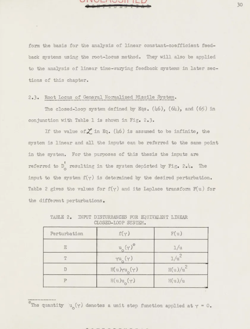
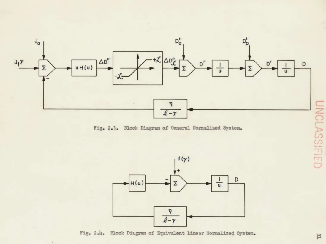
2.3. Root Locus of General Normalized Missile System.

The closed-loop system defined by Eqs. (46), (64), and (65) in conjunction with Table 1 is shown in Fig. 2.3.

If the value ofZ in Eq. (46) is assumed to be infinite, the system is linear and all the inputs can be referred to the same point in the system. For the purposes of this thesis the inputs are

referred to D resulting in the system depicted by Fig. 2.4. The

0

input to the system f(y) is determined by the desired perturbation. Table 2 gives the values for f(y) and its Laplace transform F(u) for the different perturbations.

TABLE 2. INPUT DISTURBANCES FOR EQUIVALENT LINEAR CLOSED-LOOP SYSTEM.

Perturbation f(y) F(u)

E u (Y)" 1/u

T Yu (Y) 1/u2

D H(u)yu (y) H(u)/u2

P H(u)u0(y ) H(u)/u

* I

The quantity u₀ (y) denotes a unit step function applied at y 0.

I

I

D

Fig. 2.3. M.ook Diagram of (9neral Nomaliaed System.

C

p

-D L D

-- H (u) _u

--Eaoek Diagerwn Of Bqciva3Ant LIn ar Normalized System.,

JIY

E UH(U)

UNCLASSW I ED

The quantity u is used to represent the normalized complex fre-quency variable

U = V + jp

as well as the normalized differential operator d/dy.

The transfer operator of the system shown in Fig. 2.4 is

1

D

Substituting Eq. (83) into Eq. (82) and multiplying numerator and denominator by u yields

f Y)u + H(u) .(5

Since w is a linear function of y, a direct application of the Laplace transformation to Eq. (85) results in a first-order linear differential equation involving the transforms of D and f(y) along with the first derivatives with respect to u of these transforms.

The solution of this differential equation is discussed in the next chapter. It is sufficient here to state that except for missile control systems that can be represented as a simple lag or criticaly

UNCLASSiF ED

33

damped quadratic transfer function this approach does not readily yield information about the miss-distance curve.

Consider a closed-loop system whose transfer operator has the same form as that of Eq. (85) with the exception that w is not a func-tion of y. For this condition the Laplace transform of Eq. (85)

results in the transfer function

D 186

F u + H(u)A ₍₈₆₎

where the system gain A is defined as

A- (87)

Emphasis should be placed on the fact that the actual system is time-varying and not constant-coefficient. Nevertheless, here and in what follows the root-locus concept will be used to provide bases that

characterize the system.

It is shown in Appendix E that whenC = O0 if the miss-dis tance curve for a particular f(y) is known, the miss-distance curves for other f(y)'s can be found by considering F(u) in Eq. (86) to be a function of the differential operator d/dQ.

The transfer function of the linear constant-coefficient system,

Eq. (86), is characterized by the roots of its characteristic equation

which exist when

uH" (u) +

A

UNCLASb-IU

The root locus of the system is defined as the solutions of

Eq. (88) as E is varied from minus to plus infinity.

During any one trajectory solution the value of w varies from unity to zero. From Eq. (87) this corresponds to a variation in from 1/1 to infinity. Therefore, for a particoular trajectory solu-tion, Eq. (88) can be represented as the portion of the root locus

that exists for

1:5 A

<

The miss-distance curve is defined as the value of the trajec-tory solution when y = (7. For most systems the miss-distance curves give the most useful information when

05 5 10.

Thus only the part of the root locus where

need be considered.

When n - m for the function uH (u) is greater than two, at least one set of complex branches of the locus will cross over into

the right half plane as

A

The lowest positive value of

A

Ac.

UNCLASSIFIED

will be used to characterize the system shown in Fig. 2.h in a manner analogous to that of using the roots of Eq. (88) to characterize a

constant-coefficient linear system. Therefore any methods devised for the purpose of estimating the miss-distance curves for higher order missile control systems from the miss-distance curves for quadratic missile control systems must be based upon this portion of the root locus which hereon will be referred to as the dominant branch of the root locus. In order to adopt a logical approach to the problem of devising the aforementioned methods, it is first necessary to study the quadratic systems. In the next section the effects of parameter variations upon the miss-distance curves for underdamped quadratic missile control systems are discussed.

2.h. Quadratic Missile Control Systems.

The transfer function for? the undamped quadratic missile control system is

G(s) (89)

- + cos + 1

m2 n

This transfer function has poles located at

s = -rOn l . (90)

Therefore, from Eqs. (32) and (33),

'rN =2 (91)

and

u .O (92)

n

UlnCLA

r7:zD

36

The combination of Eqs. (37), (89), and (92) results in

H(u) 2 (93)

-U- +u + 1

Several examples of nomalized miss-distance curves obtained on the M.I.T. Flight Simulator for quadratic systems with different values of 11 and t when subjected to aiming-error and target-maneuver perturba-tions are given in Figs. 2.5 to 2.8. It should be recalled that these miss-distance curves are the responses at y = I of the system shown in Fig. 2.4 when H(u) is given by Eq. (93) and f(y) is as presented in Table 2.

The assumption of a probability-distribution density for the occurrence of the perturbation within the range 0:5 5 10 permits the calculation of average and nms values of miss distances for this range and thus affords a means of comparison between the different curves.

For this thesis the probability-distribution density of the

occurrence of the perturbation is assumed to be uniform when 05A 5 10. The rms value of the miss-distance curve is, therefore,

rjs 2

(9)

It is shown in the next chapter that for the system depicted in Fig. 2.4 the integral of the miss-distance curve from zero to infinity is zero for 1 > 2 in the case of aiming error and n > 3 for target maneuver. Thus the average values of the miss-distance curves for linear systems do not contain much information.

37

1.5

1.0

3 4 5 6 7 8 9 10 11 12

Fig. 2.. Nonalied _{Miss Dist.no. Caused by Aiming &rcr with Quadratic} Missile Systam when Y.5 1 andn -w

.

PERTURBATION E -H(u).QUADRATIC :1.0,0.75,0.50,0.25 00 A 0 0 -05 -1.0 -15 0 2 rARmir-(QfAA 101.r lamle )

" I -q L-I

'1

1

FD

38

Nomal1iad Miss Distance Caused

Aiming

Duaped Quadratic Missile yratem where - 2, rror , 6, and 5.with Critiealy

I 0 -0.5 -1.0 -L5 0 Fig. 2.6. PERTURBATION E H(u.)=QUADRATIC n_ =

2, 4, 6,

1.0

t

_L)

39

2.4

0 I 2 3 4 5 6 7 8 9 10 II IZ

UNCLi,

_D

Nonuaaiued M1S1 Distan Camed tv Targpt Mem r with Quadrati Missile System _{when t 5 1 and -rn 4.}

I. Q. 5 0 .5 5 -- -0 -4 .0 PERTURBATION T 4 H(u)=QUADRATIC I.OQ75,050,025 51

----

Fig.

2.7,

CONFIDENTIAL ( ECURITY INFORMATION) 2.0 - - -- ,u...'

...

Uk

Norma4mod Miss Distanc

D-g" Quadratio Missile for Target Maneuver with Critioaly_{%rstsm and n} - 3, h, 6, and 8.

CONFIDENTIAL PERTURBATION T -= 3, 4, 6, 8 H(u)=QUADRATIC 0 OA0 .0 m m m m. 0 C -O.5 -1.0 - 1.5 v Jig. 2.8.

UNCLASSIFIED

I.~, 41

Two of the most easily calculable characteristics of the root locus are the values of gain and frequency crossovers. Using the method discussed in Appendix D: when H(u) is given by Eq. (93),

Rp = Ittu 2 IP = U3 + 4u,

Rz

and

IZ = 0. Therefore from Eq. (D-9),

p c =2 (95)

and from Eq. (D-10),

A C 4t. (96)

From Eq. (95) it is seen that due to the method of normalizing with respect to time employed in this analysis, the crossover frequency

is independent of ( when t5i . Therefore, as was suspected, Eq. (95) shows that no information about the miss-distance curve is imparted by merely considering one point on the locus. However, Eq. (96) is

useful for determining the change in the magnitude of the miss-distance curve produced by vaxying H(u) as shown in the following discussion.

The proportionate amount of time that the root locus is located in the right half plane orc can be found from

1 IL >

1-Ac

(97)

cAc

U

NULIA5SI

I-

ILD

-

0

where

A

In order to relate the effect of or to the miss-distance curve

C

for

o0

j5

C

for this range,

-

f'/A~

c10

ca- +(98)

O~A _{n/ d+1Ac}

Thus

c

1\Ac

A graph of or versus Ac/l is presented in Fig. 2.9. Therefore, by plotting DM-rMB versus 0' , the resultant change in the magnitude of the

miss-distance curve caused by varying the amount of time the locus lies in the right half-plane can be determined. An examination of Figs. 2.10a and 2.10b reveals that DM-M is also a function of variables other

than caT; thus, for the quadratic system, either q or t could be used as a parameter in presenting this graph. The author chose rj as the param-eter for the following reason. Although this thesis deals with the linearized missile control system, the actual system contains nonlin-earities, the most important of which is the command limit discussed in Chapter 1. An analysis of the effects of limit level,t , upon the values of miss distance for missile control systems having no time lags

(that is, H(u) = 1) has been performed by Trembath. 4 _{In this analysis}

it is shown that, for a constant value ofr, the miss-distance curve is a function of I. Therefore, if any attempt is to be made to apply the methods for handling miss-distance curves developed in this thesis

U

Q8

0

i

W

2

AC

Fig. 2.9. Average Proportionate Tim that Root Locus is ocated in Ri Half -Plan where 0 1 10 as FULStion ofiL

UN CLAS

6

1ED

0% 0%& " %i II a 'A a

143

UNCLASSIFIED

to nonlinear missile systems, ri should be treated as a distinct param-eter instead of a gain associated with H(u).

A disadvantage of comparing miss-distance curves on the basis of rms values is that the curves must all have the same value of TN

order for the comparison to be meaningful from the standpoint of the unnormalized system.

It is shown by Figs. 2.10a and 2.10b that a linear underdamped quadratic missile control system with a predetermined value of con will give optimum performance in terms of minimum DM M when t and n have values such that:

a)' _ h for aiming-error perturbations b) or : 5 for target-maneuver perturbations

c

In order to discuss further the miss-distance curves given in Figs. 2.5 to 2.8 in terms of the root loci pertaining to the quadratic systems it is necessary to procure more information about these root loci.

Assume for the moment that Eq. (93) is a special case of

H(u) 2 1 (100)

2

u 2 u

where S= 2. The reason for introducing the variable g will be apparent later on.

Let

%P + J*,(li

U N L T M -r A

V r A . TV. I IP

LNLA~i~rin

L

Fig. 2.10a. B 1 Miss Distance Quadratic Missile Indicated.

Caused by Aiming Rrror vs. ( for Syotamu with Y 1 1 and values of q

'UNCLASSIFEL

0.2

0

0

=5

+71=6

=8

"9 4 4.

4-i LD

3

4-5

6

8

I

I

0.2

0.6

0.8

Rom Miss Distance Caused bt Target Mameuver for Quadratic Misile Control Syateu with Y Values of -n Indicated. Fig. 2.10b.

1.0

x

UNCLASSIFIED

46

5

4

E

0.I

01

C

a.

lv

UNCLASSIFIED

II MiT i l

₄₇

and

Hl(X) =

from the method presented in Appendix D the angle condition of the root-locus equation for

XH" 1(x) +

A=

is

2 32 + 4) p + 1. ₍₁₀₃₎

The magnitude criterion is

-A=

Plots of Eqs. (103) and (104) in the X plane, for various values of r, give the root loci with corresponding values of gain of the feedback system shown in Fig. 2.4, when normalized with respect to A/con* set of such curves is presented in Fig. 2.11.

In Sec. 2.3 it was stated that the usable portion of the locus is found from the condition

R < A<00

< --

<

CO

When -i = _{4, as in the case of Figs. 2.5 and 2.7, the above range} becomes

0.2 _{< O}

UU&LA)ZrI

/06/(1.0

/

/

1

,

/

S

/

- I

7

j3

J2

0.5

p

Gain-Calibrated Dominant Root-Loci Branches for ratio Missile Syatmw with Y,

AIAvkfi, PN

itEDdm

1.0

5-jlH

jQ5

0

-1.5

I