Action Recognition by Dense Trajectories

HAL Id: inria-00583818

https://hal.inria.fr/inria-00583818

Submitted on 7 Apr 2011

HAL is a multi-disciplinary open access

archive for the deposit and dissemination of

sci-entific research documents, whether they are

pub-lished or not. The documents may come from

teaching and research institutions in France or

abroad, or from public or private research centers.

L’archive ouverte pluridisciplinaire HAL, est

destinée au dépôt et à la diffusion de documents

scientifiques de niveau recherche, publiés ou non,

émanant des établissements d’enseignement et de

recherche français ou étrangers, des laboratoires

publics ou privés.

Action Recognition by Dense Trajectories

Heng Wang, Alexander Kläser, Cordelia Schmid, Liu Cheng-Lin

To cite this version:

Heng Wang, Alexander Kläser, Cordelia Schmid, Liu Cheng-Lin. Action Recognition by Dense

Tra-jectories. CVPR 2011 - IEEE Conference on Computer Vision & Pattern Recognition, Jun 2011,

Colorado Springs, United States. pp.3169-3176, �10.1109/CVPR.2011.5995407�. �inria-00583818�

Action Recognition by Dense Trajectories

Heng Wang

Alexander Kl¨aser

Cordelia Schmid

Cheng-Lin Liu

†

_{National Laboratory of Pattern Recognition}

_{LEAR, INRIA Grenoble, LJK}

Institute of Automation, Chinese Academy of Sciences

Grenoble, France

{hwang, liucl}@nlpr.ia.ac.cn {Alexander.Klaser, Cordelia.Schmid}@inria.fr

Abstract

Feature trajectories have shown to be efficient for rep-resenting videos. Typically, they are extracted using the KLT tracker or matching SIFT descriptors between frames. However, the quality as well as quantity of these trajecto-ries is often not sufficient. Inspired by the recent success of dense sampling in image classification, we propose an approach to describe videos by dense trajectories. We sam-ple dense points from each frame and track them based on displacement information from a dense optical flow field. Given a state-of-the-art optical flow algorithm, our trajec-tories are robust to fast irregular motions as well as shot boundaries. Additionally, dense trajectories cover the mo-tion informamo-tion in videos well.

We, also, investigate how to design descriptors to encode the trajectory information. We introduce a novel descriptor based on motion boundary histograms, which is robust to camera motion. This descriptor consistently outperforms other state-of-the-art descriptors, in particular in uncon-trolled realistic videos. We evaluate our video description in the context of action classification with a bag-of-features approach. Experimental results show a significant improve-ment over the state of the art on four datasets of varying

difficulty,i.e. KTH, YouTube, Hollywood2 and UCF sports.

1. Introduction

Local features are a popular way for representing videos. They achieve state-of-the-art results for action classification when combined with a bag-of-features representation. Re-cently, interest point detectors and local descriptors have been extended from images to videos. Laptev and Linde-berg [13] introduced space-time interest points by extend-ing the Harris detector. Other interest point detectors in-clude detectors based on Gabor filters [1, 5] or on the de-terminant of the spatio-temporal Hessian matrix [33]. Fea-ture descriptors range from higher order derivatives (local jets), gradient information, optical flow, and brightness in-formation [5, 14, 24] to spatio-temporal extensions of image

KLT Dense trajectories

Figure 1. A comparison of the KLT tracker and dense trajectories. Red dots indicate the point positions in the current frame. Dense trajectories are more robust to irregular abrupt motions, in partic-ular at shot boundaries (second row), and capture more accurately complex motion patterns.

descriptors, such as 3D-SIFT [25], HOG3D [11], extended SURF [33], or Local Trinary Patterns [34].

However, the 2D space domain and 1D time domain in videos have very different characteristics. It is, therefore, intuitive to handle them in a different manner than via in-terest point detection in a joint 3D space. Tracking inin-terest points through video sequences is a straightforward choice. Some recent methods [20, 21, 27] show impressive results for action recognition by leveraging the motion information of trajectories. Messing et al. [21] extracted feature trajecto-ries by tracking Harris3D interest points [13] with the KLT tracker [18]. Trajectories are represented as sequences of log-polar quantized velocities. Matikainen et al. [20] used

Trajectory description

HOG HOF MBH

Dense sampling in each spatial scale

Tracking in each spatial scale separately

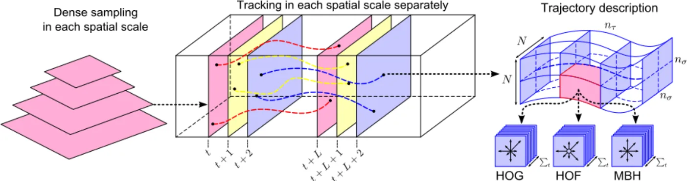
Figure 2. Illustration of our dense trajectory description. Left: Feature points are sampled densely for multiple spatial scales. Middle: Tracking is performed in the corresponding spatial scale over L frames. Right: Trajectory descriptors are based on its shape represented by relative point coordinates as well as appearance and motion information over a local neighborhood of N × N pixels along the trajectory. In order to capture the structure information, the trajectory neighborhood is divided into a spatio-temporal grid of size nσ× nσ× nτ.

a standard KLT tracker. Trajectories in a video are clus-tered, and an affine transformation matrix is computed for each cluster center. The elements of the matrix are used to represent the trajectories. Sun et al. [27] extracted trajecto-ries by matching SIFT descriptors between two consecutive frames. They imposed a unique-match constraint among the descriptors and discarded matches that are too far apart.

Dense sampling has shown to improve results over sparse interest points for image classification [7, 22]. The same has been observed for action recognition in a recent evaluation by Wang et al. [32], where dense sampling at reg-ular positions in space and time outperforms state-of-the-art space-time interest point detectors. In contrast, trajectories are often obtained by the KLT tracker, which is designed to track sparse interest points [18]. Matching dense SIFT de-scriptors is computationally very expensive [15] and, thus, infeasible for large video datasets.

In this paper, we propose an efficient way to extract dense trajectories. The trajectories are obtained by tracking densely sampled points using optical flow fields. The num-ber of tracked points can be scaled up easily, as dense flow fields are already computed. Furthermore, global smooth-ness constraints are imposed among the points in dense opti-cal flow fields, which results in more robust trajectories than tracking or matching points separately, see Figure 1. Dense trajectories have not been employed previously for action recognition. Sundaram et al. [28] accelerated dense trajec-tories computation on a GPU. Brox et al. [2] segmented ob-jects by clustering dense trajectories. A similar approach is used in [17] for video object extraction.

Motion is the most informative cue for action recogni-tion. It can be due to the action of interest, but also be caused by background or the camera motion. This is in-evitable when dealing with realistic actions in uncontrolled settings. How to separate action motion from irrelevant mo-tion is still an open problem. Ikizler-Cinbis et al. [9] applied video stabilization via a motion compensation procedure, where most camera motion is removed. Uemura et al. [30]

segmented feature tracks to separate the motion character-izing the actions from the dominant camera motion.

To overcome the problem of camera motion, we intro-duce a local descriptor that focuses on foreground motion. Our descriptor extends the motion coding scheme based on motion boundaries developed in the context of human detection [4] to dense trajectories. We show that motion boundaries encoded along the trajectories significantly out-perform state-of-the-art descriptors.

This paper is organized as follows. In section 2, we in-troduce the approach for extracting dense trajectories. We, then, show how to encode feature descriptors along the tra-jectories in section 3. Finally, we present the experimental setup and discuss the results in sections 4 and 5 respectively. The code to compute dense trajectories and their description is available online1.

2. Dense trajectories

Dense trajectories are extracted for multiple spatial scales, see Figure 2. Feature points are sampled on a grid spaced by W pixels and tracked in each scale separately. Experimentally, we observed that a sampling step size of W = 5 is dense enough to give good results. We used

8 spatial scales spaced by a factor of 1/√2. Each point

Pt= (xt, yt) at frame t is tracked to the next frame t + 1 by

median filtering in a dense optical flow field ω = (ut, vt).

Pt+1= (xt+1, yt+1) = (xt, yt) + (M ∗ ω)|(¯xt,¯yt), (1)

where M is the median filtering kernel, and (¯xt, ¯yt) is the

rounded position of (xt, yt). This is more robust than

bi-linear interpolation used in [28], especially for points near motion boundaries. Once the dense optical flow field is computed, points can be tracked very densely without ad-ditional cost. Points of subsequent frames are concatenated to form a trajectory: (Pt, Pt+1, Pt+2, . . .). To extract dense

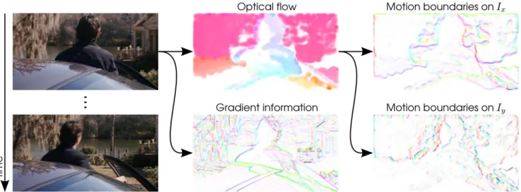
Figure 3. Illustration of the information captured by HOG, HOF, and MBH descriptors. For each image, gradient/flow orientation is indicated by color (hue) and magnitude by saturation. Motion boundaries are computed as gradients of the x and y optical flow components separately. Compared to optical flow, motion boundaries suppress most camera motion in the background and highlight the foreground motion. Unlike gradient information, motion boundaries eliminate most texture information from the static background.

optical flow, we use the algorithm by F¨arneback [6] as im-plemented in the OpenCV library2_{. We found this algorithm}

to be a good compromise between accuracy and speed. A common problem in tracking is drifting. Trajectories tend to drift from their initial location during tracking. To avoid this problem, we limit the length of a trajectory to L frames. As soon as a trajectory exceeds length L, it is re-moved from the tracking process, see Figure 2 (middle). To assure a dense coverage of the video, we verify the presence of a track on our dense grid in every frame. If no tracked point is found in a W × W neighborhood, this feature point is sampled and added to the tracking process. Experimen-tally, we chose a trajectory length of L = 15 frames.

In homogeneous image areas without any structure, it is impossible to track points. Here, we use the same criterion as Shi and Tomasi [26]. When a feature point is sampled, we check the smaller eigenvalue of its autocorrelation ma-trix. If it is below a threshold, this point will not be included in the tracking process. Since for action recognition we are mainly interested in dynamic information, static trajectories are pruned in a pre-processing stage. Trajectories with sud-den large displacements, most likely to be erroneous, are also removed. Figure 1 compares dense and KLT trajecto-ries. We can observe that dense trajectories are more robust and denser than the trajectories obtained by the KLT tracker. The shape of a trajectory encodes local motion patterns. Given a trajectory of length L, we describe its shape by a sequence S = (∆Pt, . . . , ∆Pt+L−1) of displacement

vec-tors ∆Pt = (Pt+1− Pt) = (xt+1− xt, yt+1− yt). The

resulting vector is normalized by the sum of the magnitudes

2_{http://opencv.willowgarage.com/wiki/}

of the displacement vectors:

S0=(∆Pt, . . . , ∆Pt+L−1) Pt+L−1

j=t ||∆Pj||

. (2)

We refer to this vector by trajectory descriptor. We have also evaluated representing trajectories at multiple temporal scales, in order to recognize actions with different speeds. However, this did not improve the results in practice. There-fore, we use trajectories with a fixed length L in our exper-iments.

3. Trajectory-aligned descriptors

Local descriptors computed in a 3D video volume around interest points have become a popular way for video representation [5, 11, 14, 25, 33]. To leverage the motion information in our dense trajectories, we compute descrip-tors within a space-time volume around the trajectory, see Figure 2 (right). The size of the volume is N ×N pixels and L frames. To embed structure information in the represen-tation, the volume is subdivided into a spatio-temporal grid of size nσ× nσ× nτ. The default parameters for our

exper-iments are N = 32, nσ = 2, nτ = 3 , which has shown to

be optimal based on cross validation on the training set of the Hollywood2. We give results using different parameter settings in section 5.3.

Among the existing descriptors for action recognition, HOGHOF [14] has shown to give excellent results on a va-riety of datasets [32]. HOG (histograms of oriented gradi-ents) [3] focuses on static appearance information, whereas HOF (histograms of optical flow) captures the local motion information. We compute HOGHOF along our dense trajec-tories. For both HOG and HOF, orientations are quantized into 8 bins using full orientations, with an additional zero

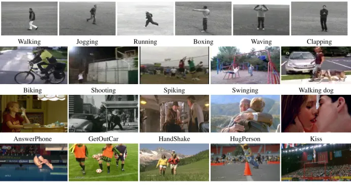
Walking Jogging Running Boxing Waving Clapping

Biking Shooting Spiking Swinging Walking dog

AnswerPhone GetOutCar HandShake HugPerson Kiss

Diving Kicking Walking Skateboarding High-Bar-Swinging

Figure 4. Sample frames from video sequences of KTH (first row), YouTube (second row), Hollywood2 (third row) and UCF sports (last row) action datasets.

bin for HOF (i.e., in total 9 bins). Both descriptors are nor-malized with their L2norm. Figure 3 shows a visualization

of HOGHOF.

Optical flow computes the absolute motion, which in-evitably includes camera motion [9]. Dalal et al. [4] pro-posed the MBH (motion boundary histogram) descriptor for human detection, where derivatives are computed sep-arately for the horizontal and vertical components of the optical flow. This descriptor encodes the relative motion between pixels, as shown in Figure 3. Here we use MBH to describe our dense trajectories.

The MBH descriptor separates the optical flow field Iω = (Ix, Iy) into its x and y component. Spatial

deriva-tives are computed for each of them and orientation infor-mation is quantized into histograms, similarly to the HOG descriptor. We obtain an 8-bin histogram for each

com-ponent, and normalize them separately with the L2 norm.

Since MBH represents the gradient of the optical flow, con-stant motion information is suppressed and only informa-tion about changes in the flow field (i.e., moinforma-tion boundaries) is kept. Compared to video stabilization [9] and motion compensation [30], this is a simple way to eliminate noise due to background motion. This descriptor yields excel-lent results when combined with our dense trajectories. For instance, on the YouTube dataset [16], MBH significantly outperforms HOF, see section 5.

For both HOF and MBH descriptors, we reuse the dense optical flow that is already computed to extract dense tra-jectories. This makes our feature computation process very efficient.

4. Experimental setup

In this section, we first describe the datasets used for action recognition. We, then, briefly present the bag-of-features model used for evaluating our dense trajectory fea-tures as well as the KTL tracking baseline.

4.1. Datasets

Our dense trajectories are extensively evaluated on four standard action datasets: KTH, YouTube, Hollywood2, and

UCF sports, see Figure 4. These datasets are very

di-verse. The KTH dataset views actions in front of a uniform background, whereas the Hollywood2 dataset contains real movies with significant background clutter. The YouTube videos are low quality, whereas UCF sport videos are high resolution.

The KTH dataset [24]3 _{consists of six human action}

classes: walking, jogging, running, boxing, waving and clapping. Each action is performed several times by 25 sub-jects. The sequences were recorded in four different scenar-ios: outdoors, outdoors with scale variation, outdoors with different clothes and indoors. The background is homoge-neous and static in most sequences. In total, the data con-sists of 2391 video samples. We follow the original experi-mental setup of the authors, e.g., divide the samples into test set (9 subjects: 2, 3, 5, 6, 7, 8, 9, 10, and 22) and training set (the remaining 16 subjects). As in the initial paper [24], we train and evaluate a multi-class classifier and report average accuracy over all classes as performance measure.

The YouTube dataset [16]4 contains 11 action cate-gories: basketball shooting, biking/cycling, diving, golf swinging, horse back riding, soccer juggling, swinging, ten-nis swinging, trampoline jumping, volleyball spiking, and walking with a dog. This dataset is challenging due to large variations in camera motion, object appearance and pose, object scale, viewpoint, cluttered background and illumi-nation conditions. The dataset contains a total of 1168 se-quences. We follow the original setup [16] using leave one out cross validation for a pre-defined set of 25 folds. Av-erage accuracy over all classes is reported as performance measure.

The Hollywood2 dataset [19]5 _{has been collected from}

69 different Hollywood movies. There are 12 action classes: answering the phone, driving car, eating, fighting, getting out of car, hand shaking, hugging, kissing, running, sitting down, sitting up, and standing up. In our experiments, we used the clean training dataset. In total, there are 1707 ac-tion samples divided into a training set (823 sequences) and a test set (884 sequences). Train and test sequences come from different movies. The performance is evaluated by computing the average precision (AP) for each of the action classes and reporting the mean AP over all classes (mAP) as in [19].

The UCF sport dataset [23]6 _{contains ten human}

ac-tions: swinging (on the pommel horse and on the floor), diving, kicking (a ball), weight-lifting, horse-riding, run-ning, skateboarding, swinging (at the high bar), golf swing-ing and walkswing-ing. The dataset consists of 150 video samples which show a large intra-class variability. To increase the amount of data samples, we extend the dataset by adding a horizontally flipped version of each sequence to the dataset. Similar to the KTH actions dataset, we train a multi-class classifier and report the average accuracy over all classes. We use a leave-one-out setup and test on each original se-quence while training on all other sese-quences together with their flipped versions (i.e., the flipped version of the tested sequence is removed from the training set).

4.2. Bag of features

To evaluate the performance of our dense trajectories, we use a standard bag-of-features approach. We first construct a codebook for each descriptor (trajectory, HOG, HOF, MBH) separately. We fix the number of visual words per de-scriptor to 4000 which has shown to empirically give good results for a wide range of datasets. To limit the complexity, we cluster a subset of 100,000 randomly selected training features using k-means. To increase precision, we initialize k-means 8 times and keep the result with the lowest error.

4

http://www.cs.ucf.edu/˜liujg/YouTube\_Action\ _dataset.html

5_{http://lear.inrialpes.fr/data}

6_{http://www.cs.ucf.edu/vision/public_html/}

Descriptors are assigned to their closest vocabulary word using Euclidean distance. The resulting histograms of vi-sual word occurrences are used as video descriptors.

For classification we use a non-linear SVM with a χ2

-kernel [14]. Different descriptors are combined in a multi-channel approach as in [31]: K(xi, xj) = exp(− X c 1 AcD(x c i, x c j)), (3)

where D(xci, xcj) is the χ2 distance between video xi and

xj with respect to the c-th channel. Ac is the mean value

of χ2 _{distances between the training samples for the c-th}

channel [36]. In the case of multi-class classification, we use a one-against-rest approach and select the class with the highest score.

4.3. Baseline KLT trajectories

To compare our dense trajectories with the standard KLT tracker [18], we use the implementation of the KLT tracker from OpenCV. In each frame 100 interest points are de-tected, and added to the tracker, which is somewhat denser

than space-time interest points [32]. Interest points are

tracked through the video for L frames. This is identical to the procedure used for our dense trajectories. We also use the same descriptors for the KLT trajectories, e.g. the trajec-tory shape is represented by normalized relative point co-ordinates, and HOG, HOF, MBH descriptors are extracted around the trajectories.

5. Experimental results

In this section, we evaluate the performance of our de-scription and compare to state-of-the-art methods. We also determine the influence of different parameter settings.

5.1. Evaluation of our dense trajectory descriptors

In this section we compare dense and KLT trajectories as well as the different descriptors. We use our default pa-rameters for this comparison. To compute the descriptors,

we set N = 32, nσ= 2, nτ = 3 for both baseline KLT and

dense trajectories. We fix the trajectory length to L = 15, and the dense sampling step size to W = 5.

Results for the four datasets are presented in Table 1. Overall, our dense trajectories outperform the KLT trajec-tories by 2% to 6%. Since the descriptors are identical, this demonstrates that our dense trajectories describe the video structures more accurately.

Trajectory descriptors, which only describe the motion of the trajectories, give surprisingly good results by them-selves, e.g. 90.2% on KTH and 47.7% on Hollywood2 for dense trajectories. This confirms the importance of mo-tion informamo-tion contained in the local trajectory patterns. We report only 67.2% on YouTube because the trajectory

KTH YouTube Hollywood2 UCF sports

KLT Dense trajectories KLT Dense trajectories KLT Dense trajectories KLT Dense trajectories

Trajectory 88.4% 90.2% 58.2% 67.2% 46.2% 47.7% 72.8% 75.2%

HOG 84.0% 86.5% 71.0% 74.5% 41.0% 41.5% 80.2% 83.8%

HOF 92.4% 93.2% 64.1% 72.8% 48.4% 50.8% 72.7% 77.6%

MBH 93.4% 95.0% 72.9% 83.9% 48.6% 54.2% 78.4% 84.8%

Combined 93.4% 94.2% 79.9% 84.2% 54.6% 58.3% 82.1% 88.2%

Table 1. Comparison of KLT and dense trajectories as well as different descriptors on KTH, YouTube, Hollywood2 and UCF sports. We report average accuracy over all classes for KTH, YouTube and UCF sports and mean AP over all classes for Hollywood2.

KTH YouTube Hollywood2 UCF sports

Laptev et al. [14] 91.8% Liu et al. [16] 71.2% Wang et al. [32] 47.7% Wang et al. [32] 85.6%

Yuan et al. [35] 93.3% Ikizler-Cinbis et al. [9] 75.21% Gilbert et al. [8] 50.9% Kovashka et al. [12] 87.27%

Gilbert et al. [8] 94.5% Ullah et al. [31] 53.2% Kl¨aser et al. [10] 86.7%

Kovashka et al. [12] 94.53% Taylor et al. [29] 46.6%

Our method 94.2% Our method 84.2% Our method 58.3% Our method 88.2%

Table 2. Comparison of our dense trajectories characterized by our combined descriptor (Trajectory+HOG+HOF+MBH) with state-of-the-art methods in the literature.

descriptors capture lots of motions from camera. Gener-ally, HOF outperforms HOG as motion is more discrimi-native than static appearance for action recognition. How-ever, HOG gets better results both on YouTube and UCF sports. The HOF descriptors computed on YouTube videos are heavily polluted by camera motions, since many videos are collected by hand-held cameras. Static scene context is very important for UCF sports actions which often involve specific equipment and scene types. MBH consistently out-performs the other descriptors on all four datasets. The im-provement is most significant on the uncontrolled realistic datasets YouTube and Hollywood2. For instance, MBH is 11.1% better than HOF on YouTube. This confirms the ad-vantage of suppressing background motion when dealing with optical flow.

5.2. Comparison to the state of the art

Table 2 compares our results to state of the art. On KTH, we obtain 94.2% which is comparable to the state of the art, i.e., 94.53% [12]. Note that on this dataset several au-thors use a leave-one-out cross-validation setting. Here, we only compare to those using the standard setting [24]. Inter-estingly, MBH alone obtains a slightly better performance on KTH, i.e., 95.0%, than combining all the descriptors together. Ullah et al. [31] also found that a combination of descriptors performed worse than a subset of them. On YouTube, we significantly outperform the current state-of-the-art method [9] by 9%, where video stabilization is used to remove camera motion. We report 58.3% on Hollywood2 which is an improvement of 5% over [31]. Note that Ullah et al. [31] achieved better results by using additional images collected from Internet. The difference between all methods is rather small on UCF sports, which is largely due to the leave-one-out setting, e.g. 149 videos are used for training and only one for testing. Nevertheless, we outperform the state of the art [12] by 1%.

We also compare the results per action class for YouTube

and Hollywood2. On YouTube, our dense trajectories give best results for 8 out of 11 action classes when compare with the KLT baseline and the approach of [9], see Table 3. On Hollywood2, we compare the AP of each action class with the KLT baseline and the approach of [31], i.e., a com-bination of 24 spatio-temporal grids, see Table 4. Our dense trajectories yield best results for 8 out of 12 action classes.

KLT Dense trajectories Ikizler-Cinbis [9]

b shoot 34.0% 43.0% 48.48% bike 87.6% 91.7% 75.17% dive 99.0% 99.0% 95.0% golf 95.0% 97.0% 95.0% h ride 76.0% 85.0% 73.0% s juggle 65.0% 76.0% 53.0% swing 86.0% 88.0% 66.0% t swing 71.0% 71.0% 77.0% t jump 93.0% 94.0% 93.0% v spike 96.0% 95.0% 85.0% walk 76.4% 87.0% 66.67% Accuracy 79.9% 84.2% 75.21%

Table 3. Accuracy per action class for the YouTube dataset. We compare with the results reported in [9].

KLT Dense trajectories Ullah [31]

AnswerPhone 18.3% 32.6% 25.9% DriveCar 88.8% 88.0% 85.9% Eat 73.4% 65.2% 56.4% FightPerson 74.2% 81.4% 74.9% GetOutCar 47.9% 52.7% 44.0% HandShake 18.4% 29.6% 29.7% HugPerson 42.6% 54.2% 46.1% Kiss 65.0% 65.8% 55.0% Run 76.3% 82.1% 69.4% SitDown 59.0% 62.5% 58.9% SitUp 27.7% 20.0% 18.4% StandUp 63.4% 65.2% 57.4% mAP 54.6 58.3% 51.8%

Table 4. Average precision per action class for the Hollywood2 dataset. We compare with the results reported in [31].

5 10 15 20 25 30 35 40 0.5 0.51 0.52 0.53 0.54 0.55 0.56 0.57 0.58 0.59 0.6 Mean Avera ge Precisio n −− Hollyw ood2

Trajectory Length L (frames)

5 10 15 20 25 30 35 400.75 0.76 0.77 0.78 0.79 0.8 0.81 0.82 0.83 0.84 0.85 Average Accuracy −− Y ouTube Hollywood2 YouTube 2 5 8 11 14 17 20 0.54 0.55 0.56 0.57 0.58 0.59 0.6 Mean Avera ge Precisio n −− Hollyw ood2

Sampling Stride W (pixels)

2 5 8 11 14 17 200.79 0.8 0.81 0.82 0.83 0.84 0.85 Average Accuracy −− Y ouTube Hollywood2 YouTube 16 24 32 40 48 56 0.5 0.51 0.52 0.53 0.54 0.55 0.56 0.57 0.58 0.59 0.6 Mean Avera ge Precisio n −− Hollyw ood2

Neighborhood Size N (pixels)

16 24 32 40 48 56 0.75 0.76 0.77 0.78 0.79 0.8 0.81 0.82 0.83 0.84 0.85 Average Accuracy −− Y ouTube Hollywood2 YouTube 1x1x1 1x1x2 1x1x3 2x2x1 2x2x2 2x2x3 3x3x1 3x3x2 3x3x3 0.5 0.51 0.52 0.53 0.54 0.55 0.56 0.57 0.58 0.59 0.6 Mean Avera ge Precisio n −− Hollyw ood2

Cell Grid Structure n_σx n_σx n_τ

1x1x1 1x1x2 1x1x3 2x2x1 2x2x2 2x2x3 3x3x1 3x3x2 3x3x3 0.75 0.76 0.77 0.78 0.79 0.8 0.81 0.82 0.83 0.84 0.85 Average Accuracy −− Y ouTube Hollywood2 YouTube

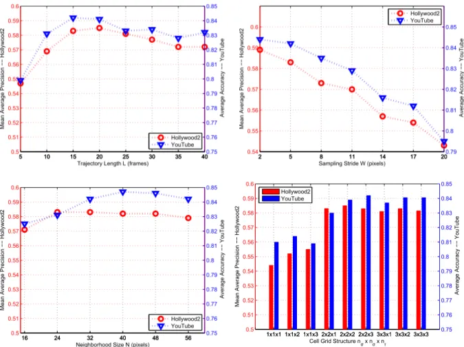
Figure 5. Results for different parameter settings on the Hollywood2 and YouTube datasets.

5.3. Evaluation of trajectory parameters

To evaluate the different parameter settings for dense tra-jectories, we report results on YouTube and Hollywood2, as they are larger and more challenging than the other two. We study the impact of the trajectory length, sampling step size, neighborhood size and cell grid structure. We evaluate the performance for a parameter at the time. The other param-eters are fixed to the default values, i.e., trajectory length L = 15, sampling step size W = 5, neighborhood size N = 32 and cell grid structure nσ= 2, nτ = 3.

Figure 5 (top, left) evaluates the impact of the trajectory length L. For both datasets an increase of length L improves performance up to a certain point (L=15 or 20), and then decreases slightly, since longer trajectories have a higher chance to drift from the initial position. We achieve the best results with a trajectory length of 15 or 20 frames.

With respect to the sampling step size W , Figure 5 (top, right) shows that dense sampling improves the results as the step size decreases. This is consistent with dense sampling at regular positions [32], where more features in general im-prove the results. We report 58.9% (58.3%) on Hollywood2 and 84.4% (84.2%) on YouTube for a step size of 2 (5)

pix-els. A sampling step of 2 pixels is extremely dense, i.e., every other pixel is sampled, and does not justify the minor gain obtained.

The results are relatively stable with regard to the neigh-borhood size N , see Figure 5 (bottom left). On Holly-wood2, results are almost the same when N changes from 24 pixels to 48 pixels. The best result on YouTube is 84.7% with a neighborhood size of 40 pixels. Dividing the video volume into cells improves the results on both Hollywood2 and YouTube. In particular, the performance increases sig-nificantly when the spatial cell grid nσis increased from 1

to 2, see Figure 5 (bottom right). However, further increas-ing the number of cells, i.e., beyond nσ = 2, nτ = 3, does

not improve the results.

6. Conclusions

This paper has introduced an approach to model videos by combining dense sampling with feature tracking. Our dense trajectories are more robust than previous video

de-scriptions. They capture the motion information in the

videos efficiently and show improved performance over

have also introduced an efficient solution to remove camera motion by computing motion boundaries descriptors along the dense trajectories. This successfully segments the rele-vant motion from background motion, and outperforms pre-vious video stabilization methods. Our descriptors combine trajectory shape, appearance, and motion information. Such a representation has shown to be efficient for action classifi-cation, but could also be used in other areas, such as action localization and video retrieval.

Acknowledgments. This work was partly supported by Na-tional Natural Science Foundation of China (NSFC) under grant no.60825301 as well as the joint Microsoft/INRIA project and the European integrated project AXES.

References

[1] M. Bregonzio, S. Gong, and T. Xiang. Recognising action as clouds of space-time interest points. In CVPR, 2009. [2] T. Brox and J. Malik. Object segmentation by long term

analysis of point trajectories. In ECCV, 2010.

[3] N. Dalal and B. Triggs. Histograms of oriented gradients for human detection. In CVPR, 2005.

[4] N. Dalal, B. Triggs, and C. Schmid. Human detection using oriented histograms of flow and appearance. In ECCV, 2006. [5] P. Doll´ar, V. Rabaud, G. Cottrell, and S. Belongie. Behavior recognition via sparse spatio-temporal features. In VS-PETS, 2005.

[6] G. Farneb¨ack. Two-frame motion estimation based on poly-nomial expansion. In Scandinavian Conference on Image Analysis, 2003.

[7] L. Fei-Fei and P. Perona. A Bayesian hierarchical model for learning natural scene categories. In CVPR, 2005.

[8] A. Gilbert, J. Illingworth, and R.Bowden. Action recognition using mined hierarchical compound features. IEEE PAMI, 2011.

[9] N. Ikizler-Cinbis and S. Sclaroff. Object, scene and actions: Combining multiple features for human action recognition. In ECCV, 2010.

[10] A. Kl¨aser, M. Marszałek, I. Laptev, and C. Schmid. Will person detection help bag-of-features action recognition? In Technical Report, INRIA Grenoble - Rhone-Alpes, 2010. [11] A. Kl¨aser, M. Marszałek, and C. Schmid. A spatio-temporal

descriptor based on 3D-gradients. In BMVC, 2008. [12] A. Kovashka and K. Grauman. Learning a hierarchy of

dis-criminative space-time neighborhood features for human ac-tion recogniac-tion. In CVPR, 2010.

[13] I. Laptev and T. Lindeberg. Space-time interest points. In ICCV, 2003.

[14] I. Laptev, M. Marszałek, C. Schmid, and B. Rozenfeld. Learning realistic human actions from movies. In CVPR, 2008.

[15] C. Liu, J. Yuen, and A. Torralba. Nonparametric scene pars-ing: label transfer via dense scene alignment. In CVPR, 2009.

[16] J. Liu, J. Luo, and M. Shah. Recognizing realistic actions from videos in the wild. In CVPR, 2009.

[17] W.-C. Lu, Y.-C. F. Wang, and C.-S. Chen. Learning dense optical-flow trajectory patterns for video object extraction. In IEEE Conference on Advanced Video and Signal Based Surveillance, 2010.

[18] B. D. Lucas and T. Kanade. An iterative image registration technique with an application to stereo vision. In Interna-tional Joint Conference on Artificial Intelligence, 1981. [19] M. Marszałek, I. Laptev, and C. Schmid. Actions in context.

In CVPR, 2009.

[20] P. Matikainen, M. Hebert, and R. Sukthankar. Trajectons: Action recognition through the motion analysis of tracked features. In ICCV workshop on Video-oriented Object and Event Classification, 2009.

[21] R. Messing, C. Pal, and H. Kautz. Activity recognition using the velocity histories of tracked keypoints. In ICCV, 2009. [22] E. Nowak, F. Jurie, and B. Triggs. Sampling strategies for

bag-of-features image classification. In ECCV, 2006. [23] M. Rodriguez, J. Ahmed, and M. Shah. Action MACH: A

spatio-temporal maximum average correlation height filter for action recognition. In CVPR, 2008.

[24] C. Sch¨uldt, I. Laptev, and B. Caputo. Recognizing human actions: A local SVM approach. In ICPR, 2004.

[25] P. Scovanner, S. Ali, and M. Shah. A 3-dimensional SIFT descriptor and its application to action recognition. In ACM Multimedia, 2007.

[26] J. Shi and C. Tomasi. Good features to track. In CVPR, 1994. [27] J. Sun, X. Wu, S. Yan, L.-F. Cheong, T.-S. Chua, and J. Li. Hierarchical spatio-temporal context modeling for ac-tion recogniac-tion. In CVPR, 2009.

[28] N. Sundaram, T. Brox, and K. Keutzer. Dense point trajecto-ries by GPU-accelerated large displacement optical flow. In ECCV, 2010.

[29] G. W. Taylor, R. Fergus, Y. LeCun, and C. Bregler. Convolu-tional learning of spatio-temporal features. In ECCV, 2010. [30] H. Uemura, S. Ishikawa, and K. Mikolajczyk. Feature

track-ing and motion compensation for action recognition. In BMVC, 2008.

[31] M. M. Ullah, S. N. Parizi, and I. Laptev. Improving bag-of-features action recognition with non-local cues. In BMVC, 2010.

[32] H. Wang, M. M. Ullah, A. Kl¨aser, I. Laptev, and C. Schmid. Evaluation of local spatio-temporal features for action recog-nition. In BMVC, 2009.

[33] G. Willems, T. Tuytelaars, and L. V. Gool. An efficient dense and scale-invariant spatio-temporal interest point detector. In ECCV, 2008.

[34] L. Yeffet and L. Wolf. Local trinary patterns for human ac-tion recogniac-tion. In ICCV, 2009.

[35] J. Yuan, Z. Liu, and Y. Wu. Discriminative subvolume search for efficient action detection. In CVPR, 2009.

[36] J. Zhang, M. Marszałek, S. Lazebnik, and C. Schmid. Local features and kernels for classification of texture and object categories: A comprehensive study. IJCV, 73(2):213–238, 2007.