HAL Id: hal-01066076
https://hal.inria.fr/hal-01066076
Submitted on 19 Sep 2014
HAL is a multi-disciplinary open access
archive for the deposit and dissemination of
sci-entific research documents, whether they are
pub-lished or not. The documents may come from
teaching and research institutions in France or
abroad, or from public or private research centers.
L’archive ouverte pluridisciplinaire HAL, est
destinée au dépôt et à la diffusion de documents
scientifiques de niveau recherche, publiés ou non,
émanant des établissements d’enseignement et de
recherche français ou étrangers, des laboratoires
publics ou privés.
Layer Decomposition: An Effective Structure-based
Approach for Scientific Workflow Similarity
Johannes Starlinger, Sarah Cohen-Boulakia, Sanjeev Khanna, Susan
Davidson, Ulf Leser
To cite this version:
Johannes Starlinger, Sarah Cohen-Boulakia, Sanjeev Khanna, Susan Davidson, Ulf Leser. Layer
De-composition: An Effective Structure-based Approach for Scientific Workflow Similarity. International
Conference on e-Science, Oct 2014, Guarujá, Brazil. pp.169-176, �10.1109/eScience.2014.19�.
�hal-01066076�
Layer Decomposition: An Effective Structure-based
Approach for Scientific Workflow Similarity
Johannes Starlinger
∗, Sarah Cohen-Boulakia
†, Sanjeev Khanna
‡, Susan B. Davidson
‡, and Ulf Leser
∗∗Humboldt Universit¨at zu Berlin †Universit´e Paris-Sud ‡University of Pennsylvania
Institut f¨ur Informatik Laboratoire de Dep. of Computer and Information Science Unter den Linden 6, Recherche en Informatique 3330 Walnut Street
10099 Berlin, Germany CNRS UMR 8623, France Philadelphia, PA 19104-6389, USA {starling, leser}@informatik.hu-berlin.de INRIA, LIRMM, IBC {sanjeev, susan}@cis.penn.edu
Abstract—Scientific workflows have become a valuable tool for large-scale data processing and analysis. This has led to the creation of specialized online repositories to facilitate workflow sharing and reuse. Over time, these repositories have grown to sizes that call for advanced methods to support workflow discovery, in particular for effective similarity search. Here, we present a novel and intuitive workflow similarity measure that is based on layer decomposition. Layer decomposition accounts for the directed dataflow underlying scientific workflows, a property which has not been adequately considered in previous methods. We comparatively evaluate our algorithm using a gold standard for 24 query workflows from a repository of almost 1500 scientific workflows, and show that it a) delivers the best results for similarity search, b) has a much lower runtime than other, often highly complex competitors in structure-aware workflow comparison, and c) can be stacked easily with even faster, structure-agnostic approaches to further reduce runtime while retaining result quality.
I. INTRODUCTION
Scientific workflow systems have become an established tool for creating and running reproducible in-silico experi-ments. With their increasing popularity, online repositories of scientific workflows have emerged as a means of facilitating sharing, reuse, and repurposing. Examples of such repositories include CrowdLabs [1], SHIWA [2], and the Galaxy repository [3]. Probably the largest workflow collection is myExperiment [4], which currently contains more than 2500 workflows from various disciplines, including bioinformatics, astrophysics, and earth sciences. To make the best use of these repositories, users need support to find workflows that match their specific needs [5]. However, currently these repositories only support key-word queries which are matched against textual descriptions, tags, and titles given to the workflows upon upload [2], [3], [1], [4]. Obviously, the quality of such a search critically depends on the quality of the annotations associated with workflows.
Scientific workflows typically resemble directed acyclic graphs (DAGs) consisting of global input and output ports, data processing modules, and datalinks which define the flow of data from one module to the next. Two sample workflows from myExperiment are shown in Figure 1. Therefore, another source of information that can be exploited for search is the structure or topology of the workflow [6]. An obvious advantage of structure-based approaches to workflow similarity search is that they do not require any additional information
to be provided by the workflow designer apart from the workflow itself. Structure-based approaches are typically used in a second search phase: First, users identify workflows which roughly match their needs using keyword search. In the second phase, users select one candidate workflow and let the system retrieve functionally similar workflows, i.e., the system performs a workflow similarity search.
Several studies have investigated different techniques for assessing workflow similarity using this structure [7], [8], [6], [9], [10], [11], [12], but initial results indicate that they perform no better, and sometimes even worse, than annotation-based methods in terms of retrieval quality [13], [8], [11]. However, these comparisons were performed on very small and well-documented workflow sets, and thus the results should not be extrapolated to the large, but shallowly annotated repositories that exist today. To verify this hypothesis, in prior work we performed a large-scale comparative evaluation of workflow similarity search algorithms [14]. Our results indicated that a) structure-based methods are indispensable for some current repositories which lack rich annotations, b) structure-based methods, once properly configured, outperform annotation-based methods even when such rich annotations are available, and c) any such standalone approach is further beaten by ensembles of annotation-based and structure-based methods. We also discovered that both the amount of configuration required and runtime considerations were drawbacks to such methods: Fast workflow comparison using annotations on the workflows’ modules provides best results only when ubiqui-tous, functionally unspecific modules are removed from the workflows in a preprocessing step. The configuration of which modules are to be removed is specific to a given dataset, and is non-trivial. Methods based on workflow substructures, on the other hand, provide rather stable results across different configurations, but have prohibitive runtimes.
In this paper, we present a novel technique for measuring workflow similarity that accounts for the directed dataflow underlying scientific workflows. The central idea is the deriva-tion of a Layer Decomposideriva-tion for each workflow, which is a compact, ordered representation of its modules, suitable for effective and efficient workflow comparison. We show that the algorithm a) delivers the best results in terms of retrieval quality when used stand-alone, b) is faster than other algorithms that account for the workflows’ structure, and c) can be combined with other measures to yield better retrieval
Fig. 1: Sample scientific workflows from the myExperiment repository: (a) ID: 1189, Title: KEGG pathway analysis, (b) ID: 2805, Title: Get Pathway-Genes by Entrez gene id.
at even higher speed. Furthermore, the method is essentially configuration free, which makes it applicable off-the-shelf to any workflow repository.
In the remainder of this paper, we first review related work on similarity measures for scientific workflows in Section II. In Section III, we briefly summarize results from [14]. Section IV introduces our Layer Decomposition algorithm for scientific workflow comparison, which we comparatively evaluate in Section V. We conclude in Section VI.
II. RELATEDWORK
Existing approaches to the assessment of scientific work-flow similarity are either based on the associated annotations or on the structure of the workflows themselves. We here name a number of prominent approaches in increasing order of using topological information; for a more detailed comparison see [14]. Using only workflow annotations, Costa et al. [13] derived bags of words from the descriptions of workflows to determine workflow similarity. Keyword tags assigned to workflows are explored by Stoyanovich et al. [11]. The sets of
modulescontained in workflows have been used by Silva et al.
[10], Santos et al. [9], and Friesen et al. [8]. Bergman et al. [7] extended this idea by additionally comparing the workflows’ datalinks based on semantic annotations; however, such seman-tic annotations are not generally available in publicly available workflow repositories. Considering workflow substructure, the use of Maximum Common Isomorphic Subgraphs (MCS) has been investigated by Goderis et al. [6], Santos et al. [9], and Friesen et al. [8]: the latter also proposed using Graph Kernels derived from frequent subgraphs in a repository. Subgraph comparison has also been applied in similar domains, e.g., by Corrales et al. [15] to compare BPEL workflows or by Krinke [16] to compare program dependence graphs. Finally, using the full graph structure, Xiang et al. [12] compute scientific workflow similarity from their Graph Edit Distance.
Note that workflow provenance or semantic annotations could also be taken into account; however, we are not aware of any such data being available within current public
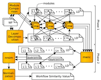
repos-Fig. 2: Workflow comparison process, see also [14]
itories, and therefore do not consider these methods in this paper.
III. PRELIMINARIES
In [14], we report on a comprehensive evaluation of pre-vious approaches to workflow similarity search. In addition to comparing retrieval quality quantitatively, we also introduce a framework (shown in Figure 2) for qualitatively comparing different systems. This is an important tool, as the process of workflow comparison entails many steps, of which a con-crete topology-comparison algorithm is just one. First, the similarity of each pair of modules from two workflows is determined using pairwise module comparison. Second, using these pairwise module similarities, a mapping of modules onto each other is established. This mapping may be influenced by the topological decomposition of the workflows imposed by the third step of topological comparison, which in turn uses the established mapping to assess the similarity of the two workflows. Finally, normalization of the derived similar-ity value wrt the sizes of the compared workflows may be desirable. This process of scientific workflow comparison is preceded by an (optional) additional preprocessing step. Such preprocessing may, for instance, alter the workflows’ structure based on externally supplied knowledge about the elements it contains (see Section III-D).
As each of these steps has a notable impact on the concrete values computed and thus the assessment of different algorithms, we describe them in more detail in the following. Note that our novel Layer Decomposition method (described in the next section) is a contribution dedicated to the step of
topological decomposition and comparison; in Section V, we
will compare different approaches to this step while keeping all other steps constant.
A. Module Comparison
Structure-based approaches to workflow similarity perform some type of comparison of the two workflow graphs. To this end, they must be able to measure the similarity of two nodes in the graphs, which represent two modules in the to-be-compared workflows. Module comparison is typically approached by comparing the values of their attributes. These range from identifiers for the type of operation to be carried out, to the descriptive label of the module given to it by the workflow’s author, to rather specific attributes such as the
url of a web-service to be invoked. In [14] we compared
and showed that choosing a suitable configuration is most crucial for result quality of structural workflow comparison. Here, we will use the following three schemes to test the impact of module comparison on the topological comparison provided by our new algorithm:
• pw0 assigns uniform weights to all attributes and com-pares module type, and the web-service related properties
au-thority name, service name, and service uri using exact string
matching. Module labels, descriptions, and scripts in scripted modules are compared using Levenshtein edit distance.
• pw3 compares single attributes in the same way as pw0 but uses higher weights for labels, script and service uri, followed by service name and service authority in the order listed. This weighting resembles the proposal of [10].
• pll disregards all attributes but the labels and compares them using the Levenshtein edit distance, which is the ap-proach taken in [7].
B. Module Mapping
Structural comparison of two graphs may be carried out by comparing all nodes of one graph to all nodes of the other graph, or by first computing a node mapping which defines the set of allowed node associations (often one-to-one). Only then do graph operations such as node deletion or node insertion make sense. In [14] we compared different strategies to obtain such a mapping; in this work, we use two strategies, depending on the amount of topological information available:
• maximum weight matching (mw) chooses the set of one-to-one mappings that maximizes the sum of similarity values for unorderes sets of nodes.
• maximum weight non-crossing matching (mwnc) [17] requires an order on each of the two sets to be mapped to be given by the graphs’ topological decompositions. Given two ordered lists of modules(m1, ..mi, ..mk) and (m′1, ..m′j, ..m′l),
a mapping of maximum weight between the sets is computed with the additional constraints no pair of mappings (mi, m′j)
and(mi+x, m′j−y) may exist with x, y ≥ 1. C. Normalization
A difficult problem in topological comparison of workflows is how to deal with differences in workflow size. In particular, given a pair V , W of workflows where V ⊂ W and |W | >> |V |, what is their similarity? This decision typically is encoded in a normalization of similarity values wrt the sizes of the two workflows [14]. In this work, we use a variation of the Jaccard similarity coefficient, which measures the similarity of two sets A and B by their relative overlap: |A|+|B|−|A∩B||A∩B| . We modify this formula because the methods for comparing modules do not create binary decisions but instead return a similarity score; details can be found in [14].
D. External Knowledge
When comparing two workflows, knowledge derived from the entire workflow repository or even from external sources may be taken into account. While this idea in theory could be implemented by complex inferencing processes over process ontologies and formal semantic annotations, our results in
[14] showed that the following two simple and efficiently computable options are already quite effective:
• Importance Projection Preprocessing. Many modules in real-world workflows actually convey little information about workflow function, but only provide parameter settings, perform simple format conversions, or unnest structured data objects [18]. Importance projection is the process of remov-ing such modules from a workflow prior to its comparison, where the connectivity of the graph structure is retained by transitive reduction of removed paths between the remaining modules. Note that this method requires external knowledge given in the form of a method to assess the contribution of a given module to the workflow’s function, which is a rather strong requirement. The implementation provided here relies on manual assignments of importance based on the type of operation carried out by a given module.
• Module Pair Preselection. Instead of computing all pairwise module similarities for two workflows prior to further topological comparisons, this method first classifies modules by their type and then compares modules within the same class. This reduces the number of (costly) module comparisons and may even improve mapping quality due to the removal of false mappings across types. Here, external knowledge must be given in the form of a method assigning a predefined class to each module.
IV. LAYERDECOMPOSITIONWORKFLOWSIMILARITY
In this section, we present a novel approach, called Layer
Decomposition (LD), for structurally comparing two
work-flows. The fundamental idea behind LD is to focus on the order in which modules are executed in both workflows by only permitting mappings of modules to be used for similarity assessment which respect this order (in a sense to be explained below). Two observations led us to consider execution order as a fundamental ingredient to workflow similarity. First, it is intuitive: The function of a workflow obviously critically depends on the execution order of its tasks as determined by the direction of data links; even two workflows consisting of exactly the same modules might compute very different things if these modules are executed in a different order. Nevertheless, most structural comparison methods downplay execution order. For instance, it is completely lost when only module sets are compared, and a few graph edits can lead to workflows with very different execution orders (like swapping the first and last of a long sequence of modules). Second, we observed in our previous evaluation [14] that approaches to topological workflow comparison which put some focus on execution order are much more stable across different configurations of the remaining steps of the workflow comparison process. In particular, comparing two graphs using their path sets, i.e., the set of all paths from a source to a sink, produced remarkably stable results both with and without the use of external knowledge. Inclusion of such knowledge in workflow comparison had among the largest impact on the overall performance of methods, but requires corpus-specific expert intervention. Based on these findings, developing methods that achieve retrieval results of high quality without requiring external knowledge seemed like a promising next step.
In the following, we first explain how LD extracts an or-dering of workflow modules from the workflow DAG. We then
Fig. 3: Sample layer decomposition and layer mapping of scientific workflows (a) 1189, (b) 2805; see also Fig. 1).
show in Section IV-B how two workflows can be effectively compared using this partial ordering. Finally, we explain in Section IV-C how normalization is performed.
A. Topological Decomposition
The linearization (or topological sort) of a DAG is an ordering of its nodes V such that node u precedes node v in the ordering, if an edge (u, v) exists. Obviously, a DAGs linearization can be computed in linear time using topological sorting; however, it is generally not unique. As the quality of the subsequent mapping (see below) depends on the concrete linearizations chosen for the two workflows under consider-ation, it is important to find a good pair of linearizations, i.e., linearizations such that highly similar modules will later get mapped onto each other. Since the number of possible linearizations isΩ(n!) (where n is the number of modules in a workflow), assessing all possible pairs is generally infeasible; it is also infeasible in practice, as many real life workflows have many different linearizations (for instance, 23.5% of the 1485 Taverna workflows in our evaluation set have more than 100 different linearizations).
We tackle this problem by representing all possible lin-earizations of a given workflow in a concise data structure. Observe that a DAG has more than one linearization iff between two consecutive nodes in one of its linearizations no direct datalink exists, because in this case swapping the two nodes creates another linearization. In all such cases, we tie the two nodes in question into a single position in the ordering. We call such a tie at position i a layer Li. Compacting all
sequences of two or more swappable nodes of a linearization in this way yields a layered ordering of the DAG which we call its layer decomposition LD = (L1, .., Li, .., Lk). Note
that the layer decomposition of a DAG is unique, as a) layers themselves are orderless sets of modules, and b) following from the definition of the underlying linearization, for any Li and Lj such that i < j, for every v ∈ Lj, there is
some u ∈ Li which precedes v in every linearization, which
c) uniquely defines the positions of Li and Lj within the
decomposition. To compute a workflow’s layer decomposition, we use a simple iterative algorithm. First, all modules with in-degree 0 (the DAGs source nodes) form the top layer L1. These
modules and all their outbound data links are removed from the workflow; this process is repeated until no more modules remain. Figure 3 shows the layer decompositions of the sample workflows introduced in Figure 1. In the figure, the different
Fig. 4: Overview of workflow comparison applied by LD
layers are visually aligned to reflect their mapping, as it is derived in the following step.
B. Topological Comparison
The layer decomposition of a workflow partitions its mod-ule set by execution order creating an ordered list of modmod-ule subsets. To compare the layer decompositions LD and LD′of two workflows wf and wf′, respectively, we take a two-phase approach, sketched in Figure 4. First, pairwise similarity scores for each pair of layers (L, L′) ∈ LD × LD′ are computed
from the modules they contain using the maximum weight matching (mw), based on the similarity values p(m, m′)
derived by a given module comparison scheme as introduced in Section III-B:
layersim(L, L′) =Xp(m, m′) | (m, m′) ∈ mw(L, L′) In the second phase, the ordering of the layers - and thus of the modules they are comprised of - is exploited to compute the decompositions’ maximum weight non-crossing matching (mwnc) with the pairwise similarities of layers from phase one. The resulting layer-mapping serves as the basis for the overall (yet non-normalized) similarity score of the compared workflows using LD:
nnsimLD(wf, wf′) =
X
layersim(L, L′) | (L, L′) ∈ mwnc(LD, LD′)
C. Normalization
As done for all other methods we shall compare to, we normalize the similarity values computed by LD using the Jaccard variation described in Section III-C. Thus, the final, normalized LD-similarity is computed as:
simLD(wf, wf′) =
nnsimLD
|LD| + |LD′| − nnsim LD
. We analogously normalize layersim(L, L′) by |L| and |L′|.
This way, if two workflows are identical, each layer has a mapping with a similarity value of 1. Then nnsimLD =
|mwnc(LD, LD′)| = |LD| = |LD′|, and sim
TABLE I: Algorithm shorthand notation overview
Notation Description
Algorithms
LD Layer Decompositiontopological comparison MS Module Setstopological comparison PS Path Setstopological comparison GE Graph Edit Distancetopological comparison BW Bag of Wordsannotation based comparison
BT Bag of Tagsannotation based comparison
Configurations
np No structural preprocessing of workflows
ip Importance projectionworkflow preprocessing
ta No module pair preselection for comparison
te Type equivalencebased module pair preselection
pw0 Module comparison with uniform attribute weights
pw3 Module comparison on tuned attribute weights
pll Module comparison by edit distance of labels only
V. EVALUATION
We evaluate our novel Layer Decomposition algorithm on a gold standard corpus of workflow similarity ratings given by workflow experts. We therein use the data and setup from [14]1. The corpus contains 2424 similarity ratings from 15
experts from four countries for 485 workflow pairs from a set of 1485 Taverna workflows, given along a four step Likert scale [19] with the options very similar, similar, related, and
dissimilar plus an additional option unsure. The ratings are
grouped by 24 query workflows. Each query workflow has a list of 10 workflows compared to it, which are ranked by a consensus computed from the experts rankings using BioCon-sert Median Ranking [20]. These rankings are used to evaluate the algorithms performance in workflow ranking. For 8 of the query workflows, additional expert ratings are available covering all workflows which were ranked among the top-10 most similar workflows by a selection of algorithms to be further evaluated, when run against the entire workflow corpus. These are used to assess workflow retrieval performance.
Using this corpus, we compare the LD algorithm against approaches based on Module Sets, Path Sets, Graph Edit Distance, Bags of Words, and Bags of Tags (as presented in Section II). First, we investigate the algorithms’ performance in the tasks of workflow ranking (Section V-A) and workflow retrieval (V-B). Second, we compare the runtimes of the differ-ent topological comparison methods (V-C). Third, we evaluate whether the successive application of multiple algorithms in retrieval can improve result quality and its implications on runtime (V-D). Finally, in Section V-E we shall confirm the previous results on ranking performance using a second data set, from the Galaxy repository.
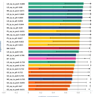
A. Workflow Ranking
To evaluate ranking performance, we use the measures of ranking correctness and completeness [7], [21]. For ranking correctness, the order of each pair of elements in the experts’ consensus ranking and the algorithmic ranking is compared, counting pairs sharing the same order and pairs that don’t, to determine the correlation of the compared rankings. Values range from -1 to 1, where 1 indicates full correlation of the rankings, 0 indicates that there is no correlation, and negative values are given to negatively correlated rankings. Ranking
1All ratings and workflows are available at
https://www.informatik.hu-berlin.de/forschung/gebiete/wbi/resources/flowalike. al go ri th m s ranking correctness
User: BioConsert5, Workflow: mean
-0.4 -0.2 0 0.2 0.4 0.6 0.8 1 GE_np_ta_pw0: 0.631 GE_np_ta_pll: 0.67 GE_np_ta_pw3: 0.693 MS_np_ta_pw0: 0.705 GE_ip_te_pw0: 0.705 GE_ip_te_pll: 0.722 GE_ip_te_pw3: 0.732 PS_np_ta_pw0: 0.744 LD_np_ta_pw0: 0.759 BT: 0.765 MS_ip_te_pw0: 0.766 LD_ip_te_pw0: 0.81 BW: 0.819 PS_np_ta_pll: 0.821 PS_ip_te_pw0: 0.822 PS_ip_te_pll: 0.827 MS_np_ta_pw3: 0.829 PS_np_ta_pw3: 0.835 MS_np_ta_pll: 0.84 PS_ip_te_pw3: 0.844 LD_ip_te_pll: 0.856 MS_ip_te_pll: 0.869 LD_ip_te_pw3: 0.869 MS_ip_te_pw3: 0.871 LD_np_ta_pll: 0.88 LD_np_ta_pw3: 0.889
Fig. 5: Mean ranking correctness (bars) with upper and lower stddev (errorbars), and mean ranking completeness (black squares) over 24 lists of 10 workflows for different algorithms and configurations (see Table I for notation).
al go ri th m s ranking correctness
User: BioConsert5, Workflow: mean
-0.4 -0.2 0 0.2 0.4 0.6 0.8 1 ensmbl(BW,GE): 0.703 ensmbl(BW,PS): 0.885 ensmbl(BW,MS): 0.629 ensmbl(BW,LD): 0.914 (a) al go ri th m s ranking correctness
User: BioConsert5, Workflow: mean
-0.4 -0.2 0 0.2 0.4 0.6 0.8 1 ensmbl(BW,GE): 0.742 ensmbl(BW,PS): 0.923 ensmbl(BW,MS): 0.906 ensmbl(BW,LD): 0.934 (b)
Fig. 6: Mean ranking results for ensembles of BW and struc-tural algorithms (a) without and (b) with ip and te, each using pll module comparison.
completeness, on the other hand, measures the number of pairs of ranked elements that are not tied in the expert ranking, but tied in the evaluated algorithmic ranking. The objective here is to penalize the tying of elements by the algorithm when the user distinguishes their ranking position.
Figure 5 shows ranking performance for simLD in direct
comparison to simM S, simP S, simGE, and the annotation
based measures simBW and simBT. Results are sorted by
mean ranking correctness. Each algorithm is applied in a variety of different configurations (see Sections III-A and D for options; see Table I for notation overview). Regarding ranking
k pr ec is io n
User: median, Workflow: mean, Relevance: >=related
MS_ip_te_pll LD_ip_te_pll PS_ip_te_pll MS_np_ta_pll LD_np_ta_pll PS_np_ta_pll _____________ 1 2 3 4 5 6 7 8 9 10 0 0.2 0.4 0.6 0.8 1 (a) k pr ec is io n
User: median, Workflow: mean, Relevance: >=similar
MS_ip_te_pll LD_ip_te_pll PS_ip_te_pll MS_np_ta_pll LD_np_ta_pll PS_np_ta_pll _____________ 1 2 3 4 5 6 7 8 9 10 0 0.2 0.4 0.6 0.8 1 (b)
Fig. 7: Mean retrieval precision at k against the median expert rating for structural similarity algorithms for relevance threshold (a) related, and (b) similar. Algorithms used with module similarity by edit distance of labels (pll), with and without ip and te.
k pr ec is io n
User: median, Workflow: mean, Relevance: >=related
LDpml25_np_ta_pll LD_np_ta_pll MS_np_ta_pll _____________ 1 2 3 4 5 6 7 8 9 10 0 0.2 0.4 0.6 0.8 1 (a) k pr ec is io n
User: median, Workflow: mean, Relevance: >=similar
LDpml25_np_ta_pll LD_np_ta_pll MS_np_ta_pll _____________ 1 2 3 4 5 6 7 8 9 10 0 0.2 0.4 0.6 0.8 1 (b)
Fig. 8: Mean retrieval precision at k for similarity algorithms MS and LD and refined LD penalizing mismatched layers exceeding 25% of the larger workflows layers (LDpml25) for relevance thresholds by median expert rating of (a) related, and (b) similar.
correctness, several observations can be made: Firstly, simLD
provides best results. Secondly, both simLD and simP S
provide most stable results across different configurations. Performance of simM S, on the other hand, varies with the
quality of the module comparison scheme used, and especially with the use of external knowledge in terms of ip. Thirdly, while simM S, when configured properly, can achieve ranking
correctness values comparable to the best results of simLD,
simP Sis generally slighly behind simLD. In contrast, simGE,
putting a high emphasis on overall workflow structure, does not provide competitive results; we therefore omit it in all further evaluations. As for ranking completeness, we see that both simLD and simP S fully distinguish all workflows in terms
of their similarity to the query workflows where users make a distinction as well. The ranking provided by simM S, on the
other hand, is often only near-complete.
Figure 6 shows the results of selected ensembles of dif-ferent base methods using mean similarity values. Generally, result quality improves considerably. For instance, the top performing standalone configuration of simLD achieves a
ranking correctness of 0.889, and is not only outperformed by its combination with simBW by 2.5 %-points, but especially in
terms of stability of results across different query workflows, as apparent from the standard deviations from the mean. The ensembles including simLD deliver better results than other
ensembles especially when no external knowledge is used.
B. Workflow Retrieval
Figure 7 shows mean precision at k [22] for each position in the top-10 results returned by each of the algorithms. We focus our presentation on configurations using the pll module comparison scheme. Comparing simM S, simLD, and simP S,
Figure 7a shows that when treating results as relevant with a median expert rating of at least related, all algorithms deliver results of similar (very high) quality. The usage of ip and te improves results for all algorithms. While this may seem a contradiction to the more distinguished results of the workflow
ranking experiment at first, it has to be kept in mind that
differences in ratings between the results retrieved are not considered for evaluation of retrieval precision. This becomes more clear when inspecting algorithmic retrieval performance for a relevance threshold of similar (Fig. 7b). Here, the improved ranking of simLD is reflected both by a slight
advantage in the very top results returned, especially when
ip is used, and by a more pronounced improvement of mean retrieval performance for the second half of the top-10 results. Detailed inspection of the workflows retrieved by each of the algorithms revealed that the nature of simLD’s topological
comparision favours retrieval of perfectly matching substruc-tures over global workflow matches with slightly reduced pair-wise layer similarities, due to the way the structural complexity of the workflows is reduced to a more ’fuzzy’ representation in the layers. This behaviour results in some false positive
Fig. 9: Algorithm runtimes by workflow size.
retrievals for a small fraction of the query workflows used. To account for this, we extended the original algorithm by adding a penalty for layers not matched in the maximum weight non crossing matching, when the number of such mismatched lay-ers exceeds a configurable percentage of the laylay-ers in the larger of the compared workflows (i.e., the maximum number of layers that could possibly be matched). Setting this allowance to 25% notably improves retrieval performance of simLD,
as shown in Figure 8. Yet, selection of the right mismatch allowance to be used depends on the concrete dataset, and, as such, requires prior, in depth knowledge about the repository to be queried. We thus refrain from applying this extension in the remainder of this evaluation.
C. Runtime
It can be expected that the topological comparison per-formed by the Layer Decomposition algorithm entails a penalty in runtime when compared to the topology-agnostic Module Set approach. Here, we investigate how big this penalty is, how it compares to other algorithms, and how much it depends on the sizes of the compared workflows by measuring runtimes for simLD, simM S, and simP S. For runtime measurement, each
of the 1485 workflows in our dataset was compared against itself by each of the algorithms to obtain an unbiased sample wrt typical workflow sizes. Each comparison was done 5 times and results were averaged.
Figure 9 shows average runtimes, grouped by workflow sizes ranging from 1 to 437 modules. The average number of modules per workflow in our dataset is 11.4 (see also [18], [23]). Note that the figure only shows the time taken for the actual topological comparison. Steps that can be performed offline or only have to be performed once per query execution, such as decomposition of the workflows into the sets of paths or layers, are not considered; module similarities have been precomputed and cached. While runtimes of all algorithms are comparably low for workflow sizes up to around 15 modules, clearly, the only algorithm with acceptable runtimes for larger workflows is simM S. simP S runtimes vary greatly, as these
are dominated by the number of paths the compared workflows contain. This variance is reduced for simLD, which only needs
to compare one pair of decompositions per workflow, resulting in a substantial speedup. Yet, with increasing workflow size and increasing numbers of multi-module layers, runtimes are much higher than with simple Module Set comparison.
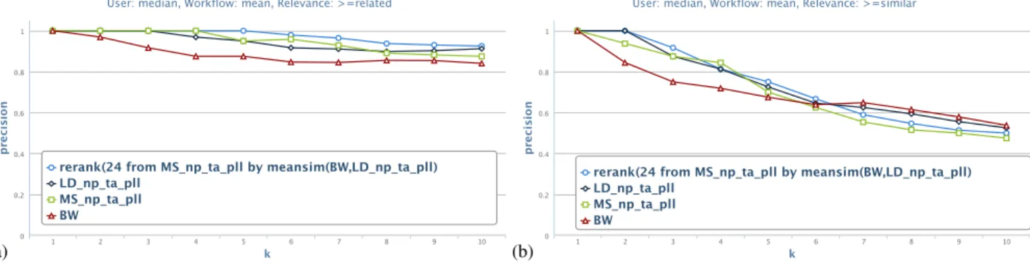
D. Reranked Retrieval Results
Given the findings regarding the deterred runtime of simLD and the fact that external knowledge to be used in
workflow comparison such as ip and te incurs a severe data acquisition bottleneck, we speculated whether the results of the (fast) Module Set comparison algorithm can be improved - without external knowledge - by merging them with the high-quality ranking performance of simLD. We therefore
performed an experiment where we reranked the top retrieval results of simM S by the ensemble of simBW and simLD.
Figure 10 shows retrieval precision for simM S, simLD, and
simBW on their own, and for the reranked top 24 search
results of simM S. Especially for the relevance threshold of
related, reranking the results clearly improves performance
and makes it comparable to that of algorithm configurations including external knowledge. For a threshold of similar, the benefit is less pronounced, yet still observable. We believe that studying in more detail such reranking methods, especially focussing on the trade-off between runtime and result quality, are a prospective venue for further research.
E. Applicability to Other Datasets
Our gold standard corpus also includes a second set of workflows from another workflow repository, namely the public Galaxy workflow repository. For 8 query workflows, rated lists of compared workflows are available to evaluate ranking performance. This dataset differs from the previous one in various respects: Galaxy workflows are exclusive to the Bioinformatics area, the repository is smaller and curated by a smaller group of people, the annotation is generally more sparse (no tags etc.), and the modules used are only local executables (no web services as frequently used in Taverna). Looking at such diverse data sets is important to show robustness of any evaluation results.
Figure 11 shows ranking correctness for simM S, simLD,
and simP S on this second dataset. The module comparison
schemes used are gw1, comparing a selection of attributes with uniform weights, and gll, comparing only module labels by their edit distance. While results are generally less good than on the myExperiment data set, simLD here even more
clearly outperforms the other algorithms. We are currently looking to extend this dataset to be able to perform a more complete evaluation and to trace back the observed differences in ranking performance to properties of the data set.
VI. CONCLUSION
We introduced Layer Decompositon (LD), a novel approach for workflow comparison specifically tailored to measuring the similarity of scientific workflows. We comparatively evaluated this algorithm against a set of state-of-the art contenders in terms of workflow ranking and retrieval. We showed that LD provides the best results in both tasks, and that it does so across a variety of different configurations - even those not requiring extensive external knowledge. Results in ranking could be confirmed using a second data set. Considering runtime, we not only showed our algorithm to be faster than other structure-aware approaches, but demonstrated how different algorithms can be combined to reduce the overall runtime while achieving comparable, or even improved result quality.
k pr ec is io n
User: median, Workflow: mean, Relevance: >=related
rerank(24 from MS_np_ta_pll by meansim(BW,LD_np_ta_pll) LD_np_ta_pll MS_np_ta_pll BW _____________ 1 2 3 4 5 6 7 8 9 10 0 0.2 0.4 0.6 0.8 1 (a) k pr ec is io n
User: median, Workflow: mean, Relevance: >=similar
rerank(24 from MS_np_ta_pll by meansim(BW,LD_np_ta_pll) LD_np_ta_pll MS_np_ta_pll BW _____________ 1 2 3 4 5 6 7 8 9 10 0 0.2 0.4 0.6 0.8 1 (b)
Fig. 10: Mean retrieval precision at k against the median expert rating for similarity algorithms MS, LD and BW, and the top 24 results of MS reranked by the ensemble of BW and LD, for relevance threshold (a) related, and (b) similar.
al go ri th m s ranking correctness
User: BioConsert5, Workflow: mean
-0.4 -0.2 0 0.2 0.4 0.6 0.8 1 PS_gll: 0.39 PS_gw1: 0.385 LD_gll: 0.465 LD_gw1: 0.465 MS_gll: 0.357 MS_gw1: 0.42
Fig. 11: Mean ranking results on Galaxy workflows (see text).
Though we did consider runtimes, our evaluation clearly focusses on the quality of ranking and retrieval. Real-time similarity search at repository-scale will require further efforts in terms of properly indexing workflows. Such indexing of workflows is straightforward when considering only their modules (like in simM S), but requires more sophisticated
methods when also topology should be indexed. Therefore, our approach of stacking Layer Decomposition-based ranking onto workflow retrieval by modules provides a good starting place for applying structure-based workflow similarity to scientific workflow discovery to scale.
ACKNOWLEDGMENT
This work was partly funded by DFG grant GRK1651, DAAD grants D1240894 and 55988515, and PHC Procope grant. Work of SCB partly done in the context of the Institut de Biologie Computationnelle, Montpellier, France.
REFERENCES
[1] P. Mates, E. Santos, J. Freire, and C. Silva, “Crowdlabs: Social analysis and visualization for the sciences,” SSDBM, pp. 555–564, 2011. [2] “SHIWA workflow repository,” http://shiwa-repo.cpc.wmin.ac.uk. [3] J. Goecks, A. Nekrutenko, and J. Taylor, “Galaxy: a comprehensive
approach for supporting accessible, reproducible, and transparent com-putational research in the life sciences.” Genome Biology, vol. 11, no. 8, p. R86, 2010.
[4] D. Roure, C. Goble, and R. Stevens, “The design and realisation of the myexperiment virtual research environment for social sharing of workflows,” Future Generation Computer Systems, vol. 25, no. 5, pp. 561–567, 2009.
[5] S. Cohen-Boulakia and U. Leser, “Search, Adapt, and Reuse: The Future of Scientific Workflow Management Systems,” SIGMOD Record, vol. 40, no. 2, pp. 6–16, 2011.
[6] A. Goderis, P. Li, and C. Goble, “Workflow discovery: the problem, a case study from e-Science and a graph-based solution,” ICWS, pp. 312–319, 2006.
[7] R. Bergmann and Y. Gil, “Similarity assessment and efficient retrieval of semantic workflows,” Information Systems, vol. 40, pp. 115–127, 2012.
[8] N. Friesen and S. R¨uping, “Workflow Analysis Using Graph Kernels,” SoKD, 2010.
[9] E. Santos, L. Lins, J. Ahrens, J. Freire, and C. Silva, “A First Study on Clustering Collections of Workflow Graphs,” IPAW, pp. 160–173, 2008. [10] V. Silva, F. Chirigati, K. Maia, E. Ogasawara, D. Oliveira, V. Bragan-holo, L. Murta, and M. Mattoso, “Similarity-based Workflow Cluster-ing,” CCIS, vol. 2, no. 1, pp. 23–35, 2010.
[11] J. Stoyanovich, B. Taskar, and S. Davidson, “Exploring repositories of scientific workflows,” WANDS, pp. 7:1–7:10, 2010.
[12] X. Xiang and G. Madey, “Improving the Reuse of Scientific Workflows and Their By-products,” ICWS, pp. 792–799, 2007.
[13] F. Costa, D. d. Oliveira, E. Ogasawara, A. Lima, and M. Mattoso, “Athena: Text Mining Based Discovery of Scientific Workflows in Disperse Repositories,” RED, pp. 104–121, 2010.
[14] J. Starlinger, B. Brancotte, S. Cohen-Boulakia, and U. Leser, “Similarity Search for Scientific Workflows,” PVLDB, vol. 7, no. 12, 2014. [15] J. Corrales, D. Grigori, and M. Bouzeghoub, “BPEL Processes
Match-making for Service Discovery,” CoopIS, 2006.
[16] J. Krinke, “Identifying similar code with program dependence graphs,” WCRE, pp. 301–309, 2001.
[17] F. Malucelli, T. Ottmann, and D. Pretolani, “Efficient labelling al-gorithms for the maximum noncrossing matching problem,” Discrete Applied Mathematics, vol. 47, no. 2, pp. 175–179, 1993.
[18] J. Starlinger, S. Cohen-Boulakia, and U. Leser, “(Re)Use in Public Scientific Workflow Repositories,” SSDBM, pp. 361–378, 2012. [19] R. Likert, “A technique for the measurement of attitudes,” Archives of
Psychology, 1932.
[20] S. Cohen-Boulakia, A. Denise, and S. Hamel, “Using medians to generate consensus rankings for biological data,” SSDBM, pp. 73–90, 2011.
[21] W. Cheng, M. Rademaker, B. Baets, and E. H¨ullermeier, “Predicting partial orders: ranking with abstention,” ECML/PKDD, pp. 215–230, 2010.
[22] F. McSherry and M. Najork, “Computing information retrieval perfor-mance measures efficiently in the presence of tied scores,” Advances in Information Retrieval, 2008.
[23] I. Wassink, P. Vet, K. Wolstencroft, P. Neerincx, M. Roos, H. Rauwerda, and B. T.M., “Analysing Scientific Workflows: Why Workflows Not Only Connect Web Services,” Services, pp. 314–321, 2009.
![Fig. 2: Workflow comparison process, see also [14]](https://thumb-eu.123doks.com/thumbv2/123doknet/13968019.453483/3.918.76.451.83.333/fig-workflow-comparison-process-see-also.webp)