HAL Id: hal-01058278
https://hal.inria.fr/hal-01058278
Submitted on 26 Aug 2014HAL is a multi-disciplinary open access
archive for the deposit and dissemination of sci-entific research documents, whether they are pub-lished or not. The documents may come from teaching and research institutions in France or abroad, or from public or private research centers.
L’archive ouverte pluridisciplinaire HAL, est destinée au dépôt et à la diffusion de documents scientifiques de niveau recherche, publiés ou non, émanant des établissements d’enseignement et de recherche français ou étrangers, des laboratoires publics ou privés.
Quantifying and localizing state uncertainty in hidden
Markov models using conditional entropy profiles
Jean-Baptiste Durand, Yann Guédon
To cite this version:
Jean-Baptiste Durand, Yann Guédon. Quantifying and localizing state uncertainty in hidden Markov models using conditional entropy profiles. COMPSTAT 2014 - 21st International Conference on Computational Statistics, The International Association for Statistical Computing (IASC), Aug 2014, Genève, Switzerland. pp.213-221. �hal-01058278�
uncertainty in hidden Markov
models using conditional entropy
profiles
Jean-Baptiste Durand, Univ. Grenoble Alpes, LJK and Inria, Mistis, F-38000 Grenoble, France, [email protected]
Yann Gu´edon, CIRAD, UMR AGAP and Inria, Virtual Plants, F-34095 Montpellier, France, [email protected]
Abstract. A family of graphical hidden Markov models that generalizes hidden Markov chain (HMC) and tree (HMT) models is introduced. It is shown that global uncertainty on the state process can be decomposed as a sum of conditional entropies that are interpreted as local contributions to global uncertainty. An efficient algorithm is derived to compute conditional entropy profiles in the case of HMC and HMT models. The relevance of these profiles and their complementarity with other state restoration algorithms for interpretation and diagnosis of hidden states is highlighted. It is also shown that classical smoothing profiles (posterior marginal probabilities of the states at each time, given the observations) cannot be related to global state uncertainty in the general case.
Keywords. Hidden Markov models, State inference, Conditional entropy.
1
Introduction
Hidden Markov models (HMMs) have been used frequently in sequence analysis for modeling various types of latent structures, such as homogeneous zones or noisy patterns (Ephraim & Mehrav, 2002). They have been extended from sequences to more general structures, particularly tree structures. In HMMs, inference for model parameters can be distinguished from inference for the state process given parameters. This work focuses on state process inference.
State inference is particularly relevant in numerous applications where the unobserved states have a meaningful interpretation. In such cases, the state sequence has to be restored. The restored states may be used, typically, in prediction, in segmentation or in denoising (Ephraim
2 Conditional entropy profiles for hidden Markov models & Mehrav, 2002). Such use of the state sequence relies on the assumption that uncertainty on the state process given observations should be reasonably low. Not only is state restoration essential for model interpretation, it is generally used for model diagnostic and validation as well, for example by visualising some functions of the states – typically, to compare histograms with conditional densities given the states. The use of restored states in the above-mentioned contexts makes assessment of state sequence uncertainty a critical step of the analysis.
Global quantification of such uncertainty has been addressed by Hernando et al. (2005). However, this is insufficient for detailed state interpretation: knowledge of the distribution of that global uncertainty along the structure is also of primary importance. Quantification of local state uncertainty given observed sequence X = x for a known HMC model has been adressed by either enumeration of state sequences, or by state profiles, which are state sequences summarised in a K × T array, T being the sequence length and K the number of states (Gu´edon, 2007).
We here address quantification of state uncertainty in an HMM with observed process X = (Xv)v∈V indexed by a fixed Directed Acyclic Graph (DAG) G with vertex set V and edge set E. This family of HMMs is referred to as graphical hidden Markov models (GHMMs). This family contains hidden Markov chain (HMC) and tree (HMT) models. Let S = (Sv)v∈V denote the associated hidden state process, Sv taking values in the set {0, . . . , K − 1}. Let x be a possible realization of X. Let pa(v) denote the parent of vertex v and for any subset U of V, let XU (resp. xU) denote the family of random variables (Xu)u∈U (resp. observations (xu)u∈U). It is assumed that: S satisfies the Markovian factorization property associated with DAG G, where the vertex set V is assimilated to the family of random variables (Sv)v∈V (Lauritzen, 1996); the distribution of S is parametrized by the transition probabilities pspa(v),k = P (Sv = k|Spa(v) = spa(v)) and for the source vertices (vertices with no parent) u in G, by the initial probabilities (P (Su = k))k; given S, the random variables (Xv)v are independent and Xu is independent from (Sv)v6=u.
Usually, profiles of smoothed probabilities (P (Sv = k|X = x))v∈V with k = 0, . . . , K − 1 have been used for quantifying state uncertainty. This approach suffers from two main short-comings: as will be shown later, perception of state uncertainty associated with those profiles leads to overestimating global uncertainty of S given X = x. Moreover, visualization of those multidimensional profiles is made difficult by the graphical nature of arbitrary DAGs G, provided that K > 2. In our approach, entropy H is considered as the canonical measure of uncertainty. Thus, H(S|X = x) quantifies state process uncertainty given observations. This entropy can be decomposed into a sum of entropies. Every term of that sum is associated with one vertex in V. Hence, these entropies can be interpreted as local contributions to global uncertainty. Since these profiles are unidimensional, they can be drawn whatever the graphical structure G. In what follows, this decomposition is made explicit. Then efficient algorithms are given in the HMC and HMT model cases to compute the elements of the decomposition. It is shown using synthetic and real-case data that the obtained local entropy profiles are relevant for state uncer-tainty diagnosis and state interpretation. These algorithms are complementary with approaches that enumerate the L most likely state restorations (so-called generalized Viterbi algorithm), and with approaches that compute profiles of alternative states to the most likely state pro-cess value. This so-called Viterbi forward–backward algorithm formally solves the optimization problem
(arg) max (su)u6=v
P ((Sv = sv)u6=v, Sv = k|X = x).
It is also shown that usual smoothed probability profiles are not relevant for quantifying global state uncertainty, due to their inherent marginalization property.
2
Conditional entropy profiles
Let X be a GHMM as defined in Section 1. It is assumed that the associated hidden state process S satisfies the factorization associated with the Markov property on G :
∀s, P (S = s) = Y v∈V
P (Sv = sv|Spa(v)= spa(v)), (1)
where P (Sv = sv|Spa(v)= spa(v)) refers to P (Ss = ss) if pa(v) = ∅.
The decomposition of entropy H(S|X = x) comes from the conditional distribution of S given X = x also satisfying the factorization property of G:
P (S = s|X = x) =Y v
P (Sv = sv|Spa(v) = spa(v), X = x),
with the same convention as before if pa(v) = ∅.
Proof. This property is proved by induction on the vertices of G (as would be proved factorization (1)). The random variables (S, X) satisfy the Markov property on DAG G′ which edge set E′ is defined as a ∈ E′ ⇔ {[a = (Su, S
v) and (u ∈ pa(v))] or a = (Su, Xu)}. Let u in G be a sink vertex (vertex without children): then Su is separated from (Sv)v6=u,v /∈pa(u) by Spa(u) in the moral graph of G′. Thus, the following factorization holds:
P (S = s|X = x) = P (Su = su|Spa(u) = spa(u), X = x)P ((Sv)v6=u= (sv)v6=u|X = x).
The additive decomposition of entropy is obtained by applying the chain rule (Cover & Thomas, 2006, chap. 2)
H(S|X = x) =X v
H(Sv|Spa(v), X = x), (2)
with the same convention as before if pa(v) = ∅. As a consequence, the global state process uncertainty is decomposed as a sum of conditional entropies (H(Sv|Spa(v), X = x))v∈V, which define an entropy profile. Hence, each term of the sum is interpreted as a local uncertainty that contributes additively to global uncertainty.
In contrast, marginal entropies (H(Sv|X = x))v∈V quantify uncertainty associated with smoothed probabilities ξv(k) = P (Sv = k|X = x) for v ∈ V and 0 ≤ k < K. These marginal entropies are upper bounds of the conditional entropies (Cover & Thomas (2006), chap. 2). Hence,
H(S|X = x) ≤X v
H(Sv|X = x).
As a consequence, smoothed probability profiles do not represent uncertainty on the value of S. The particular case of HMC models is considered. Here G is a linear graph with T vertices, and for any t < T , X0 = x0, . . . , Xt= xtis denoted by X0t = xt0. Here (2) can be rewritten as
H(S|X = x) = H(S0|X = x) + T −1X
t=1
4 Conditional entropy profiles for hidden Markov models with
H(St|St−1, X = x) = −X i,j
P (St= j, St−1 = i|X = x) log P (St= j|St−1= i, X = x).
This results from definition H(St|St−1, X = x) = E[− log P (St|St−1, X = x)], where expec-tation is under P (St, St−1|X = x). The usual forward recursion computes αt(j) = P (St = j|Xt
0 = xt0) and γt(j) = P (St = j|X0t−1 = xt−10 ) for each time t and each state j and com-bine them in the backward recursion to yield the smoothed probabilities ξt(j) = P (St = j| X = x). Thus, computation of the conditional entropy profile H(St|St−1, X = x) with 0 < t ≤ T − 1 can be integrated in the backward recursion by computing P (St = j| St−1 = i, X = x) = ξt(j)pijαt−1(i)/{γt(j)ξt−1(i)} where pij = P (St = j|St−1 = i) is the transition probability. This approach can be seen as an alternative to the algorithm of Her-nando et al. (2005). It allows the computation of H(S|X = x) with the same complexity in O(T K2), but the advantage of our approach is to provide the conditional entropy profile.
In the case of HMTs indexed by tree G = T the smoothed probabilities ξv(k) = P (Sv = k| X = x) are computed for v ∈ T by an upward–downward algorithm. A numerically stable iterative algorithm was proposed by Durand et al. (2004). It relies on an upward recursion, initialized at the leaf vertices of T . The computed quantities are βv(k) = P (Sv = k| ¯Xv = ¯xv) and βpa(v),v(k) = P ( ¯Xv = ¯xv|Spa(v) = k)/P ( ¯Xv = ¯xv) for each vertex v and each state j, where ¯Xv denotes the subtree rooted in v. These quantities are computed as a function of βu and βpa(u),u for the children u of v. The algorithm complexity is in O(K2) per iteration. The smoothed probabilities are computed using a downward recursion initialized at the root vertex of T . In this recursion, the ξv(k) are computed as a function of ξpa(v), βv and βpa(v),v. The complexity is in O(K2) per iteration as well. Similarly to the HMC case, adding the computation of
H(Sv|Spa(v), X = x) = − X
i,j
P (Sv = j, Spa(v)= i|X = x) log P (Sv = j|Spa(v)= i, X = x)
to the downward recursion, with P (Sv = j|Spa(v)= i, X = x) = βv(j)pij/{P (Sv = j)βpa(v),v(i)} and pij = P (Sv = j|Spa(v)= i), allows for extracting conditional entropy profiles, while keeping the complexity per iteration of the algorithm in O(K2).
3
Applications
Synthetic examples
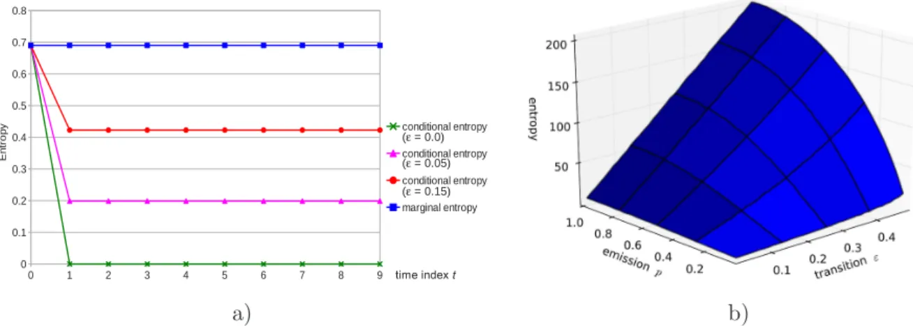
A two-state HMC family is considered. Its transition probability matrix is parametrized by ε = P (St = 1|St−1 = 0) = P (St = 0|St−1 = 1), ε ∈ [0, 0.5]. The initial state distribution π is P (S0 = 0) = P (S0 = 1) = 0.5. The observation process takes values in {0, 1, 2} and the emission distributions (conditional probabilities of observations given the states) are P (Xt = 0|St = 0) = 1 − p; P (Xt = 1|St = 0) = p; P (Xt = 1|St = 1) = p; P (Xt = 2|St= 1) = 1 − p where p ∈ [0, 1] is an additional parameter.
In a first experiment, p is fixed at 0.5 and the considered observed sequence is xt = 1 for t = 0, . . . , T − 1. The smoothed probabilities are ξt(0) = ξt(1) = 0.5 for t = 0, . . . , T − 1. Thus, for any value of ε, marginal entropy is log 2 and the sum of these entropies over t is T log 2. In
contrast, global entropy of the hidden state sequence is a strictly increasing function of ε. Its minimum log 2 is reached for ε = 0, whereas its maximum T log 2 is reached for ε = 0.5.
Marginal and conditional entropy profiles are represented in Figure 1 a). For ε = 0, the conditional entropy profile is interpreted as follows: global uncertainty is log 2, which corre-sponds to uncertainty concerning the first state only. Given this first state, every subsequent state is deterministic and does not contribute to global uncertainty. The marginal entropy pro-file highlights equiprobability of both states at each time t given the observations. The same statement would hold under an independent mixture assumption for (Xt)t≥0. Marginal entropy results from uncertainty concerning state St due to observing Xt= xt, but also to propagation of uncertainty from past states. As a consequence, marginal entropy cannot be interpreted in terms of local contributions to global uncertainty. In contrast, conditioning by the past state in entropy withdraws the effect of uncertainty propagation.
In a second experiment, the effect of p and ε on global state entropy is assessed by simulating 100 sequences of length T = 300 for each p ∈ [0, 1] and each ε ∈ [0, 0.5] on a regular grid with 40 × 40 points. The mean global entropy over the 100 sequences is represented in Figure 1 b). As expected, entropy increases with the emission distribution overlapping (p → 1) and as the rows of the transition probability matrix tend to π (ε → 0.5), so that maximal entropy T log 2 is obtained in the independence case ε = 0.5 with full overlapping p = 1.0.
a) b)
Figure 1. a) Marginal and conditional entropy profiles for a 2-state HMC model with transition probabilities ε = 0.0, ε = 0.05 and ε = 0.15. b) Mean global state entropy for simulated sequences as a function of transition probability ε and emission probability p.
Analysis of the structure of Aleppo pines
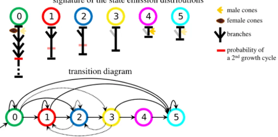
The aim of this study was to build a model of the architectural development of Aleppo pines. The dataset contained seven branches of Aleppo pines, issued from different individuals. They were described at the scale of annual shoots v (segment of stem established within a year). Each branch was assimilated with a (mathematical) tree. Each tree vertex v (shoot) was characterized through one observed 5-dimensional vector Xv composed of the: number of growth cycles (from 1 to 3), presence of male sexual organs (binary variable), presence of female sexual organs (binary variable), length in cm, number of branches per tier. The parameters were estimated by maximum likelihood using the EM algorithm. The number of states was chosen by the ICL-BIC criterion (see Section 4), leading to selection of a 6-state HMT model. The Markov
6 Conditional entropy profiles for hidden Markov models tree is initialized in state 0 with probability one. A summary of the state transitions and an interpretation of the hidden states are provided in Figure 2.
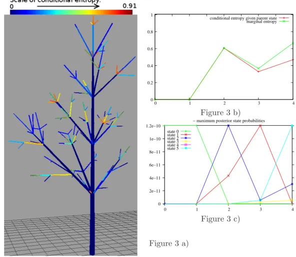
As a first step, profiles of conditional entropies were represented using a colormap (mapping between entropy values and color intensities) – see Figure 3 a). This step highlighted location of the vertices with least ambiguous states along the branch main axes, and location of the vertices with most ambiguous states at the peripheral parts of branches. Then, state profiles were drawn along paths extending from the root vertex to leaf vertices. These paths were chosen so as to contain vertices with high conditional entropies. On the one hand, a detailed analysis of state uncertainty along the paths were obtained by Viterbi upward–downward profiles. This provided local alternative state values to the most likely tree states given by the Viterbi algorithm. On the other hand, the generalized Viterbi algorithm was used to characterize how clusters of neighbor vertices had simultaneous state changes in alternative state configurations. These results highlighted that the paths with most ambiguous states were composed of successions of unbranched, sterile shoots with one single growth cycle.
Figure 2. 6-state HMT model: transition diagram and symbolic representation of the state sig-natures (conditional mean values of the variables given the states, depicted by typical shoots). The separation between growth cycle is represented by a horizontal red segment, which intensity is proportional to the probability of occurrence of a second growth cycle. Dotted arrows cor-respond to transitions with associated probability < 0.1. Mean shoot lengths given each state are proportional to segment lengths, except for state 0 (which mean length is slightly more than twice the mean length for state 1).
The application of this methodology is illustrated below on a path containing successive monocyclic, sterile shoots. This path belongs to the fourth individual (for which H(S|X = x) = 47.5). It is composed by 5 vertices, referred to as {0, . . . , 4}. Shoots 0 and 1 are long and highly branched, and thus are in state 0 with probability ≈ 1 (also, shoot 0 is bicyclic). Shoots 2 to 4 are monocyclic and sterile. Shoots 2 and 3 bear one branch, and can be in states 1 or 2 essentially. Shoot 4 is unbranched and from the Viterbi profiles in Figure 3c), it can be in states 2, 3 or 5. This is summarized by the conditional entropy profile in Figure 3b).
This conditional entropy profile can be further interpreted, in relation with mutual infor-mation I(Su; Spa(u)|X = x). On the one hand, I(S1; S2|X = x) = 0. This results from state S1 being known. Thus, conditioning by S1 does not provide further information on its children state S2. On the other hand, I(S3; S4|X = x) = 0.2. Uncertainty associated with the posterior
distribution of S4 is high, since H(S4|X = x) = 0.67. However, knowledge of its parent state S3 would reduce the uncertainty on S4: if S3 = 1 then S4 = 5; if S3 = 2 then S4 = 2 (or less likely, S4= 3) and if S3 = 3 then S4 = 5 (or less likely, S4= 2).
Using an extension of (2) to subgraphs of T , the contribution of the vertices of the considered path P to global state tree entropy can be computed asPu∈PH(Su|Spa(u), X = x) and is equal to 1.41 in the above example (that is, 0.28 per vertex on average). The global state tree entropy for this individual is 0.24 per vertex, against 0.20 per vertex in the whole dataset. This is explained by the lack of information brought by the observed variables (several successive sterile monocyclic shoots, which can be in states 1, 2, 3 or 5).
The contribution of P to the global state tree entropy corresponds to the sum of the heights of every point of the profile of conditional entropies in Figure 3b).
Note that the representation of state uncertainty using profiles of posterior state probabilities induces a perception of global uncertainty on the states along P equivalent to that provided by marginal entropy profile in Figure 3b). The mean marginal state entropy for this individual is 0.37 per vertex, which strongly overestimates the global state tree entropy per vertex (0.24).
0 0.2 0.4 0.6 0.8 1 0 1 2 3 4
conditional entropy given parent state marginal entropy Figure 3 b) 0 2e−11 4e−11 6e−11 8e−11 1e−10 1.2e−10 0 1 2 3 4
− maximum posterior state probabilities
state 0 state 1 state 2 state 3 state 4 state 5 Figure 3 c) Figure 3 a)
Figure 3. a) Conditional entropy profiles H(Su|Spa(u), X = x) for vertices u associated with one of the seven branches. Blue corresponds to lowest and red to highest conditional entropies. b) Profiles of conditional and of marginal entropies along a path containing mainly sterile mono-cyclic shoots. c) State tree restoration with the Viterbi upward-downward algorithm.
8 Conditional entropy profiles for hidden Markov models
4
Concluding remarks
In this work, conditional entropy profiles are proposed to assess both local and global state uncertainty in GHMMs. As shown in the examples, these profiles allow deeper understanding of the local roles of the model parameters, the neighbouring states and the observed data, concerning state uncertainty. These profiles are a valuable tool to analyse alternative state restorations, which may involve zones of connected vertices. Such situations are characterised by high mutual information between connected vertices. Moreover, the examples highlight that the posterior state probability profiles introduce confusion between (i) local state uncertainty due to overlap of emission distributions for different states and (ii) mere propagation of uncertainty from past to future states. Contrary to conditional entropy profiles, they suggest strong local contributions to global state uncertainty in zones where such uncertainty is in fact far more limited.
In the perspective of model selection, entropy may also be useful. If irrelevant states or variables are added to GHMMs, global state entropy is expected to increase. This explains why several model selection criteria based on a compromise between log-likelihood and state entropy were proposed. Among these is the Normalised Entropy Criterion introduced by Celeux & Soromenho (1996) in independent mixture models, and ICL-BIC introduced by McLachlan & Peel (2000, chap. 6). Their generalization to GHMMs is rather straightforward. By favouring models with small state entropy and high log-likelihood, these criteria aim at selecting models such as the uncertainty of the state values is low, whilst achieving good fit to the data.
Bibliography
[1] Celeux, G., and Soromenho, G. (1996) An entropy criterion for assessing the number of clusters in a mixture model. Classification Journal, 13, 195–212.
[2] Cover, T., and Thomas, J. (2006) Elements of Information Theory, 2nd edition. Hoboken, NJ: Wiley.
[3] Durand, J.-B., Gon¸calv`es, P., and Gu´edon, Y. (Sept. 2004) Computational Methods for Hidden Markov Tree Models – An Application to Wavelet Trees. IEEE Transactions on Signal Processing, 52, 9, 2551–2560.
[4] Ephraim, Y., and Merhav, N. (June 2002) Hidden Markov processes. IEEE Transactions on Information Theory, 48, 1518–1569.
[5] Gu´edon, Y. (2007) Exploring the state sequence space for hidden Markov and semi-Markov chains. Computational Statistics and Data Analysis, 51, 5, 2379–2409.
[6] Hernando, D., Crespi, V., and Cybenko, G. (2005) Efficient computation of the hidden Markov model entropy for a given observation sequence. IEEE Transactions on Information Theory, 51, 7, 2681–2685.
[7] Lauritzen, S. (1996) Graphical Models. Clarendon Press, Oxford, United Kingdom.
[8] McLachlan, G., and Peel, D. (2000) Finite Mixture Models. Wiley Series in Probability and Statistics. John Wiley and Sons.