APPLICATION OF SATELLITE CLOUD-MOTION VECTORS IN HURRICANE TRACK PREDICTION
by
Alan L. Adams
B.A.E., Georgia Institute of Technology (1971)
B.E.S., University of Texas (1972)
Submitted in partial fulfillment of the requirements for the degree of
Master of Science at the
Massachusetts Institute of Technology
f , ...
, "
/1
1
I
/
Signature
Certified by.
of Author . *oo • * **-o'o •... .... 0***
Department of Meteorology, Jan. 21, 1976 Thesis Supervisor
Thesis Supervisor
Accepted by... ... ... ....o....*...o
Chairman, Departmental Committee
SL ren
-2-APPLICATION OF SATELLITE CLOUD-MOTION VECTORS IN HURRICANE TRACK PREDICTION
by
Alan L. Adams
Submitted to the Department of Meteorology on January 1976 in partial fulfillment of the
requirements for the degree of Master of Science.
ABSTRACT
The representation of the mean tropospheric flow by satellite -derived cloud-motion vectors is studied for use in a barotropic hurricane prediction model. The systematic use of these vectors is considered over areas not covered by rawinsonde data to aid the initial analysis of the flow pattern. Linear regression analysis is used to develop equations for the pressure-averaged tropospheric flow from data at only 1, 2, or 3 levels. The equations are derived from a large sample of
rawinsonde observations, used as simulated cloud-motion vectors, from the tropical and subtropical latitudes of the Northern Hemisphere. The performance of the regression equations on independent data is considered, as is the loss of skill when satellite winds are used
in the equations instead of rawinsonde winds. The satellite data is applied, ina pilot study, to two
operational SANBAR hurricane forecasts, with inconclusive results.
Thesis Supervisor: Frederick Sanders
Professor of Meteorology
~I~1L1 I-L~?.~YI~--F1Q IPI1-XI~ 1II~_-~1-~_
-3-TABLE OF CONTENTS
List of Tables....,,...
List of Figures... ..e.e.e...ee... I. Introduction... .g... II. Satellite-Derived Winds...
III. Data Samples For Regression Analysis... IV. Linear Regression Analysis....,... V. Results of Linear Regression Analysis...
Page 4 5 6 8 10 14 15 VI. Comparability of Satellite Data to Rawinsonde
Data...,...
VII. Selection of Operational VIII. Results of Test Cases... Acknowledgements... References...,,...,,, Appendix A... Appendix B... Appendix C... Appendix D... Appendix E... Appendix F... Appendix G... Appendix H...o...o... Cases For .. 00000000 e... 00000... 000 g... ... g.e.0. .ee... .... 0..0. . 0 .000 0 0 0 0 0 0 0 0 00 0 * * 0 *0 0 0 0 * 0 0 0 0 0 00 0 0 0 0 0 * 0 0 0* 000 0 0 * 0 0 0 0..00..0000.000 ... Study. g.e... . *e. g.e... .0.... 0... ... ... ... 24 29 32 36 38 39 41 42 44 48 49 53 57 c... e00 0 .... 00.00 0.000 0000 .... .... 0
-4-LIST OF FIGURES
Page
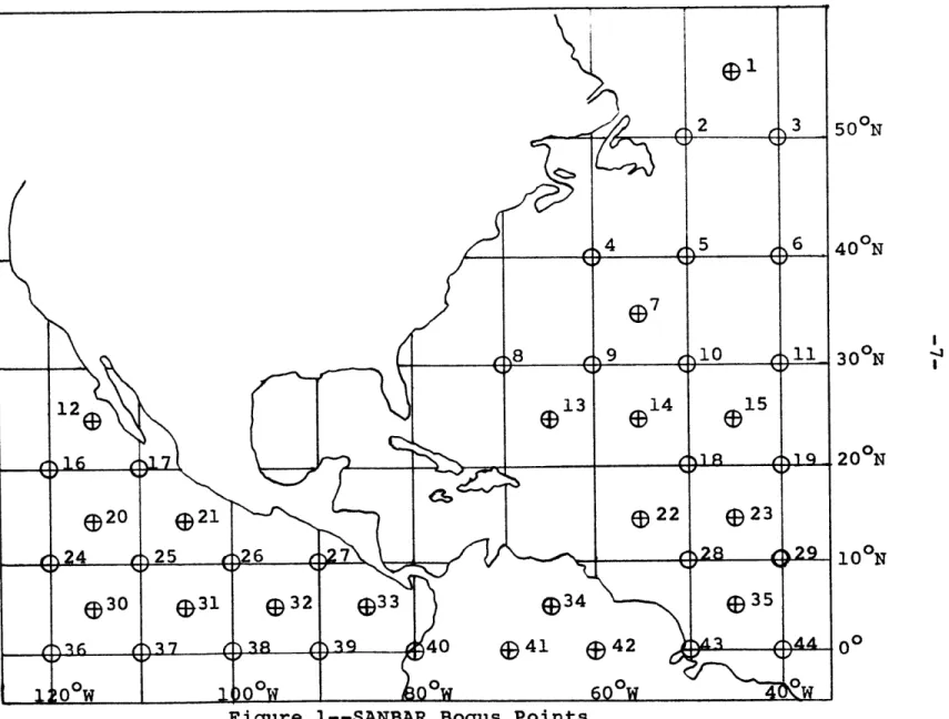
i, SANBAR Bogus Points, ... o 7
2. Locations of Regression Analysis Data Stations
Relative To 850-mb Average Flow... 12 3. Locations of Regression Analysis Data Stations
Relative To 200-mb Average Flow... 13
4. Elaine Forecasts From September 10, 1974,
1200GMT.oEl....a.in..e.oF...orcat...sb...e** 34
5. Elaine Forecasts From September 11, 1974,
1200GIT ..o ...o.o.o... 35
-
-5-LIST OF TABLES
Page
1. Stations For Linear Regression Analysis....,.... 11 2. Data Stratificationso... 18 3. Regression Equation Results, Geographical
Stratifications, u Component... 20 4. Regression Equation Results, Geographical
Stratifications, v Component...,.,,... 21 5. Regression Equation Results, Time
Stratification...oe... 22 6. Standard Deviations of The Mean Wind...5. 23 7. Effects of Satellite Data Error...,... 27 8. Forecast Results For Tropical Storm Elaine... 33
-6-I. INTRODUCTION
SANBAR is a barotropic hurricane prediction model that utilizes vorticity conservation in the mean trop-ospheric flow to predict tracks of tropical cyclones. The model was developed by Sanders and Burpee (1968) and has been discussed by Sanders (1970) and by Sanders et al (1975). SANBAR makes use of observed winds which are averaged with respect to pressure through the depth of the troposphere, defined as the layer between the 1000-mb and 100-mb surfaces. The averaged wind is represented by the weighted average of the data at the ten mandatory levels, as observed by rawinsonde.
A major factor limiting forecast accuracy in the operational use of the model at the Natiohal Hurricane Center (NHC) was the lack of data over the large oceanic areas included in the SANBAR forecast grid area.
Sanders et al (1975) discussed specific cases. To guide the analysis of the wind field over the vast oceanic areas far from any rawinsonde observations, the model relies on "bogus" wind observations at 44 selected geographical locations. These bogus points are shown in Figure 1. The winds are obtained at present from consideration of many factors, including
12-hour prognostic wind and height fields, surface observations from ships, aircraft reports, and SMS satellite-derived winds. This report explores the increased and systematic use of such satellite winds over the oceans to improve the initial analysis, by determining how well the pressure-averaged flow is represented by information at one, two, or three
500N
40oN
30oN
200 N
10 N
-8-II. SATELLITE-DERIVED WINDS
The use of satellite photographs to track cloud motion as a means of determining wind velocity at
cloud level was discussed by Hubert and Whitney (1971). They compared cloud movements from the geostationary ATS satellite imagery with rawinsonde observations of wind from nearby stations. Reasonable agreement was found, if the motions of low level and high level clouds were compared to winds in the layers from
3000 to 5000 feet and around 30,000 feet, respectively. EOn rare occasions when mid-level clouds can be
identified, their wind vectors are assigned to the 500 mb level by the National Meteorological Center. (NMC).] The median vector differences between these estimated and rawinsonde observations at low and high levels are approximately 6 knots and 12 knots,
respec-tively (Hubert, 1975). Further discussion of satellite derived winds can be found in Appendix A.
Given good satellite coverage, it is thus possible to obtain estimates of wind flow at low levels and high levels over wide areas with possibly some idea of the mid-level flow. This information should be extremely valuable over oceanic regions for prediction of tracks of tropical storms. In the context of the SANBAR model, the question then arises how adequately one, two, or three levels of wind data can represent the mean
tropospheric flow. Linear regression analysis will be used to estimate the mean flow from rawinsonde obser-vations (used as simulated cloud-motion vectors) at one to three levels.
The idea of using satellite cloud-motion vectors to improve the bogus data is not new. Pike (1975),
-9-at NHC, developed a set of regression equ-9-ations utilizing data from the low level ATOLL (Atlantic Tropical Oceanic Lower Layer) analysis and the 200 mb analysis. The ATOLL analysis is essentially the level at the top of the planetary boundary layer and utilizes ship reports, low-level satellite winds, and available 2000-foot rawinsonde winds. The 200-mb analysis is supplemented with aircraft observations and upper
level satellite winds. Pike's equations for June through November are included in the section on results from
linear regression analysis. They are applied to a small sample of data in the Western Atlantic,
Carribean Sea, and Gulf of Mexico.
The purpose of this report is to first develop a statistically stable set of linear regression
equations from a substantially larger sample of data over time and geographical location than used by Pike. The results of the linear regression analysis will then
be applied to the initial data field in operational SANBAR cases, in hopes of improving the forecasts. Only satellite winds will be used at low levels while
the high-level data will consist of satellite winds and aircraft reports.
~--~I~L--
-10-III. DATA SAMPLE FOR REGRESSION ANALYSIS
The data for the linear regression analysis consist of a sample of rawinsonde observations from 20 stations located between 00 and 35oN and 60oW westward to 1300E, as listed in Table 1. The data sample is for the months of June through October from 1971 through 1974 for each of the 20 stations. The five-month period corresponds to the period of maximum tropical storm activity in the data area. The five-year time span was chosen to create a sample of sufficient size to obtain statistically sound
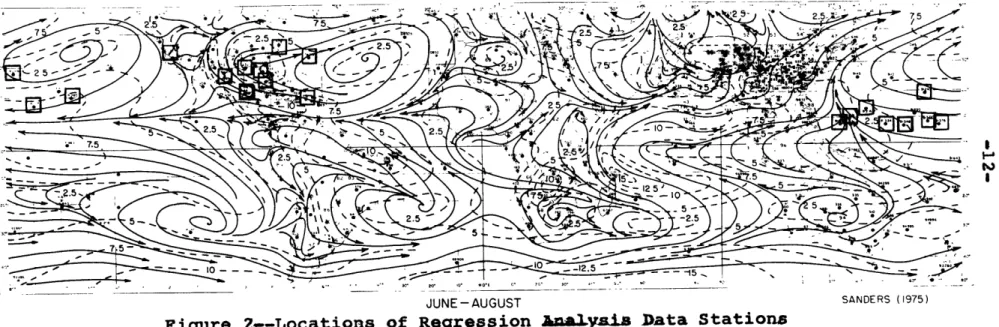
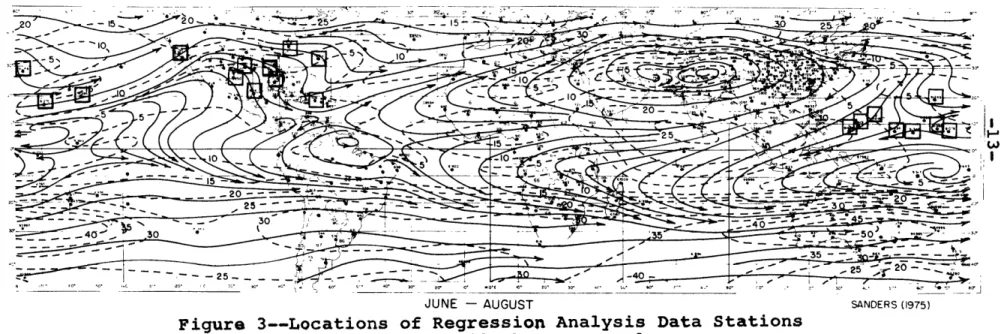
results, even after considerable stratification. The 20 stations were chosen to provide coverage of different wind regimes and areas of tropical storm activity. The stations are shown in Figures 2 and 3 relative to the long-term mean June-August streamline pattern for the 850-mb and 200-mb levels respectively. The streamline analyses are based on data from
-11-TABLE 1
Stations For Linear Regression Analysis
Int.
Index No. Station Name Lat. Long,
1. 78016 Bermuda 32.2N 64.6W
2. 78526 San Juan, P.R. 18.3N 66.1W 3. 72304 Cape Hatteras, N.C. 35.3N 75.6W
4. 72202 Miami, Fla. 25.5N 80.1W
5. 72211 Tampa, Fla. 27.6N 82.3W
6. 72240 Lake Charles, La. 30.2N 93.1W 7. 72250 Brownsville, Tx. 25.6N 97.3W 8. 72295 Vandenberg, Cal. 33.9N 118.4W 9. 76644 Merida, Mex. 20.6N 89.4W 10. 91285 Hilo, Hi. 19.4N 155.3W 11. 91275 Johnston Is. 17.0N 168.3W 12. 91066 Midway 28.1N 177.2W
13. 91217 Taguac, Guam 13.3N 144.5E
14. 91245 Wake Is. 19.1N 166.3E
15. 91334 Truk 7.4N 151.8E
16. 91348 Ponape 7.0ON 158.2E
17. 91366 Kwajalein 8.7N 167.6E
18. 91376 Majuro 7.1N 177.4E
19. 91413 Yap 9.3N 138.1E
LONG-TERM MEAN 850-mb FLOW. DATA FROM NEWELL(1972), LUFTHANSA(1967), SADLER(1970),nd SCHWARTZKOPF(1970). -ISOTACHS IN M SEC
-'
JUNE - AUGUST
Figure 2--Locations of Regression Analysia Data Stations R6Ielative To 850-mb Average Flow
SANDERS (1975)
LONG-TERM MEAN 200-mb FLOW. DATA FROM NEWELL (1972), LUFTHANSA (1967). SADLER (1970) and SCHWARTZKOPF (1970). ISOTACHS IN M SEC-' Z 7 -5 0 202-_10 .0 5 5 5-1 10 15 - 40 20 frlT; 31 ' 5 .... . - 40 ... :35 :35 25-e 25 o- 4 r oo
JUNE - AUGUST SANDERS (1975)
Figure 3--Locations of Regression Analysis Data Stations
Relative to 200-mb Average Flow
-14-IV. LINEAR REGRESSION ANALYSIS
The regression equations are formed from the rawinsonde observations at the ten mandatory pressure
levels. These data are used to calculate a mean wind based on the assumption that the wind vector varies
linearly with pressure between levels. (Appendix B) Standard linear regression techniques are used to
obtain separate regression equations for the zonal and meridional components of the mean wind. The pre-dictors are the zonal and meridional components of the winds, respectively, at the specified number of data
levels. (The term, "prediction" as used in the linear regression analysis, means the specification of the mean wind by one, two, or three levels of wind data used as "predictors.")
The forms of the prediction equations are y = ao + alx1 A y = a + a3x3 (1) A y = a + alx + a3x3 3 y = a + alx1 + a2x2 + a3x3
where y is the predicted mean wind, xi are the predic-tors, and ai are the coefficients. The subscripts 0, 1, 2, and 3 refer to, respectively, the constant term, 850-mb, 500-mb, and 250-mb predictors. Further discussion of the linear regression analysis can be
-15-V. RESULTS OF LINEAR REGRESSION ANALYSIS
The 20-station data sample produced a total of 27,421 soundings. The size and character of the sample suggested the possibility of data stratification both by location and by time. Six geographical and three
time stratifications were considered and are shown in Table 2. (Appendix C)
The regression analysis determines the coefficients of the predictors, as well as the constant, ao, in
equations 1. These data are listed in Tables 3, 4, and 5 by u- and v-component and by stratification set. The ability of the resulting equations to predict the
mean wind in the dependent data sample is indicated by the reduction of variance, mean-square error, and
root-mean-square error (rms error). These quantities are also shown in Tables 3, 4, and 5. (Appendix D)
For comparison, Pike's equations for June through November are:
A 000100mb = -0.512 + 0.561 u ATOL
L + 0.399 u200mb
1000-100mb "* ATOLL 200mb
v 000_100mb = 0.574 + 0.269 UATOLL + 0.265 u200mb where all wind speeds are in knots. Pike's data sample most closely corresponds to geographical set 1 covering the Western Atlantic, Caribbean, and the Gulf of Mexico. The difference between the u-component equations is
small, generally much less than two knots, but the v-component equations exhibit larger differences that can be as high as four knots. While Pike's meridional equation gives smaller magnitudes than set 1i, the zonal equation generally enhances northerly winds. Set 1 is drawn from a substantially larger data sample than Pike's
-16-The regression equation results, as tabulated, are for the rawinsonde data. The use of satellite-derived winds operationally will cause some loss of skill and
correspondingly larger rms errors due to differences in the data sources. The increase in rms error can be relatively large, but the equations still provide signif-icant skill when compared to climatology even for dif-ferences or "errors" in the data as large as the wind itself. Further discussion of this problem can be found in the next section and in Appendix G.
Consideration of the rawinsonde-derived results
provides useful information on the accuracy of the various predictor sets and stratifications. The three-predictor geographically-stratified equation sets show very high reductions of variance and, consequently, low rms errors,
indicating close approximation of the mean tropospheric flow. The two-predictor equations also exhibit high reductions of variance, even though some skill is lost with the omission of the mid-level predictor. The rms
errors are still acceptable as compared with the standard deviations of the mean wind shown in Table 6. The reduc-tion of variance of the one-predictor equareduc-tions shows wide variability with some values being quite low. The rms errors still indicate some skill as compared to
climatology with the 250-mb set showing lower errors than the 850-mb set. (Appendix E)
The use of satellite-derived winds in the operational context suggests that particular importance attaches to the two-predictor equations, hence only these were consid-ered for time stratification. This stratification inves-tigates the possible influence of seasonal variation of the flow pattern, but the results in Table 5 indicate that little is to be gained.
Stratification of the data by location or by time
___ V--- -~- - ~
-17-did not produce any significant results. The coefficients, reductions of variance, and rms errors are very similar within each predictor set. This similarity, coupled
with the observation that the combination stratifications are approximately the average of their constituent sets, indicates that stratification provides little additional information when compared to the sample taken as a whole. Operationally, the total sample equations (set 6) are
the most useful when a single set of equations is desired. The size of the total sample, however, is so large that even after stratification, the individual sets are
statistically sound. The use of the stratifications
would give somewhat better data resolution than the gener-al set if more accuracy were needed.
It is of interest to note that set 4, the South-western Pacific, has, in general, the smallest coeffi-cients, reductions of variance, and rms errors in each predictor set for both u- and v-components. This is due to the location of the 8 stations south of 20 N and the small day-to-day variability of the mean wind in the tropics. As expected, the time stratification for this set shows only minor seasonal variation.
The decrease in skill of the regression equations when applied to independent data will be small because of the large sample size and the small number of predic-tors. A sample calculation for the Southwestern Pacific with a dependent sample size of 840 statistically-inde-pendent observations shows a drop in the reduction of variance from 77.0% to 76.9% which is almost negligible.
-18-TABLE 2 DATA STRATIFICATIONS Geographical 8 Stations Bermuda San Juan, P.R. Cape Hatteras, N.C. Miami, Fla. Tampa, Fla.
Lake Charles, La. Brownsville, Tx. Merida, Mex. 4 Stations Vandenberg, Cal. Hilo, Hi. Johnston Island Midway 11682 Observations 5594 Observations Set 1: 1) 2) 3) 4) 5) 6) 7) 8) Set 2: 1) 2) 3) 4) Set 3: 1) 2) Set 4: 1) 2) 3) 4) 5) 6) 7) 8) 8 Stations Taguac, Guam Wake Island Truk Ponape Kwajalein Majuro Yap Koror 10145 Observations 12 Stations 17276 Observations Set 1 Set 2
-19-TABLE 2 (cont'd) 15739 Observations 12 Stations Set 2 Set 4 20 Stations Set 1 Set 2 Set 4 27421 Observations Time Geographical Set 1 June, July, August September, October Geographical Set 4 June, July, August September, October Geographical Set 6 June, July, August
September, October 7045 Observations 4637 Observations 6151 Observations 3994 Observations 16573 Observations 10848 Observations Set 5: 1) 2) Set 6: 1) 2) 3) Set 1: A) B) Set 4: A) B) Set 6: A) B)
-20-TABLE 3
REGRESSION EQUATIONS RESULTS Geographical Stratifications u Component Set 1 2 3 4 5 6 850 mb 500 mb 250 mb a, 0.3087 0.2889 0.3013 0.2848 0.2852 0.2954 a, 0.3591 0.3762 0.3653 0.3230 0.3506 0,3561 a. 0.2611 0.2488 0.2577 0.2543 0.2611 0.2621 Constant a. -0.1106 0.1453 -0.0524 -0.8016 -0.3728 -0.2237 0.3944 0.1805 0.3504 -2.1777 -1.1955 -0.4306 4.7984 7.6402 5.7109 -4.4933 -0.2741 2.3709 -2.0123 -3.8766 -2.5778 -5.9377 -4.6409 -3.4631 0.4332 0.3843 0.4073 0.2216 0.3416 0.3913 Red Var 0. 0. 0. 0. 0. 0. Mean Luction Square of Error iance (knots) r e2 9739 3.5713 9647 4.1554 9714 3.7425 9240 3.5899 9588 3.9345 9684 3.8105 0.9174 0.8723 0.9043 0.7701 0,8613 0.8929 0.4301 0.2658 0,3625 0.2422 0.1837 0.3053 0.6911 0.6824 0.6757 0.2774 0,5864 0,6325 11.3023 15.0325 12.5207 10.8596 13.2319 12.9088 77.9803 86.4278 83.4060 35.7955 77.8973 83.7696 42.2673 37.3869 42.4291 34.1328 39.4687 44.3146 0.5299 0.5216 0.5314 0.4280 0.4685 0.5049 0.7105 0.6140 0.6608 0.2837 0.3802 0.5457 rms Error (knots) 1.8898 2.0385 1.9346 1,8947 1.9836 1.9521 3.3619 3.8772 3.5385 3.2954 3.6376 3.5929 8.8306 9.2967 9.1327 5.9829 8.8259 9.1526 6.5013 6.1145 6.5138 5.8423 6.2824 6,6569 0.3740 S-0.3641 --- 0.3694 -... 0.3233 -0.3699 -0.3777
-21-TABLE 4
REGRESSION EQUATIONS RESULTS Geographical Stratifications v Component Constant a -0.3469 0.0331 -0.2057 -0.3600 -0.2141 -0.2683 -0.5127 0.0918 -0.2756 -0.3575 -0.1158 -0.2933 -1.5262 0.9196 -0.7875 -0.7632 -0.3055 -0.8001 0.8994 -0.2884 0.5521 0.2241 0.1543 850 mb 500 mb 250 mb a, a, a, 0.3024 0.3472 0.2380 0.2963 0.3495 0.2420 0.2949 0.3522 0.2396 0.3005 0.3061 0.2356 0.2945 0.3291 0.2445 0.3008 0.3373 0.2419 0.4500 --- 0.3273 0.4600 --- 0.3596 0.4456 --- 0.3422 0.4035 --- 0.2643 0.4291 --- 0.3266 0.4383 --- 0.3277 0.5146 - ---0.6820 0.5232 ---0.3976 --- 0.4884 0.4932 --- --- 0.3507 --- --- 0.3899 --- --- 0.3632 --- --- 0.2618 --- --- 0.3403 Reduction of Variance rX 0.9528 0.9604 0.9562 0.8855 0.9337 0.9445 0.8508 0.8781 0.8591 0.6967 0.8047 0.8478 0.3377 0.2511 0.2826 0.2367 0.2270 0.2777 0.5952 0.7680 0.6564 0.4179 0.6306 0.6098 6 0.4651 --- --- 0.3439 Set 1 2 3 4 5 6 Mean Square Error (knots) I 3.1279 3.4615 3.2041 2.7327 3.0857 3.0495 9.8870 10.6554 10.3073 7.2387 9.0897 8.3628 43.8900 65,4622 52.4803 18.2173 35.9770 39.6877 26.8257 20.2794 25.1355 13.8927 17.1926 rms Error (kno) 4 e 1.7686 1.8605 1.7900 1.6531 1.7566 1.7463 3.1444 3.2643 3.2105 2.6905 3.0149 2.8919 6.6250 8.0909 7.2443 4.2682 5.9981 6.2998 5.1794 4.5033 5.0135 3.7273 4.1464 21.4400 4.6303
-22-TABLE 5
REGRESSION EQUATION RESULTS Time Stratification u Component Constant an 0.2679 -2.1727 -0.5044 0.5810 -2.1915 -0.3485 850 mb a, 0.5375 0.4169 0.4975 0.5211 0.4457 0.5148 250 mb as 0.3552 0.3247 0.3666 0.3860 0.3208 0.3881 Red Var 0. 0. 0. Mean uction Square of Error iance (knots) r2
e-9079 12.6022 7682 10.9493 8834 14.0601 0.9260 0.7750 0.9018 10.1256 10.6281 11.8413 v Component a, 0.4372 0.3867 0.4117 0.4674 0.4253 0.4691 a 0.3218 0.2644 0.3217 r 0.8331 0.7005 0.8034 0.3325 0.8668 0.2630 0.6918 0.3322 0.8514 11.0603 3.3257 7.1480 2.6736 10.8024 3.2867 8.8270 2.9910 7.3557 2.7120 8.1650 2.8574
A=June, July, August B=September, October Set lA 4A 6A IB 4B 6B rms Error (knots) 3.5500 3.3090 3.7497 3.1821 3.2601 3.4411 Set lA 4A 6A 1B 4B 6B ao -0.5148 -0.3167 -0.1783 -0.4512 -0.4268 -0.3987 I IIIII I
-23-TABLE 6
Standard Deviations Of The Mean Wind
u Component(knots) 11.6975 '0.8497 11.4382 6.8729 9.7687 10.9811 10.4429 13.0745 6.7491 7.0450 10.0390 12.1500 v Component(knots) 8.1406 9.3494 8.5530 4.8853 6.8222 7.4126 7.3171 9.1752 4.7720 5.0459 6.6519 8.3833 Set 1 2 3 4 5 6 IA !B 4A 4B 6A 6B
-24-VI. COMPARABILITY OF SATELLITE DATA TO RAWINSONDE DATA
Operational use of the rawinsonde-derived regres-sion equations presents a problem, since the predictors are now satellite-derived winds while the regression coefficients are tailored to rawinsonde data. The operational use of satellite winds will decrease the accuracy of the equations because of differences between the data sources.
To consider the effects of this difference, the satellite wind can be considered to be the sum of the rawinsonde wind and an effective error. The "true" mean wind, y, is not affected so that the only source
of error will be the satellite data. The two-predictor equation will be used to investigate the effects of this error. The satellite winds at the low- and high-level are then:
X1 xI + el X3 = x3 + e
3
where xl and x3 are the rawinsonde winds and el and e3 are their respective errors.
The errors are assumed to be uncorrelated with the wind itself at each level and with each other. In the development of new regression equations, these assump-tions will make all covariance quantities involving the errors equal to zero. Only the variances of the satellite winds will be affected by the error which will appear as a variance itself as shown in equations 2.
X2 e2 2
x 2= (x + e1
(2) x = (x + e3
)
The results of the revised regression analysis would be new coefficients whose value would depend upon the
-25-magnitude of the error variances.
The reduction of variance for the two-predictor equation can be defined as
2 alxly + a3x3Y '2
where the variances and covariances are standard statis-tical quantities. Under the previous assumptions, the coefficients, ai, will be the only quantities to
change. The reduction of variance can thus be written as:
(/:YI)Z(,/IZ )+
7
7 E) 2( ')((X))
W(ir
=
YY (3)- 2 2 *2 '2
where the quantities (x + e ) and (x3 + e3 ) are the variances of simulated satellite-derived winds for the upper and lower levels, respectively.
'2
'2
The values of e and e3 are not known and can only be estimated. No matter what their value, they can be considered to be some percentage of x'2 and, therefore, some measure of the effect of this error can be gained by assuming e'2 over a range of such
percen-tages. Table 7 shows the effects of this error on the reduction of variance and the rms error for the total sample if the same percentage of error is assumed at both levels. This assumption is for simplicity and should not be considered as a correlation between the errors at the two levels.
The effect of the satellite "error" is considerable since even a 10% difference can increase the rms error by approximately 30%. It is interesting to note,
however, that an error of 100%, which increases the rms
-26-error by 125%, is still better than climatology. Although the e'2 are unknown, I believe them to be between 10 and
25% of the variance of the wind itself. The actual rms
error when satellite winds are used in the two-predictor regression equations is, therefore, about 30 to 60%
higher for the rawinsonde data. The equations, however, still exhibit reasonable skill in predicting the mean wind. Similar calculations for the one-predictor equa-tions show increases in the rms errors of about 5 to 20% for e'2 equal to 25% of the wind variance. These increases indicate further loss of predictability as compared to climatology, but the equations still exhibit some skill. Operational testing of the one-predictor equations is needed to adequately evaluate their use-fulness.
Improved methods of measurement should decrease the error and possibly aid in determining its true value. The details of the revised regression analysis can be found in Appendix G.
-27-TABLE 7
Effects Of Satellite Data Error
Total sample (set 6) Two-predictor equation u Component X2 x = 123.60 x3 = 498.16 y = 120.58 Y = 10.98 (knots) 2 (knots)2 (knots) 2
(knots) (climatological standard deviation)
e1 (%x1 Ve(knots) 0* 0* 0.893 3.59 10 10 0.8.5 4.72 25 25 0.721 5.80 50 50 0.605 6.90 100 100 0.457 8.09
*Original rawinsonde data values 2 12
-28-TABLE 7 (cont'd)
Total sample (set 6) Two-predictor equation v Component
'2
x1 = 62.7 1 x3 = 283.2 3 y = 54.9 yr = 7.4 e (%x) 1 1 3 (knots) 2 5 (knots)2 5 (knots) 21 (knots) (climatological standard deviation) e (knots) '2 (% e (%x 3 3 0 0 0.848 2.89 10 10 0.757 3.65 25 25 0.671 4.25 50 50 0.564 4.89 100 100 0.428 5.61
*Original rawinsonde data values
-29-VII. SELECTION OF OPERATIONAL CASES FOR STUDY
The 1974 hurricane season was chosen for study since it was the most recent. NHC had retained the rawinsonde data base necessary to re-run some opera-tional SANBAR forecasts with revised bogus wind data. Seven named storms occurred during 1974, providing 53 SANBAR forecasts.
The position errors between the forecast and the actual storm track were determined for these predic-tions. Originally 12 cases were chosen for study, 6 good and 6 bad. The criteria for a good or bad
forecast is discussed by Sanders et al (1975). The rationale for choosing bad cases is obvious, since these should, hopefully, show improvement. Good cases are chosen as a check to determine if they are
adversely affected by the new data.
Satellite cloud-motion vectors and commercial and reconnaissance aircraft reports for the 12 cases were obtained from the NMC data files as provided by the National Center for Atmospheric Research. Of the original 12 cases, however, 5 were discarded due to
the complete absence of satellite data and replaced. The data for each case was then plotted and analyzed
to obtain low- and high-level wind flow patterns.
The analysis of the data uncovered some operational problems with the satellite data that proved to be quite formidable. The most obvious and most significant
problem was the poor coverage in almost every case. Some large areas of the grid were completely devoid of data while other areas lacked coverage at one of the levels. The aircraft reports and continuity helped in some cases, but large areas were still left with
-30-very insufficient coverage. Even in areas of good coverage, the satellite and aircraft data in the same region were sometimes contradictory.
The data coverage problem can be attributed to two causes, one that is inherent in satellite data and one that is unique to 1974. The basis of satellite cloud-motion vectors is, of course, tracking identifiable cloud elements. If no clouds are present over an area, then no vectors can be obtained. Tropical cumulus are very prevalent in the areas of tropical storm activity and are easily tracked even throughout the subtropical
anticyclone. Cirrus clouds are less prevalent and
offer fewer persistent identifiable elements. Overcast or broken layers of cloud at any level mask all lower clouds. Even when clouds are discernable at more than one level over the same area, only one level may
provide suitable targets. Current editing procedure at the National Environmental Satellite Service throws out low-level clouds in the presence of high-level and discards high-level clouds whose motion do not agree with the synoptic situation (Hubert, 1975). Hubert and Whitney (1971) discuss other problems of this type.
The second problem is that the SMS-l satellite in use during 1974 was moved to longitude 450W to aid the Global Atmospheric Research Project Atlantic
Tropical Experiment (GATE). The satellite was not available for data collection at all times and was unable to adequately cover the SANBAR area. Better coverage should be expected in the future with the increased utilization of more satellites.
These problems were so severe that of the 12 test cases, only 4 were judged useable and even they lacked sufficient coverage to revise all 44 bogus points. In two of the instances, two storms were simultaneously
-31-present in the SAITBAR area so that 6 storm cases were sent to NHC for recalculation. Because of technical problems at NHC, neither of the "double storm" instances could be used. The two remaining cases were re-run. Further discussion of the selection process can be found in Appendix H.
-32-VIII. RESULTS OF TEST CASES
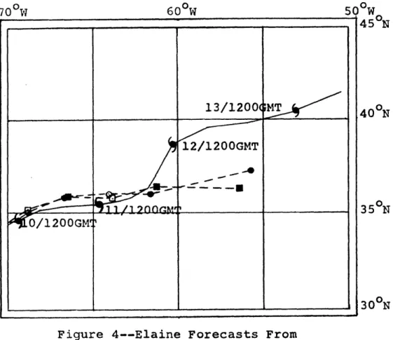
The two forecasts were for tropical storm Elaine, from initial data on September 10 and 11, 1974, at 1200 GMT. As previously noted, even these two cases still suffered from inadequate data coverage. On September 10, new bogus data could be determined for only 14 points, while the September 11 case provided revised data at only 9 points. The former case was
considered a good forecast and the latter was considered bad, at least at 48 hours. The original SANBAR forecast results as well as the revised forecast results are
listed in Table 8, and shown in Figures 4 and 5.
The September 10 case exhibits some improvement at 24 and 48 hours, but poorer results at 72 hours. The September 11 case shows virtually no change at any time. Elaine was a weak tropical storm that moved
generally ENE until September 12 at 00GMT when it abruptly moved almost northward for approximately 24 hours and
then returned to the ENE direction. Neither the
original nor the revised forecast was able to predict the northward turn causing the large errors.
The results of the Elaine cases are inconclusive regarding the value of the satellite winds in the initial analysis. The lack of data coverage is very evidently a prime factor. More work with better
documented cases is necessary to reliably evaluate the satellite data.
-33-TABLE 8
Forecast Results For Tropical Storm Elaine
Forecast (Date/Time) September 10, 1974/1200GMT Original Bogus Revised Bogus September 11, 1974/1200GMT Original Bogus Revised Bogus Position Error (NM) 24 Hr 48 Hr 72 Hr 105 100 67 237 36 299 105 265 106 264 ---~+- ----~~
-34-700W 600W 500W 45N 13/1200MMT 40N 12/1200GMT 35 N 111__/1200GM35 30
0
N
Figure 4--Elaine Forecasts FromSeptember 10, 1974, 1200GMT
--- 4 -- Best Track of Actual Storm
---4o---Forecast With Original Bogus ---- -- Forecast With Revised Bogus
For forecasts, closed symbols indicate 24, 48, and 72 Hr positions.
-35-70 W 60oW 50oW 45oN 13/1200GT 40
2/1200GMT
l/1200GMT 350N 10/1200GM 30N Figure 5--Elaine Forecasts FromSeptember 11, 1974,1200GMT
---
Best Track of Actual Storm ---- o--Forecast With Original Bogus---Forecast With Revised Bogus For forecasts, closed symbols
indicate 24, 48, and 72 Hr positions.
-36-ACKNOWLEDGEMENTS
Many people and organizations contributed much to the research and writing of this thesis, and I would like to acknowledge:
The USAF Air Force Institute of Technology for providing the opportunity for me to pursue this study at MIT,
Professor Frederick Sanders, my advisor, who gave inval-uable insight and assistance throughout the research and preparation of this study,
My wife, Cindy, for typing the many drafts and final manuscript and providing much needed moral support,
Professor E. N. Loranz who greatly aided the development of the regression analysis procedures,
Isabelle Kole for drafting some of the figures,
Mark Zimmer and the National Hurricane Center for out-standing personal and technical assistance in re-running the test cases,
L.F. Hubert and the National Environmental Satellite
Service for providing technical assistance and information, Paul Mulder and the National Center for Atmospheric
Research for assistance in obtaining data for the test cases,
and the
USAF Environmental Technical Applications Center for providing other data for this study.
- 4~
-37-This project was funded by the USAF Cambridge Research Laboratory.
-38-REFERENCES
1. Burpee, R.W., 1972: The origin and structure of Easterly Waves in the lower troposphere of
North Africa. J. Atmos. Sci., 29, No. , pp7 7-90. 2. Gaertner, J.P., 1973: Investigation of forecast
errors of the SANBAR hurricane track model. SM thesis, Dept. of Meteorology, Mass. Inst. of Tech., unpublished.
3. Hubert, L.F., 1975: Private communication. 4. Hubert, L.F. and L.F. Whitney, Jr., 1971: Wind
estimation from geostationary-satellite pictures. Mon. Wea. Rev., 99, pp665-672.
5. Lorenz, E.N., 1975: Class notes, Dept. of Met-eorology, Mass. Inst. of Tech., unpublished. 6. Newell, R.E., J.W. Kidson, D.G. Vincent, G.J. Boer.
The General Circulation of the Tropical Atmo--sphere and Interactions with Extratropical Lat-itudes. Vol. 1 & 2, Mass. Inst. of Tech. Press,
1973 & 1974.
7. Pike, A.C., 1975: Private communication.
8. Sanders, F., 1959: The application of pressure-averaged flow to the problem of hurricane dis-placement. AFCRC-TR-59-254, AD 212263.
9. Sanders, F., 1970: Dynamic forecasting of tropical storm tracks. Trans. New York Acad. Sci.,
Series 11, 32, pp495-508.
10. Sanders, F. and R.W. Burpee, 1968: Experiments in barotropic hurricane track forecasting. J. Appl. Meteor., 7, pp313-323.
11. Sanders, F., A.C. Pike, and J.P. Gaertner, 1975: A barotropic model for operational prediction of tracks of tropical storms. J. Appl. Meteor., 14, No. 3, pp265-280.
-39-APPENDIX A
Determination Of Satellite Cloud-Motion Vectors
Satellite cloud-motion vectors are derived from analysis of successive photographs of cloud patterns. Individual cloud elements, or target clouds, are
iden-tified and tracked to determine their motion and esti-mate the wind field in which they are embedded. More
than one level of cloud can often be detected and
identified to obtain wind estimates at that cloud level. The height resolution can be determined from different cloud motions over the same area, infrared measurements of cloud top temperatures, and subjective observations of cloud type, brightness and texture. The estimated heights of the clouds are subject to some uncertainties and are generally classified simply as low, middle, or high cloud levels.
Hubert and Whitney (1971) determined the heights of the lower and upper cloud layers from comparison of the motion of the target clouds to hodographs of nearby rawinsondes. The LBF or "level of best fit" was deter-mined from the assumption that the minimum velocity
difference between the balloon wind the cloud-motion vec-tor occurred at cloud level. They found that the
low-level clouds correspond best to the 3000 to 5000-ft. layer and the high-level clouds correspond to the 30,000 ft. level.
Currently, the level of the cloud is obtained by measuring the temperature of the cloud top with infrared sensors and then comparing this temperature to the vertical
temperature profile obtained from the National Meteorologi-cal Center (NMC) forecast model. TropiMeteorologi-cal cumulus are
-40-very prevalent in the forecast area and are easily
identified as low clouds. The low clouds are generally assigned to the 900 mb level over the oceans although the 850 mb level is also often used. The upper cloud levels correspond well to 200 mb between 00 and 300N and to 300 mb north of 300N. Middle level clouds are sometimes identified and are generally representative of the 500 mb level. (Hubert, 1975)
Satellite cloud-motion vectors are used operation-ally in some forecast models. Under certain assumptions, these winds are used at more than one level. For this reason, NMC provides the low level winds at both the
850 and 700 mb levels, the mid-level at 500 mb, and the high level at 300, 250, and 200 mb levels.
-41-APPENDIX B Analysis Of Data
The rawinsonde winds are inputs to a computer analysis that develops the mean wind and statistical quantities necessary to form the equation sets. The winds are first resolved into u and v components and then each component is treated separately to develop u and v regression equation sets. The 10 levels of rawinsonde data determine the mean wind components. The mean wind components and the components of the 850 500- and 250-mb winds are then used to compute variances and covariances of the quatities needed to solve for the coefficients of the regression equations.
The mean wind is formed in the computer analysis subject to certain assumptions and constraints. The
flow in the troposphere is pressure averaged over the 10 mandatory levels. Lower and upper level mean winds are formed from the lower four and upper six levels respectively. The mean wind is then determined by
linear averaging of the two. The sounding is discarded if certain conditions are met concerning missing data: 1) if more than two lower or three upper level winds are missing, 2) if both 1000 and 850 mb winds are
missing, or 3) if any four consecutive winds are missing. If the sounding is not discarded, missing winds are
linearly interpolated before any computations are performed.
-42-APPENDIX C
Data Stratification
The 20 station sample produced a total of 27,421 soundings for computation after screening by the com-puter analysis. Six geographical and three time
stratifications were considered as shown in Table 1. The geographical stratifications were based primarily on natural groupings of the 20 stations by
their locations. Set 1 covers the western Atlantic, the Gulf of Mexico, and the Caribbean. Set 2 covers the east central Pacific from the California coast to Midway Island. Set 4 covers the southwestern Pacific
islands. Sets 3, 5, and 6 are combinations of sets 1, 2 and 4.
Originally, it was hoped that the data could be stratified by latitude and by hemisphere to determine if there was any justification for such groupings. The availability of data, however, did not allow such
stratification. Sets 1 and 2 are in the western hemi-sphere and north of 170N while Set 4 is in the eastern hemisphere but south of 19oN with 6 of the 8 stations between 00 and 100N. Stratification by geographical
location also stratifies by latitude and hemisphere at the same time causing uncertainty as to what factors might actually contribute to any difference in the
equation sets. Sets 3 and 5 were used to check if any effects of location could be detected. Set 6, which included all 20 stations as one data sample, combined all of the possible geographical effects to produce a set of equations for general use in the latitude zone from which the stations were chosen. The selection process used for the analysis would seem to restrict
-43-data area as is intended for tropical storm prediction. The effects of topography would have to be considered over land areas and would require the use of inland stations to include these effects in the development of new regression equations.
Stratification according to time was considered to investigate any seasonal variation between summer and early fall. The five month period was divided
into June, July, August, and September, October to form two sets of regression equations. The geographical stratifications were maintained, and three sets were considered for time stratification. Set 1 seemed to be the most likely set to exhibit time dependence due to the location of its stations.near mid latitudes. Set 4 is located deep in the tropics and primarily
south of 10ON. This set should exhibit little, if any, seasonal change. Set 6 was used to combine all the geographic factors and consider time dependence on the entire sample. Set 2 was not considered due to its small size and location north of the preferred storm
-44-APPENDIX D
Details of Linear Regression Analysis
Let y be the predictand (the component of the mean wind in either the u or v direction)
Let xi be the predictors (1, 2, or 3 predictors as required)
Define xo = 1 for ease of notation
Let ai be the coefficients of the predictors xi with
ao being the constant term in the equation Define e as the residual error after prediction
A A
Define y as the predicted value of y so that y= y + e ( ) denotes an average over the sample: x =
4;
N = sample size
Therefore: y =
Zaixi
+ ei=o
A-so that y = aixi where k can = 1, 2, or 3. I=0
The ai are chosen to minimize e2, the mean square error, so that e e = 0 _ ai Now: ~2 = 2 2 ebe = +exi = 0 ai b ai
Application of the above forms a set of k + 1 equations:
ao + xjla + 0xkak = .. y
xl ao + xal + *..xlxkak = xlY
xkao + xkxla1 + .. xak = xkY
The elimination of ao from the equations reduces the set to k equations:
lili-
-45-x' al + *... Xx k ak = xjly
xkxl al + ... xk ak = xkY
Where the prime ( )' denotes the departure from average, (xi - T) X, x= x is the variance of xi, and xixk
is the covariance of xi and xk*
2 2 -2
xi = (xi
-
i) (xi - Xi)0 I
xlxk
= (x - 3 )(xk -X) = (ixk - x xk)The variances and covariances are evaluated from the computer analysis of the rawinsonde data and are used to determine the a 's.
a is determineg by: a =y a .x
The equations for the 1, 2, and 3 predictor sets are shown in Table D1
The reduction of variance, r2 is defined by:
k
2 e2 aixiY
r =1- =Z t
y y
From this expression, e2 can be determined by: e = (1 - r ) y
The reduction of variance equations used in this report are shown in Table D2.
The standard deviation is defined as the square root of the variance:
S= 2
The root mean square error is the square root of e2. rms error =V
-46-TABLE Dl 3 Predictor - 2 + *, , , , X1 al + XlX2 a2 + XlX3 a3 = xlY XlX2 al + x2a 2 + x2x 3 a3 = x2Y xlx3 a1 + x2x3 a2 + x 3 a3 = x3 a = y - alx1 - a2x2 a3x 3
y = a + alx1 + a2x2 + a3x 3 2 Predictor 12 , x1 al + X1 x3 a3 = xlY S3'2 ' XlX3 al + x3 a3 = x3Y a = y - alx I - a3x3 y= a + al 1 + 1 Predictor a) 850 mb----xlY a 1 x1 a = y - alx1 A y = a + alx1 b) 250 mb S 3 x3y a3 = x3 a = y - a3x3 A y = a0 + a3x3 (850 mb, 500 mb, 250 mb) (850 mb, 250 mb) a3x3 x = 850 mb wind component x2 500 mb wind component x3 = 250 mb wind component
-47-TABLE D2 3 Predictor 2 r = (850 mb, 500 mb, 250 mb) I I I I I I alxly + a2x2y + a3x 3Y '2 y 2 Predictor alxly + a3x3Y '2 y (850 mb, 250 mb) 1 Predictor a) 850 mb 1 3 2 alxlY r-1 '2 y b) 250 mb 2 a3x 3Y r3 2 '2
Y
~ (.___ I__ULI_~~I~
-48-APPENDIX E
Evaluation of The Prediction Sets
The three-predictor equation closely approximates the mean tropospheric flow as discussed in Section 5. Unfortunately, the operational usefulness of this
equation is limited since the mid-level satellite wind is rarely available. The most operationally useful equation is the two-predictor, since two levels of
data are routinely available. Given good data coverage at these levels, the two-predictor equation can provide reasonable values of the mean flow.
The one-predictor equation can be operationally useful in cases of good coverage at one level but little
or no coverage at the other. The accuracy of the single-predictor equation is less than for the two-single-predictor, but still somewhat better than climatology. The rms errors from the one-predictor equation can be compared
to the standard deviations of the mean wind in Table 6. The 250-mb equation sets show lower rms errors than the
850-mb sets and, therefore, provide more prediction skill. The increase in rms error due to the use of satellite data in the rawinsonde-derived equations is discussed in Appendix G.
-49-APPENDIX F
Effects of Sampling On The Regression Analysis
The regression equations have shown reasonable skill in predicting the wind in the dependent data
sample from which they were derived. The question then arises as to the ability of the equations to predict the mean wind in a new independent data sample. The
equations must be evaluated to determine their reliability. As previously defined, the reduction of variance in the dependent sample is
r2 =1- 1)
y2
The reduction of variance will decrease in a new data sample due to the process of sampling. The amount of this decrease can be characterized by a new quantity called the expected reduction of variance,p . The expected reduction of variance is an estimate of how well the equations will perform on a new data sample.
is dependent on the number of predictors in the equations, the original reduction of variance, and the number of independent observations in the dependent sample. The expected reduction of variance is then:
S 2 2MN 22)
= r - (1 - r ) 2)
1 3
(N + 1)(N - M -1)
where r2 is the original reduction of variance, M is the number of predictors, and N is the adjusted sample size.
The quantity N can be equal to N, the original sample size, but in many cases it is less than N. This is due to the fact that N is the number of independent observations in the sample while N is simply the total
-50-number of observations. If the observations are chosen completely at random such that all are independent of the others, N = N. In this study, however, the observations are chosen as consecutive rawinsonde soundings on 153 consecutive days for 5 consecutive years. This formu-lation suggests that there is a dependency of one obser-vation on another implying that N is less than N. The amount that N is less than N is not an exact figure, but can be estimated.
The initial assumption for determining N is that the winds in one year will not be dependent on any other year so that each year can be considered to be independent. The five month time span per year is 153 days. Since
two soundings are generally made per day, the initial
one year sample is 306 observations per station. However, the two (or more) daily soundings must be assumed to be dependent causing a reduction of the sample size by one-half leaving 153 potential observations.
Burpee (1972) determined that African waves in the lower troposphere have periods of 3-5 days. Based on this and other considerations of tropical flow patterns, it seems reasonable to assume that an independent obser-vation should be obtained at least in every 5-7 days. Assuming the time scale to be 7 days gives 21 independent
observations per year per station. Therefore, the value of N will be 105 observations per station for the 5 year sample. The values of N and are tabulated in Table F1 for each of the geographical stratifications.
The expected loss in skill of prediction is negligible due to the small number of predictors and the large number of independent observations.
-51-TABLE F1
Expected Reduction of Variance A) Set No. of Stns. N N 1 8 11682 840 2 4 5594 420 3 12 17276 1260 4 8 10145 840 5 12 15739 1260 6 20 27421 2100 B) Set Il r2 u v u v 1 3 0.9739 0.9528 0.9737 0.9525 2 3 0.9647 0.9601 0.9642 0.9598 3 3 0.9714 0.9562 0.9713 0.9560 4 3 0.9240 0.8855 0.9235 0.8845 5 3 0.9588 0.9337 0.9586 0.9334 6 3 0.9684 0.9445 0.9683 0.9443 1 2 0.9144 0.8508 0.9140 0.8501 2 2 0.8723 0.8781 0.8711 0.8769 3 2 0.9043 0.8591 0.9040 0.8587 4 2 0.7701 0.6967 0.7690 0.6953 5 2 0.8613 0.8047 0.8609 0.8041 6 2 0.8929 0.8478 0.8927 0.8475 1 1/850 0.4301 0.3377 0.4287 0.3361 2 1 0.2658 0.2511 0.2623 0.2475 3 1 0.3625 0.2826 0.3615 0.2815 4 1 0.2422 0.2367 0.2404 0.2349 5 1 0.1837 0.2270 0.1824 0.2258 6 1 0.3053 0.2777 0.3046 0.2770
-52-TABLE F1 B) (cont'd) Set M rV u v u v 1 1/250 0.6911 0.5952 0.6904 0.5942 2 1 0.6824 0.7680 0.6809 0.7669 3 1 0.6757 0.6564 0.6752 0.6559 4 1 0.2774 0.4179 0.2157 0.4165 5 1 0.5864 0.6306 0.5857 0.6300 6 1 0.,6325 0.6098 0.6321 0.6094
-53-APPENDIX G
Analysis Of Satellite Data Error
Inherent in the determination of satellite cloud-motion vectors is the possibility of "error" when they are compared to the actual flow at the
level as defined by rawinsonde data. This error is more accurately a difference between the data sources
and is possibly due to a difference in the scale of observed motion. The satellite winds are determined from cloud motions over broad areas and generally represent the large scale flow. They do, however, suffer from errors in measurement and from height uncertainty as detailed by Hubert and Whitney (1971). The rawinsonde data, as a whole, represent the large
scale flow, but individual stations can often be indluenced by small scale fluctuations.
This difference or error is not simply a question of accuracy, but is a question of the applicability of the rawinsonde-derived equation to satellite data. As discussed in Section 6, the satellite wind can be
considered as the sum of the rawinsonde wind and some effective error as:
X. = (x.i + ei )
The variances and covariances for satellite data are then:
'2 '2 1 ' '2
X.i xi + 2xiei + ei
1 1 1 1 1
X.X. = xix j + xiej + xjei + eiej (1)
XiY = xiy + eiy
where y is the actual mean wind. Since the errors have
~LIYLI~-(I~-
-54-been assumed to be uncorrelated with the wind and with each other, the covariances involving the errors will be equal to zero and equations 1 reduce to:
x 2 X'2 +12 X = x. +e.
X. = x x. (2)
Xiy = xiy
Revised regression equation analysis for the satellite data produces new coefficients ai for the two-predictor equations as shown:
(x.y )(x. + e. ) (xx .)(x3y
.'2 '2 '2 '2 ' 3 2
(xi + e )(x + e
)
- (x2 '2 '2 '2
where (x. + e. ) and (x. + e. ) are sirmulated sat-ellite winds at the two levels. The new reduction
of variance is defined by equation 3 in Section 6. The effects of the satellite error on the two-predictor equation are shown in Section 6, Table 7.
Analysis of the one-predictor equations produces similar results. Table G1 shows the effect of the
satellite error for set 1 (Western Atlantic, Caribbean, Gulf of Mexico) and set 4 (Southwestern Pacific) and for their individual stations. The increase in the rms error varies from about 1% to about 20% for assumed realistic values of the error and can be compared to the standard deviation of the mean wind. Some varia-bility can be seen in the rms errors within each
stratification set. The stations are arranged in the table by decreasing latitude with the most northerly first within each set. Less variability is seen in
-55-low latitudes as is to be expected. The single-pre-dictor equations show little improvement over clima-tology in most cases, but the 250-mb sets do exhibit modest skill at the higher latitudes. Operational
testing of the one-predictor equations is necessary to actually determine their prediction skill.
-56-TABbL G1
Effects of Satellite Error on One-Predictor Equations
u Component '2 '2 e. = 0.25x2 i i 850 mb Rawinsonde Satellite 250 mb Rawinsonde Satellite Int. Index. No. 72304 78016 72240 72211 72250 72202 76644 78526 Set 1 91245 91217 91413 91366 91334 91408 91376 91348 Set 4 IT
r2
() 40 42 28 34 22 34 22 34 43 35 49 39 20 30 46 18 15 24 9.8 8.7 9.7 9.1 9.4 8.4 6,1 6.2 8.8 7.3 5.5 4.7 5.5 5.1 4.8 5.2 5.1 6.0 10.4 9.2 10.1 9.6 9.7 8.8 6.3 6.5 9.5 7.7 6.0 5.0 5.7 5.3 5.2 5.3 5.2 6.2T2
12.7 11.3 11.4 11.2 10,7 10.4 6.9 7.6 11.7 9.1 7.7 6.1 6.2 6.1 6.6 5.8 5.5 6.9 70 63 77 73 82 72 65 55 69 58 23 18 26 21 17 24 28 28 7.0 6.9 5.5 5.8 4.6 5.5 4.1 5.1 6.5 5.9 6.8 5.5 5.3 5.4 6.0 5.0 4.7 5.8 8.4 8.0 7.1 7.2 6.3 6.7 4.8 5.7 7.8 6.6 7.0 5.6 5.5 5.6 6.1 5.2 4.9 6.1 r2 ("I"~' -.-XI--~-(I.I ~.LIIXI -IWlti
111
I I
-57-APPENDIX H
Selection And Analysis of Study Cases
The 53 SANBAR forecasts were evaluated for position errors at 24, 48, and 72 hours with the "best track" storm locations as supplied by NHC. The best track is the official track of the storm as determined from all observations. The position error was simply calculated as the vector difference between the SANTBAR forecast position and the best track position at the same time. Good and bad SANBAR forecasts were initially identified for study. The criteria for judging good from bad is that a good forecast should have a position error of less than 75, 150, and 300 NM at 24, 48, and 72 hours respectively, as discussed by Sanders et al (1975). Every "good" forecast does not meet every one of these position error values, but these criteria are generally useful for evaluation.
The analysis procedure first involved plotting the data on low-level and high-level charts. Streamline analysis was used to determine the flow patterns where possible at each level. From these patterns, two levels of data could be obtained for a bogus point and the mean wind calculated from the regression equations. The data for each bogus point had to be interpolated and was, therefore, subject to errors whose magnitudes depended largely on the quality of the data coverage. The error could be almost zero in areas of good coverage and quite large in poor coverage areas. The value of the inter-polation error is difficult to evaluate, but it must be considered, in some manner.