HAL Id: hal-01419768
https://hal.archives-ouvertes.fr/hal-01419768
Submitted on 3 Jun 2020
HAL is a multi-disciplinary open access archive for the deposit and dissemination of sci-entific research documents, whether they are pub-lished or not. The documents may come from teaching and research institutions in France or
L’archive ouverte pluridisciplinaire HAL, est destinée au dépôt et à la diffusion de documents scientifiques de niveau recherche, publiés ou non, émanant des établissements d’enseignement et de recherche français ou étrangers, des laboratoires
The impact of pollution abatement investments on
production technology: new insights from frontier
analysis
Jean Pierre Huiban, Camille Mastromarco, Antonio Musolesi, Michel Simioni
To cite this version:
Jean Pierre Huiban, Camille Mastromarco, Antonio Musolesi, Michel Simioni. The impact of pollution abatement investments on production technology: new insights from frontier analysis. 10. Journées de recherches en sciences sociales (JRSS), Société Française d’Economie Rurale (SFER). FRA.; Centre de Coopération Internationale en Recherche Agronomique pour le Développement (CIRAD). FRA.; Institut National de la Recherche Agronomique (INRA). FRA., Dec 2016, Paris, France. 29 p. �hal-01419768�
The impact of pollution abatement
investments on production technology: new
insights from frontier analysis
Jean Pierre HUIBAN
INRA-ALISS,
65 bd de Brandebourg, 94205 Ivry Cedex, France
Camilla MASTROMARCO
Dipartimento di Scienze dell’Economia, University of Salento, Ecotekne, via per Monteroni, 73100 Lecce, Italy,
email: camilla.mastromarco@unisalento.it
Antonio MUSOLESI
Department of Economics and Management (DEM), University of Ferrara, and SEEDS
Via Voltapaletto 11, 44100 Ferrara, Italy email: antonio.musolesi@unife.it
Michel SIMIONI
INRA, UMR 1110 MOISA
2, place Pierre Viala - Bt. 26 - 34 060 Montpellier Cedex 2, France
The impact of pollution abatement investments on
production technology: new insights from frontier
analysis
Abstract
This paper estimates the impact of pollution abatement investments on the production technology of firms by pursuing two new directions. First, we take advantage of recent econometric developments in productivity and efficiency analysis and compare the results obtained with two complementary approaches: parametric stochastic frontier analysis and conditional nonparametric frontier analysis. Second, we focus not only on the average e↵ect but also on its heterogeneity across firms and over time and search for potential nonlinearities. We provide new results suggesting that such an e↵ect is heterogeneous both within firms and over time and indicating that the e↵ect of pollution abatement investments on the production process is not monotonic. These results have relevant implications both for modeling and for the purposes of advice on environmentally friendly policy.
Keywords: Pollution abatement investments, technology, stochastic frontier analysis, conditional nonparametric frontier analysis, full and partial order frontiers, generalized product kernels, infinite order cross-validated local polynomial regression.
1
Introduction
Pollution clearly appears to be an undesirable output of production. Because producing cleanly is more expensive than polluting, environmental regulation may be necessary in order to incite firms to make investments devoted to pollution reduction and to pursue a sustainable process of economic development. A standard view among economists is that environmental regulation aiming to reduce pollution is a detrimental factor for firms’ competitiveness and productivity (Jorgenson and Wilcoxen, 1990). Since the early 1990s, however, this view has been challenged by numerous economists. In particular, Porter (1991) and Porter and Van der Linde (1995) argued that more stringent but properly designed environmental regulations do not inevitably hamper firms’ competitiveness but could enhance it. This new paradigm has become known as the ‘Porter hypothesis’. Since then, such a hypothesis has received much attention. It was initially criticized for its lack of an underlying theory (Palmer et al., 1995) and for being incon-sistent with the empirical evidence (Ja↵e et al., 1995), while today a more solid theory exists (Andr´e, 2015) but also mixed empirical evidence, so that the validity of the Porter hypothesis continues to be one of the most contentious issues in the debate regarding environmental reg-ulation. All this suggests that “further research is clearly needed in this area” (Ambec et al., 2013, p. 10).
This paper aims to contribute to the literature by pursuing two new directions.
First, within a methodological perspective, we aim to assess the e↵ect of pollution abatement investments on the production technology of firms by adopting methods that have been recently developed by the econometric literature on productivity and efficiency analysis and that leave room for the consideration of external factors of production. External variables are generally defined as variables that cannot, at least totally, be controlled by the producer but may have an influence in the production process (B˘adin et al., 2012). The available measures of firms’ e↵orts to reduce pollution, such as pollution abatement investments, can be seen as these kinds of variables, as they are expected to be stimulated by environmental regulation and, at the same time, to have some kind of e↵ect on the production technology of firms.
A second novel aspect of this paper is its modeling and policy-oriented perspective. Specif-ically, we focus not only on the average e↵ect but also on its variability across firms and over time and search for potential nonlinearities. These aspects have been recognized as extremely relevant by the theoretical literature and have important implications, but until now, they have been neglected by the existing empirical literature. Indeed, as already pointed out by previous works (Ambec et al., 2013), the controversy over the Porter hypothesis centers on the likelihood that the regulatory costs may be fully o↵set or not. The critics say that although some anec-dotal empirical evidence in the direction suggested by Porter could be found, a complete o↵set should be seen as the exception. Porter and van der Linde also admit that such a complete o↵set does not always occur. Moreover, the linearity and monotonicity of the relation can also be questioned, as “it is not reasonable to assume that the e↵ect of environmental regulation is monotonic” (Andr´e, 2015, p. 29) since it could be that taking advantage of regulation will become more difficult if the stringency of environmental regulation will increase too much.
In order to model pollution abatement investments as external factors of production and to address the above issues, two complementary approaches are adopted in this paper: parametric stochastic frontier analysis (SFA) and conditional nonparametric frontier analysis (CNFA). They present relative advantages and drawbacks; comparing their results may be useful to provide a more nuanced and thorough picture of the e↵ect of pollution abatement investments on the production technology of firms. It may be also important to provide more robust results. SFA has the relative advantage of having a well-developed statistical theory which allows for statistical inference. Therefore, using SFA we can test alternative specifications as well as di↵erent hypotheses on efficiency. We can focus our attention on input elasticities, on their heterogeneity across firms and on all the other estimated parameters of the production frontier and get information on scale economies, efficiency, etc. Conversely, CNFA has the relative advantage over SFA that it does not make any assumptions, either about specific parametric functional form for the production frontier or about distributional assumptions on the noise and inefficiency component, and may be useful to detect complex nonlinear relations. At the same time, however, this flexibility comes at a price since CNFA does not allow the estimation of some key elements of production econometrics (such as input elasticities, scale economies, etc.) and inference is less straightforward than in SFA.
More specifically, concerning SFA, the most common approaches in the literature model the impact of external factors either on the structure of the technology or on technical efficiency (Coelli et al., 1999). We follow and extend these trends and consider alternative models to include pollution abatement investments in the production process and then use the Vuong (1989) test in order to select the most likely one. When switching to CNFA, we use a two-step approach similar to Mastromarco and Simar (2015) where at the first stage conditional non-parametric efficiency measures are obtained and are used as exploratory tools (Cazals et al., 2002; Daraio and Simar, 2005; B˘adin et al., 2012) and, at the second stage they are regressed nonparametrically over pollution abatement capital. We follow recent advances in nonparamet-ric kernel regression and depart from previous works since, at the second stage, we avoid ad hoc determination of the local polynomial order by using the ‘infinite order cross-validated local polynomial regression approach’ recently proposed by Hall and Racine (2015). This methods allows – via delete-one cross-validation – the joint determination of the polynomial order and bandwidth and this can have a relevant impact on the quality of the resulting approximation. In summary, to the best of our knowledge, this is the first work estimating the e↵ect of pollution abatement investments on the production technology of firms using methods that model pollution abatement investments as external factors of production and, at the same time, focusing on some aspects – such as heterogeneity and nonlinearity – that have been shown to be relevant by the theoretical literature and have important implications for firms and society as a whole in terms of advice on environmentally friendly policy.
The present paper is organized as follows. Section 2 gives a brief review of the related literature. Section 3 presents the econometric methodologies while the description of the data
2
Literature
In this section, we present the general ideas and the di↵erent versions of the Porter hypoth-esis. We also briefly review the theoretical literature, specifically highlighting the economic mechanisms allowing for a possible positive relation between pollution abatement investments and firm-level productivity. For a more exhaustive discussion on both theory and empirics, the reader is referred to the recent surveys by Ambec et al. (2013) and Andr´e (2015).
According to a standard view among economists, at least until the 1990s, pollution abate-ment e↵ort due to environabate-mental regulation may be beneficial in terms of environabate-mental per-formance but would negatively a↵ect firms’ economic perper-formances since it forces them to allocate the production inputs to pollution reduction, pushing them away from optimal pro-duction choices and thus inducing technological and allocative inefficiency.
Since the early 1990s, however, this traditional paradigm has been challenged by what has become known as the ‘Porter hypothesis’ (Porter, 1991; Porter and Van der Linde, 1995). Porter and Van der Linde (1995, p. 98) suggest that “Strict environmental regulation can trigger innovation (broadly defined) that may partially or more than fully o↵set the traditional costs of regulation”.
Since then, the Porter hypothesis has attracted a great deal of attention, theoretically as well as empirically. However, a difficulty that arises when addressing such a hypothesis is clarifying its interpretation, as the Porter hypothesis is not a hypothesis in a statistical sense but it represents a general idea illustrated with real-life examples and, at least in its original formulation, lacked an underlying theory (Palmer et al., 1995). Ja↵e and Palmer (1997) help in the interpretation of the Porter hypothesis by distinguishing between the ‘weak’, ‘narrow’ and ‘strong’ versions of such a hypothesis. According to the weak version, environmental regulation may stimulate innovation, while the narrow version argues that certain types of environmental regulation, but not all, spur innovation. This idea that regulation can stimulate innovation is based on the concept of induced innovation and goes back to Hicks (1932). It is generally accepted and has been validated by many previous studies, even those specifically about envi-ronmental regulation. The core of the controversy lies in the strong version, which argues that in many cases this innovation more than o↵sets the regulatory costs, ultimately enhancing firms’ competitiveness and economic performances. From a theoretical point of view, after some initial criticisms (Palmer et al., 1995), the literature has provided alternative explana-tions supporting the strong version, such as firms’ behaviors departing from the assumption of profit maximization (Ambec and Barla, 2007), market failure (Andr´e et al., 2009), organization failure (Ambec and Barla, 2002), and knowledge spillovers (Mohr, 2002).
It should also be noted that while Porter and van der Linde claim that firms become “more competitive”, the concept of competitiveness is quite general and allows for alternative measurements. As a consequence, the above-mentioned theoretical works have considered alternatives measures of competitiveness such as cost reduction, increased profits or higher market shares. At the same time, however, empirical research has focused on the estimation of production functions or productivity equations. Somewhat more closely related to this
empirical literature, Mohr (2002) emphasizes productivity increases and justifies the Porter hypothesis by adopting a general equilibrium model where a key role is played by external economies and in particular the nature of knowledge as a public good. According to such a model, firms’ output benefits from knowledge spillovers. The amount of this common knowledge is equal to the cumulative production experience of all firms using the same technology. Thus, a specific firm will switch to a new (greener) technology only if enough other firms have done it first. This is because, even if new and greener technology will be, ceteris paribus, more productive, at least initially there is much more accumulated experience in the old technology than in the new one and, as a consequence, the productivity of the new technology will be lower than that of the old one. Environmental regulation can thus solve the coordination problem, inciting firms to adopt the greener technology, which will increase the global stock of knowledge of the new technology, and ultimately lead to an improvement in the level of productivity of those firms.
3
Methodology
There is a huge body of empirical literature testing the strong version of the Porter hypothesis, but it provides rather mixed empirical evidence (Ambec et al., 2013). This literature focuses on the estimation of production functions or productivity equations augmented with some measures of pollution abatement e↵orts. We follow the stream of the literature using a direct measure of the expenditures or investments engaged by the firms (see e.g., Shadbegian et al., 2005) and estimate value-added production frontiers where the pollution abatement e↵orts are measured with the stock of capital devoted to pollution reduction (a detailed description of the data is in section 4).
The methodology we use departs from previous studies in that it is inspired by recent developments in the econometric literature on productivity and efficiency analysis that allow the consideration of external factors of production. SFA and CNFA provide useful frameworks for dealing with this issue. This section shows how these two approaches can be used to model the impact of pollution abatement capital on the production process.
3.1
Stochastic frontier analysis
The most common approaches in the SFA literature model the impact of external factors either on the structure of the technology or on technical efficiency (Kumbhakar and Lovell, 2000). We follow and extend these trends and consider two alternative models to include pollution abatement capital in the production process.
Input model
In a first model, which we label as the input model, we assume that pollution abatement cap-ital influences the production process itself, or, put di↵erently, enters the production function, F (.), as an additional factor of production in the stochastic production frontier model
Yit = F (t, Kit, Lit, Zit)⌧itwit. (1)
The output of a firm i at time t, Yit, is thus assumed to be determined not only by the levels
of usual inputs, i.e. labor input, Lit, and physical capital, Kit, but also by pollution abatement
capital, Zit. The time trend t captures technological change over time and we do not assume
Hicks-neutrality. The wit, which are assumed to be independent and identically distributed
random errors, capture the stochastic nature of the production frontier. ⌧it denotes technical
efficiency with 0 < ⌧it 1 and ⌧it = 1 when the firm produces on the frontier.
The stochastic production frontier model in Eq. (1) is parameterized using a translog specification achieving local flexibility (also called Diewert flexibility, see e.g., Fuss et al., 1978) and outperforming other Diewert-flexible forms (Guilkey et al., 1983):
yit = ↵ + ⌧t + kkit+ llit+ zzit+ ⌧ t2 2 + k k2 it 2 + l l2 it 2 + z z2 it 2 + + ⌧ ktkit+ ⌧ ltlit+ ⌧ ztzit+ klkitlit+ kzkitzit+ lzlitzit uit+ vit (2)
where lower case letters indicate variables in natural logs, i.e. yit = ln(Yit), and so on. It is
worth noting that this specification is more general than the one chosen by Coelli et al. (1999) which restricts the e↵ect of external factors only to the shape of the technology by imposing
z = ⌧ z = kz = lz = 0 in Eq. (2). Put di↵erently, we do not exclude the case where
pollution abatement capital a↵ects the technology of the firms as an input under the control of the firm manager choosing the optimal level of pollution abatement investments given some external constraints (such as environmental regulation) and within its maximization program. The error term in Eq. (2) is composed of two components, the two-sided noise component vit = ln(wit) and the non-negative technical inefficiency component uit = ln(⌧it). The noise
component, vit, is assumed to be independently and identically distributed as N (0, v2) and
distributed independently of uit. The technical inefficiency component, uit, is assumed to be
time-varying. Two di↵erent assumptions about the distribution of this component can then be made. First, we can assume that the technical inefficiency component is of the multiplicative form:
uit = `(t, T )⇥ ui
where ui is distributed as N (µ, u2) truncated at zero and `(t, T ) is written as
`(t, T ) = exp(
T
X
t=2
where dt denote year dummies.1 Hereafter we will refer to this specification as multiplicative.
A second specification for the inefficiency component, which we label as additive, builds on Battese and Coelli (1995) and Coelli et al. (1999) with uit distributed as N (µit, u2) truncated
at zero and µit = µ + T X t=2 tdt (4)
The two specifications of the technical inefficiency component di↵er in the way they model time-varying inefficiency. In the multiplicative specification, the underlying truncated nor-mal variable ui is scaled by the exponential function of time. The inefficiency component in
this specification varies in a systematic way with respect to time. Greene (2005) defines this specification of the inefficiency component as “time-dependent” rather than as time-variant. The other inefficiency specification is a pooled model where the time variation of inefficiency depends on the way time a↵ects the mean of the truncated distributed variable uit.
Efficiency model
In the input model, pollution abatement capital is assumed to influence production directly, by a↵ecting the structure of the production frontier relative to which the efficiency of firms is estimated. An alternative model associating variation in efficiency with variation in pollution abatement capital can be also considered. In this model, which is labeled as the efficiency model, Eq. (1) becomes
Yit = F (t, Kit, Lit)⌧it(Zit)wit. (5)
where we assume now that pollution abatement capital, Zit, influences production, Yit,
indi-rectly, through its e↵ect on technical efficiency, ⌧it. The stochastic production frontier model
in Eq. (5) is parameterized using a flexible translog specification as yit = ↵ + ⌧t + kkit+ llit+ ⌧ t2 2 + k k2 it 2 + l l2 it 2 + ⌧ ktkit+ ⌧ ltlit+ klkitlit uit+ vit (6) Here too, the error term in Eq. (6) is composed of two components, the two-sided noise component vit= ln(wit) and the non-negative technical inefficiency component uit= ln(⌧it).
We assume again that the noise component, vit, is independently and identically distributed as
N (0, 2
v) and distributed independently of uit. Two alternative specifications of the distribution
of the technical inefficiency component, uit, are considered, a multiplicative one and an additive
one, as for the input model. But now, the multiplicative form of the inefficiency component in the multiplicative model becomes
uit= `(t, T, Zit)⇥ ui,
1By construction, a constant term in Eq. (3) capturing the e↵ect of the first year cannot be identified
where ui is distributed as N (µ, u2) truncated at zero and `(t, T, Zit) is written as `(t, T, Zit) = exp( T X t=2 tdt+ ✓Zit), (7)
Meanwhile, the assumptions in the additive model become uit distributed as N (µit, u2)
trun-cated at zero and
µit = µ + T
X
t=2
tdt+ ✓Zit (8)
To sum up, we have four parametric models: input model with multiplicative inefficiency component, input model with additive inefficiency component, efficiency model with multi-plicative inefficiency component, and efficiency model with additive inefficiency component. These four models are estimated by maximum likelihood. Since they are non nested, in order to choose the preferred specification, we perform the modified likelihood-ratio test proposed by Vuong (1989) to compare non-nested models.
3.2
Conditional Nonparametric Frontier Analysis
The parametric approach allows the estimation of some key parameters of production econo-metrics, such as elasticities, scale economies, etc. However, even if a flexible form is used to represent the production technology, such an approach might su↵er from misspecification problems due to imposing a specific functional form on the production process and assuming known statistical distributions on the errors terms.2 The use of nonparametric methods serves
to relax these restrictive parametric assumptions, even if these methods do not allow the es-timation of parameters for economic interpretation. Moreover, using recent developments in nonparametric frontier literature (Cazals et al., 2002; Daraio and Simar, 2005 and 2007; B˘adin et al., 2012, Mastromarco and Simar, 2015), it is possible to disentangle the potential e↵ects of conditioning variables (in our case, pollution abatement capital) to identify e↵ects on the boundary (the shape of the frontier) and e↵ects on the distribution of the inefficiencies in a full nonparametric setup.
First step: Exploratory tools
We follow Cazals et al. (2002), Daraio and Simar (2005, 2007) and, mainly, Mastromarco and Simar (2015) who introduce the time dimension into the conditional frontier model. The production process generates random variables (X, Y, Z) in an appropriate probability space, where X 2 Rp+denotes the vector of inputs, Y 2 Rq+denotes the vector of outputs, and Z 2 Rr+
denotes the vector of variables describing external factors, i.e. factors that may influence the production process and the efficiency pattern (in our case, pollution abatement capital and time). As suggested by Mastromarco and Simar (2015), time can be handled as a Z variable.
2For instance, Guilkey et al. (1983) have shown that the translog approximation outperforms other
Diewert-flexible forms such as the generalized Leontief and the generalized Cobb-Douglas, but also provides a reliable approximation only if the complexity of the underlying technology is not too high.
For each time period t, the attainable set z ⇢ Rp+q
+ is defined as the support of the
conditional probability3
HX,Y|Z(x, y|z) = Prob (X x, Y y| Z = z) .
The function HX,Y|Z(x, y|z) is simply the probability for a firm operating at level (x, y) to be
dominated by firms facing the same external conditions z. Accordingly, the conditional output-oriented technical efficiency of a production plan (x, y)2 z, i.e. facing external conditions z,
can be defined as (Daraio and Simar, 2005)
⌧ (x, y|z) = sup {⌧|(x, ⌧y) 2 z} = sup{⌧|SY|X,Z(⌧ y|x, z) > 0}.
where SY|X,Z(y|x, z) = Prob(Y y|X x, Z = z) is the (nonstandard) conditional survival
function of Y, nonstandard because the condition on X x and not X = x.4
We also calculate partial frontiers, introduced by Daouia and Simar (2007), enabling us to obtain results that are robust to some extreme observations. Conditional (unconditional) output-oriented robust order-↵ quantile efficiency measures are defined for any ↵ 2 (0, 1) as:5
⌧↵(x, y|z) = sup{⌧|SY|X,Z(⌧ y|x, z) > 1 ↵}
As stated in B˘adin et al. (2012), the e↵ect of external factors on the shape of the fron-tier can be investigated by considering the ratios of conditional (⌧ (x, y|z)) to unconditional (⌧ (x, y)) efficiency measures, which are measures relative to the full frontier of respectively, the conditional and the unconditional attainable production sets:
RO(x, y|z) =
⌧ (x, y|z)
⌧ (x, y) . (9)
By construction, RO(x, y|z) 1, whatever the triplet (x, y, z). In turn, the e↵ect of
exter-nal factors on the distribution of technical efficiencies can be investigated using the ratios of conditional to unconditional output-oriented robust order-↵ quantile efficiency measures for 3From now on, we use capital letters for random variables and lowercase letters for the values these random
variables take.
4Let H
X,Y(x, y) denote the unconditional probability of being dominated. Then we have
HX,Y (x, y) =
Z
Z
HX,Y|Z(x, y|z) fZ(z)dz
having support , the unconditional attainable production set which is defined as = Sz2Z z. It is clear
that, by construction, Z ⇢ . Unconditional output-oriented technical efficiency of a production plan (x, y),
can then be defined as
⌧ (x, y) = sup{⌧|(x, ⌧y) 2 } = sup{⌧|SY|X(⌧ y|x) > 0},
where SY|X(y|x) = Prob(Y y|X x) is the unconditional survival function of Y given that X x. Here
too, it is clear that, by construction, ⌧ (x, y|z) ⌧(x, y).
5The unconditional measures are: ⌧
di↵erent values of ↵, i.e
RO,↵(x, y|z) =
⌧↵(x, y|z)
⌧↵(x, y)
. (10)
Here the ratios RO,↵(x, y|z) can be either 1 or 1. But as ↵ ! 1, RO,↵(x, y|z) ! RO(x, y|z)
For the output orientation, when the ratios (9) are globally increasing with an external factor, this indicates a favorable e↵ect on the production process, and the external factor can be considered as a freely available input. Indeed, the value of ⌧ (x, y|z) is much smaller (greater efficiency) than ⌧ (x, y) for small values of the factor than for large values of it. In our case with Z as pollution abatement capital, this may be explained by the fact that firms facing small values of the external factor do not take advantage of the favorable environment, and when the value of the external factor increases, they benefit more and more from the environment. On the contrary, when the ratios (9) are globally decreasing with the external factor, there is an unfavorable e↵ect of this factor on the production process. The external factor is then acting as an unavoidable output. In this situation ⌧ (x, y|z) will be much smaller than ⌧(x, y) for large values of the external factor.
As explained in B˘adin et al. (2012), the full frontier ratios (9) indicate only the e↵ects of external factors on the shape of the frontier, whereas with the partial frontier ratios (10), these e↵ects may combine e↵ects on the shape of the frontier and e↵ects on the conditional distri-bution of the inefficiencies. For our purpose of analyzing the impact of Z on the distridistri-bution of efficiencies, we are interested in the median, by choosing ↵ = 0.50. If the e↵ect on partial frontier ratios is similar to the one shown with the ratios with full frontier, we can conclude that we have a shift of the frontier while keeping the same distribution of the efficiencies when the external factor changes. If the e↵ect with the median (↵ = 0.5) is greater than for the full frontier, this indicates that in addition to an e↵ect on the shape of the frontier, we also have an e↵ect on the distribution of the efficiencies.6
Nevertheless, the conclusions of the analysis of ratios should be taken with caution and regarded only as exploratory. In fact, they are valid if the choice of inputs is independent of the external factors. If not, the analysis of the ratios as a function of the external factors should be conducted for fixed levels of the inputs. The interpretations given above as to the impact of the external factors, which depends on the shape of the relation between the ratios and the factors, remain valid, but for a fixed vector of inputs.
Second step: Nonparametric regression of the conditional efficiency scores To go further into the analysis of the impact of external factors, B˘adin et al. (2012) propose to analyze the average behavior of ⌧ (x, y|z) as a function of z, in order to capture the main e↵ect of the external factors on these conditional measures. We thus regress, in the second stage, the conditional efficiency scores ⌧ (x, y|z) on pollution abatement capital and time. This is motivated by the fact that the so-called ‘separability condition’ discussed in Simar and Wilson (2007) likely does not hold. Indeed, under such a condition, neither time nor pollution abatement capital influences the shape of the attainable set. But this appears very restrictive 6The full frontier corresponds to an extreme quantile, i.e. the maximum achievable output. See Figure 10,
and an unlikely event since if technical change occurs, the frontier of the attainable set will change with time. In such a case, as suggested by B˘adin et al. (2012), in the second stage it is meaningful to analyze the average behavior of the conditional efficiency scores ⌧ (x, y|z) - rather than the unconditional ones ⌧ (x, y) - as a function of the external factors. Here too, the conditional efficiency scores ⌧ (x, y|z) may also vary with both z and x. But now, we want to capture the marginal e↵ect of Z on the efficiency scores, so it is legitimate to analyze the regression model E (⌧(x, y|z)|Z = z) as a function of z. Therefore, we focus attention on the following nonparametric regression function:
⌧ (x, y|z) = m(z) + "
where m(.) is un unknown smooth function to be estimated and " is the usual error term such that E("|Z = z) = 0.
To estimate this model, we follow recent advances in nonparametric kernel regression and depart from the above-mentioned works which estimate location-scale regression models with the local constant approach, for two reasons. First and most important, we use the ‘infi-nite order cross-validated local polynomial regression approach’ recently proposed by Hall and Racine (2015) rather than adopting the local constant approach most often used in previous works. The method proposed by Hall and Racine (2015) instead allows – via delete-one cross-validation – the joint determination of the polynomial order and bandwidth, avoiding the ad hoc determination of the polynomial order, which is the standard practice in applied works. As also stressed by Hall and Racine (2015), the order of the polynomial can have a relevant im-pact on the quality of the resulting approximation, while the appropriate order will in general depend on the underlying and unknown DGP. Such a method allows improvements in both finite sample efficiency and in the rate of convergence, which for some common DGPs, is equal to the parametric rate for the Oracle estimator, O(n 1/2). Second, we do not use the
location-scale regression model, i.e. when the error term can be expressed as " = (z)". While in some cases it could be of interest to adopt this model, in our specific case we do not focus on the scale e↵ect, V (⌧(x, y|z)|Z = z), whereas the location e↵ect, E (⌧(x, y|z)|Z = z), is of primary interest. If one wants to estimate the variance function 2(z) in the location-scale model, one
simply needs to regress nonparametrically the square of the residuals on the external factors.
4
Data
We build a new and rich firm-level panel data set concerning the French food processing indus-tries and covering a relatively long period (1993-2007). The French food processing industry is particularly relevant for such a kind of analysis because it is one of the most polluting sectors with respect to several indicators - especially concerning the e↵ects of total final consumption of the produced goods (European Environmental Agency, 2006) - and it is one of the sectors
investing more in pollution abatement.7 It is finally also relevant in terms of size, representing
a large proportion of manufacturing in France (about 550,000 employees in 2011, i.e. 18% of manufacturing employment).
Data for the French food processing industries on pollution abatement investments are collected annually in a survey conducted by the French ministry of Agriculture, called Enquˆete Annuelle sur les D´epenses pour Prot´eger l’Environnement (ANTIPOL), since the early 1990s. To our knowledge, this paper represents the first attempt to use this survey for academic purposes. The ANTIPOL survey provides information on pollution abatement investments defined as “the purchase of buildings, land, machinery or equipment to limit the pollution generated by production activity and internal activities or the purchase of external services improving the knowledge to reduce pollution”. Next, the pollution abatement capital stock at firm level is built using the perpetual inventory method with a depreciation rate of 15%. This is a standard rate adopted in the literature for investments in pollution abatement (Aiken et al., 2009).
The Enquˆete Annuelle d’Entreprise (EAE) is an annual firm-level survey covering almost all firms with 20 or more employees, conducted by the French National Institute for Statistics. This survey provides a measurement for output, i.e. value-added, deflated by its annual industry price index, and for the usual inputs, i.e. labor measured by the number of employees expressed in annual full-time equivalent workers, and capital measured by the amount of fixed assets, deflated by the annual price index for capital goods.
The two data sets are merged, finally resulting in an unbalanced panel data set composed of 8391 observations and 1130 firms covering the period 1993-2007. Table 1 presents some descriptive statistics for the variables used to estimate the production function: value added, labor (number of workers), physical capital stock, and pollution abatement capital stock.8
This table shows that average pollution abatement capital stock is about one-fiftieth of av-erage physical capital stock. Also note that a fraction of firms has never invested to reduce pollution, the corresponding stock of capital presents many zeros (18.21% of the total number of observations), but all the explanatory variables are expressed in logarithms when using a translog specification. To include all the observations for the variable Z, we follow Battese (1997), and set z ⌘ ln (Z + D) where D = 1 if Z = 0, and D = 0 if Z > 0, as explanatory variable instead of ln (Z) which is not defined when D = 1. Battese (1997) also introduces the variable D as a shifter of the constant term. As we introduce sectoral dummies to capture unobserved heterogeneity across sectors, we do not introduce the dummy D. Indeed, sectoral dummies can capture the e↵ect of omitted variables that explain the heterogeneity of pollu-tion abatement investment behaviors across sectors, making the dummy D redundant. The same definition, z ⌘ ln (Z + D), is also adopted when implementing conditional nonparametric frontier estimation.
7In 2007, the food processing industry was found to be the third biggest spender on pollution abatement
investments in France (e167 million), only exceeded by the energy (e437 million) and chemicals, rubbers and plastics (e204 million) industries.
Table 1
5
Results
5.1
SFA
Model selection
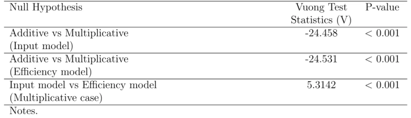
The four parametric models proposed above are estimated and then the Vuong (1989) test is performed to select the most likely one.9 Results are reported in Table 2. The Vuong test
indicates that the multiplicative specification of efficiency is preferred to the additive one, for both the input and efficiency models. It also shows that the input model is preferred to the efficiency model when comparing them in the multiplicative case. Consequently, we select the multiplicative input model as the most likely one at the end of the model selection procedure.
Table 2
We then proceed to test the null hypothesis that pollution abatement capital a↵ects only the shape of the production technology as in the Coelli et al. (1999) model, i.e. we test the null hypothesis that z = ⌧ z = kz = lz = 0 in Eq. (2).The likelihood ratio test statistics
whose value is 18.616 with a p-value equal to 0.001, allow us to reject such a hypothesis. Estimation of the preferred model
The estimated values of the parameters of the preferred model, i.e. the multiplicative input model, serve to compute the output elasticities with respect to K, L and Z and are noted as "Y,K, "Y,L and "Y,Z. While the average values of "Y,K, "Y,L and "Y,Z are equal to 0.255, 0.780 and
0.018, respectively, we mainly focus our attention on the estimation of the underlying density functions. They are of interest in order to have information about the variability across firms and over time of such elasticities. In particular, we estimate the conditional densities of the above elasticities conditioned on time. Time being an ordered variable, we adopt the approach by Hall et al. (2004) which uses generalized product kernels to deal with mixed data and cross-validation to choose the smoothing parameters. We use a second order Gaussian kernel for the continuous variable and a Li and Racine’s (2007) kernel for the ordered conditioning variable time. According to Hall et al. (2004), cross-validated smoothing parameters will behave in such a way that the smoothing parameters for the irrelevant conditioning variables converge in probability to the upper extremities of their respective ranges, i.e. 1 for the ordered Li and Racine’s (2007) kernel. Irrelevant conditioning variables are thus smoothed out. At the other extreme, when such a smoothing parameter is zero, the generalized estimator collapses to the standard frequency estimator.
Figure 1
Figure 1 reveals that the distributions of "Y,K and "Y,L are clearly unimodal. Conversely,
and very interestingly, it can be observed that the density of "Y,Z is bimodal and appears
to be a mixture of two underlying densities, a first one with a negative mode and a second one with a positive mode. Overall, about 80% of the firms have a positive elasticity. This result has two interpretations. First, it suggests that the traditional view about the e↵ect of environmental regulation on productivity and the Porter hypothesis may coexist. Second, it reinforces the view that the firms’ e↵orts to reduce pollution do not always positively a↵ect the firms’ performances, but they do in many cases, as also stressed by Ambec et al. (2013). Concerning the time evolution of the distributions of such elasticities, Figure 1 also reveals that the distribution of "Y,Z has clearly evolved over time - the smoothing parameter for time is 0.44
- and shows a positive shift. Indeed, while at the beginning of the period, a relevant fraction of the firms are characterized by a negative elasticity, at the end of it, almost all the firms have a positive elasticity. Also note that this result could be considered as consistent with the theoretical paper by Mohr (2002) since it is observed that the annual share of firms investing in pollution abatement increased over the period (see Appendix). According to this model, firms benefit from knowledge spillovers where the amount of knowledge equals the cumulative experience of all firms using the same technology so that a specific firm will switch to a new (greener) technology only if enough other firms have done so first.
Next, we focus on the elasticities of substitution. While for a concave production function with two inputs, the elasticity of substitution among them is always positive (inputs are substi-tutes), in three- (or more) input production functions, as a result of the all possible interactions among inputs, an increase in one input may be associated with an increase in the use of an-other input, to maintain the same level of output. In such a case, these two inputs are called complements (see e.g. Chambers, 1988). To measure the degree of substitutability between any two inputs, a widely adopted measure is the Allen partial elasticity of substitution, which is defined by: ij = PT t=1iXifi XiXj Fij F ,
where Xidenotes input i, fi ⌘ @f/@Xi, F is the determinant of the bordered Hessian of the
pro-duction function whose elements are 0, fi and fij ⌘ @2f /@Xi@Xi. Fij is the associated cofactor
of fij. If f (X) is concave, a factor of production cannot be a complement for all other factors
in terms of the Allen elasticity. This is appealing since it appears to be intuitively consistent with the two-input case where factors are always substitutes. Figure 2 shows the estimated conditional densities of the Allen elasticities of substitution conditional on time. labor and capital, and labor and pollution abatement capital are always substitutes, with median values of the elasticities equal to 1.65 and 1.62 respectively. Their densities are tightened around a single mode and right skewed. The estimated density of Allen elasticity of substitution between capital and pollution abatement capital is also unimodal but is negatively skewed, suggesting that capital and pollution abatement capital are substitutes for most firms (the median value of
the elasticity is equal to 0.16) but at the same time they are complements for other firms. Con-cerning the time patterns of the distributions of these elasticities, the smoothing parameter for time ranges between 0.67 and 0.72, suggesting that appreciable changes over time occurred in the overall distribution of the three partial Allen elasticities. At the same time, however, while the median value of the elasticities of substitution labor-capital and labor-pollution abatement capital does not vary significantly over time, the substitutability between capital and pollution abatement increases constantly over the period, its median varying from -0.10 in 1993 to 0.32 in 2007.
Figure 2
Finally, note that natural outcomes of the estimation of the multiplicative input model are the time-varying efficiency scores. They can be computed as exp ( E (uit|"i1, . . . , "iTi)) where
"it = vit uit, using an extension of the Jondrow et al. (1982) estimator of efficiency score
to the input model with multiplicative efficiency. At the same time, however, they are not a central interest of this paper and detailed results on these scores are available upon request.
5.2
CNFA
To complement the previous analysis, we conduct the CNFA analysis detailed above. CNFA may serve to detect a possibly complex nonlinear e↵ect of pollution abatement capital on the production process. Moreover, CNFA also permits us to understand whether external factors a↵ect both the shape of the frontier and the distribution of efficiencies.
As a first step, we investigate the ratios of conditional and unconditional efficiency measures for full and partial frontiers. The conditional DEA estimates are computed with the localizing procedure described in Mastromarco and Simar (2015) and optimal bandwidths have been selected by least squares cross-validation. Figure 3 shows the ratios from a marginal point of view, i.e. as a marginal function of pollution abatement capital.10 The full frontier ratios (top
panel) show a nonlinear e↵ect of pollution abatement capital on the shape of the frontier. This nonlinear e↵ect takes the shape of an inverted U relation suggesting the existence of a positive e↵ect on the shape of the frontier when pollution abatement capital increases at low values of capital and a decreasing e↵ect for large values of capital. In order to check the robustness of our result and to inspect whether some extreme observations would hide an e↵ect, we calculated the ratios for partial frontiers with ↵ = 0.99, and obtained very similar results, which are available upon request. According to B˘adin et al. (2012), the full frontier ratios also provide useful information on the ‘separability condition’, which in this case, seems clearly to be violated, because our external variable - pollution abatement capital - is a↵ecting the boundary of the production set (shifts of the production frontier).
panel) displays a slightly favorable e↵ect of pollution abatement capital. We observe a very flat relation for most of the range of pollution abatement capital which becomes positive for the highest values of such a variable.11
These results seem to confirm our previous parametric ones that pollution abatement capital acts more as production factor, a↵ecting the shape of the frontier, than a productivity factor, influencing the inefficiency. Thus pollution abatement capital impacts mainly on the shift of the boundary and less on the distribution of inefficiencies. Hence, from this evidence, pollution abatement capital appears to weakly a↵ect efficiency (technological catch-up) and play a more important role in accelerating technological change (shifts in the frontier).
Figure 3
Given that the separability assumption is not verified, in order to analyze and isolate the e↵ect of pollution abatement capital and time on the distribution of efficiencies, it is necessary to move to the second-step nonparametric regression using conditional efficiency scores as a dependent variable.12 Consequently, in the second step, as suggested by B˘adin et al. (2012)
and Mastromarco and Simar (2015), we regress the log of conditional efficiency scores as a function of pollution abatement capital (in logs) and time.13 We use the method proposed by
Hall and Racine (2015) to estimate the location e↵ect. Bernstein polynomials are employed (note that a Bernstein polynomial is also known as a Bezier curve) and the generalized product kernel is obtained as a product of a second order Gaussian kernel for the continuous predictor, pollution abatement capital, and a Li and Racine’s (2007) kernel for the ordered variable time. The delete-one cross validation procedure provides a first order local polynomial for pollution abatement capital and bandwidths equal to 0.223 and 0.172, for pollution abatement capital and time, respectively. According to Hall et al. (2007), these results indicate that both regressors are relevant.
Figure 4
Figure 4 shows that pollution abatement capital has a nonlinear e↵ect on the conditional efficiencies. Indeed, for very low levels of pollution abatement capital, the conditional effi-ciency scores log⌧ (x, y|z) - pollution abatement capital relation is quite flat, suggesting that a minimum level of capital devoted to pollution abatement is necessary to produce an e↵ect. Then, after reaching a threshold, this relation is no longer flat but roughly shows an inverted U pattern. We clearly see negative and then positive average e↵ects of pollution abatement capital on conditional efficiency (a decrease of log⌧ (x, y|z) indicates an increase in efficiencies, the optimum being zero).
11The results are very stable to changes in the quantile. Detailed results obtained for other values of ↵ are
available upon request.
12Indeed, if the separability condition is not verified, unconditional efficiency scores do not provide useful
information since they ignore the heterogeneity introduced by the external variables on the attainable sets of values for (X, Y ).
The e↵ect of pollution abatement capital seems much more important than the e↵ect of time, except for small values of pollution abatement capital. This finding suggests that pol-lution abatement capital needs to reach a certain level to drive efficiency externalities. The e↵ect of time is less important for large values of pollution abatement capital, supporting the hypothesis of decreasing adjustment costs and time delays.
The bottom two panels of Figure 4 exhibit the marginal view from the perspective of time and abatement pollution capital.14 This evidence, combined with the previous ones, highlights
the nonlinear influence of pollution abatement capital on efficiency. The time shows a slight positive e↵ect on efficiency revealing a very slow technological catching-up process among the firms under analysis.
In summary, these results complement the previous ones obtained using parametric fron-tiers. Indeed, on the one hand, comparing these nonparametric findings with the elasticity obtained from the preferred parametric input model, provides confirmation of the existence of a heterogeneous e↵ect of pollution abatement capital on the shape of the frontier but also suggests a particular shape (inverted U) without imposing a specific functional form. On the other hand, when we estimated the parametric efficiency model in equation (7) we found that pollution abatement capital has a positive - but low in magnitude and not significant - e↵ect on efficiency. This possibly was the result of the imposed parametric specification and distribution assumptions on the error terms, since the second-step nonparametric regression performed in this section indicates a rather complex nonlinear relation. To our knowledge, this is the first econometric work showing the existence of a non-monotonic e↵ect as suggested, for instance, by Andr´e (2015).
6
Conclusions
This paper estimates the impact of pollution abatement investments on the production tech-nology of firms, using a novel and rich panel data set covering the French food processing industries over the period 1993-2007. It aims to contribute to the literature by pursuing two new directions. First, with respect to a methodological perspective, we take advantage of recent developments in productivity and efficiency analysis that allow the consideration of external factors of production. Specifically, we compare the results obtained with two com-plementary approaches: parametric stochastic frontier analysis and conditional nonparametric frontier analysis. These methods present relative advantages and drawbacks and comparing their results may be useful to provide a more robust and thorough picture of the e↵ect of pol-lution abatement investments on the production technology of firms. A second novel aspect of this paper is its modeling and policy-oriented perspective, since we pay attention not only to the average e↵ect but also on its variability across firms and over time, and search for eventual nonlinearities. These aspects have been recognized as extremely relevant by the theoretical literature and have important implications for firms and society as a whole in terms of advice
on environmentally friendly policy.
We provide new results suggesting that the e↵ect of pollution abatement capital on the shape of the production frontier is heterogeneous both within firms and over time, and reinforcing the view that firms’ e↵orts to reduce pollution do not always positively a↵ect their performances, but do in some cases. We have also documented that the substitutability between pollution abatement capital and physical capital increases constantly over the period. Finally, when switching to a fully nonparametric framework, relevant complementary results are provided. In particular, using this approach it was possible to uncover a nonlinear and non-monotonic e↵ect of pollution abatement capital, both on the shape of the frontier and on the conditional efficiencies. These results have relevant implications both for modeling purposes and in terms of policy advice.
References
[1] Aiken, D. V., Fare, R., Grosskopf, S. and Pasurka C. A.. (2009) Pollution Abatement and Productivity Growth: Evidence from Germany, Japan, the Netherlands, and the United States. Environmental and Resource Economics, 44, 11-28.
[2] Ambec, S., Cohen, M. A., Stewart, E. and Lanoie, P. (2013) The Porter Hypothesis at 20: Can Environmental Regulation Enhance Innovation and Competitiveness?. Review of Environmental Economics and Policy, 7, 2-22.
[3] Ambec, S. and Barla, P. (2006) Can Environmental Regulations be Good for Business? An Assessment of the Porter Hypothesis. Energy Studies Review, 14, 42-62.
[4] Ambec, S. and Barla, P. (2002) A Theoretical Foundation to the Porter Hypothesis. Eco-nomics Letters, 3, 355-360.
[5] Andr´e, F.J., Gonz´alez, P. and Porteiro, N. (2002) Strategic Quality Competition and the Porter Hypothesis. Journal of Environmental Economics and Management, 57, 182-194. [6] Andr´e, F.J. (2015) Strategic E↵ects and the Porter Hypothesis. MPRA Paper 62237,
University Library of Munich, Germany.
[7] B˘adin, L., C., Daraio, L., Simar, L. (2010) Optimal bandwidth selection for conditional efficiency measures: A data-driven approach. European Journal of Operational Research, 201, 633-640.
[8] B˘adin, L., C., Daraio, L., Simar, L. (2012) How to measure the impact of environmental factors in a nonparametric production model. European Journal of Operational Research 223, 818-833
[9] Battese, G. E. (1997) A Note on the Estimation of Cobb-Douglas Production Function when Some Explanatory Variables have Zeros. Journal of Agricultural Economics, 48, 250-252.
[10] Battese, G. E., and Coelli, T. J. (1992) Frontier Production Functions, Technical Efficiency and Panel Data: With Application to Paddy Farmers in India. Journal of Productivity Analysis, 3, 153-69.
[11] Battese, G.E., and Coelli, T.J. (1995) A Model for Technical Efficiency E↵ects in a Stochas-tic Frontier Production Function for Panel Data. Empirical Economics, 20, 325-32. [12] Cazals, C., Florens, J.-P., and Simar, L.(2002) Nonparametric frontier estimation: a robust
approach. Journal of Econometrics, 106, 1-25.
[13] Chambers, R.G. (1988). Applied Production Analysis. A Dual Approach. Cambridge Uni-versity Press, Cambridge.
[14] Coelli, T., Perelman, S., Romano, E. (1999) Accounting for Environmental Influences in Stochastic Frontier Models: with Application to International Airlines. Journal of Pro-ductivity Analysis, 11, 251-273.
[15] Daouia, A. and Simar, L (2007) Nonparametric Efficiency Analysis: A Multivariate Con-ditional Quantile Approach. Journal of Econometrics, 140, 375-400.
[16] Daraio, C. and Simar, L. (2005) Introducing environmental variables in nonparametric frontier models: a probabilistic approach. Journal of Productivity Analysis, 24, 93-121. [17] Daraio, C., Simar, L (2007). Advanced Robust and Nonparametric Methods in Efficiency
Analysis. Springer, New-York
[18] Fried, H. O., C. A. K. Lovell, S. S. Schmidt and Yaisawarng, S. (2002) Accounting for environmental e↵ects and statistical noise in Data Envelopment Analysis. Journal of Pro-ductivity Analysis 17, 157–174.
[19] Fuss, M., D. McFadden and Mundlak, Y. (1978) A survey of functional forms in the eco-nomic analyses of production. in M.Fuss and D.McFadden (eds), Production Ecoeco-nomics: A Dual Approach to Theory and Applications, North-Holland, Amsterdam.
[20] Greene, W. (2005) Reconsidering Heterogeneity in Panel Data Estimators of the Stochastic Frontier Model. Journal of Econometrics, 126, 269-303.
[21] Guilkey, D.K., Lovell, C.A.K. and Sickles, R.C. (1983) A Comparison of the Performance of Three Flexible Functional Forms. International Economic Review, 24, 591-616.
[23] Hall, P., Li, Q., and Racine, J.S. (2007) Nonparametric estimation of regression functions in the presence of irrelevant regressors. The Review of Economics and Statistics, 89, 784-789.
[24] Hall, P.G., and Racine, J.S. (2015) Infinite Order Cross-validated Local Polynomial Re-gression. Journal of Econometrics, 185, 510-525.
[25] Hicks, J. R. (1932). The theory of wages, 1st ed. London, Macmillan.
[26] Ja↵e,A.B., and Palmer, K. (1997) Environmental Regulation And Innovation: A Panel Data Study. Review of Economics and Statistics, 79, 610-619.
[27] Ja↵e, A.B., Peterson, S.R., Portney, P.R. and Stavins, R.N. (1995) Environmental Regu-lation and the Competitiveness of U.S. Manufacturing: What Does the Evidence Tell Us?. Journal of Economic Literature, 23, 132-163
[28] Jondrow, J., Lovell, C.A.K., Materov, I. and Schmidt, P. (1982), On the Estimation of Technical Inefficiency in the Stochastic Frontier Production Function Model. Journal of Econometrics 19, 233-238.
[29] Jorgenson, D. W. and P. J. Wilcoxen, (1990) Environmental Regulation and U.S. Economic Growth. The RAND Journal of Economics, 21, 314-340.
[30] Kallis, G., Butler, D. (2001) The EU water framework directive: measures and implica-tions. Water Policy, 3, 125–142.
[31] Lanoie, P., J. Laurent-Lucchetti, N. Johnstone and Ambec, S. (2011) Environmental Pol-icy, Innovation and Performance: New Insights on the Porter Hypothesis. Journal of Economics & Management Strategy, 20, 803-842.
[32] Li, Q., and Racine, J.S. (2007). Nonparametric Econometrics: Theory and Practice, Princeton University Press.
[33] Mastromarco, C. and Simar, L. (2015) E↵ect of FDI and Time on Catching up: New Insights from a Conditional Nonparametric Frontier Analysis. Journal of Applied Econo-metrics, 30, 826-847.
[34] Mohr, R.D. (2002) Technical Change, External Economies, and the Porter Hypothesis . Journal of Environmental Economics and Management, 43, 158-168.
[35] Palmer, K.W., Oates, W.E. and Portney, P.R. (1995) Tightening Environmental Standards The Benefit-Cost or the No-Cost Paradigm. Journal of Economic Perspectives, 9, 119-132. [36] Porter, M. S. (1991) America’s Green Strategy. Scientific American, 264, 168.
[37] Porter, M. S. and Van der Linde, C. (1995) Toward a New Conception of the Environment-Competitiveness Relationship. Journal of Economic Perspectives, 9, 97-118.
[38] Vuong, Q (1989) Likelihood Ratio Tests for Model Selection and Non-Nested Hypotheses. Econometrica 57, 307-333.
Appendix: Description of the panel
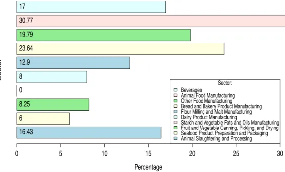
Let us first focus on firms’ pollution abatement investments. The share of firms investing in pollution abatement activities at least one year during the period 1993-2007, for the 1130 firms constituting the unbalanced panel, is equal to 85.22%. Figure 5 reports the percentages of non investing firms in the di↵erent sectors of the French food processing industry.15 Pollution
abatement investment behaviours are di↵erent across sectors. All firms invested at least once in the highly polluting starch and vegetable fats and oils manufacturing sector, while only two thirds of firms did so in the beverage sector.
Figure 5
Consider now the trends in pollution abatement investments. The annual share of investors increases from 51.95% in 1993 to 65.16% in 2007, as shown in Figure 6. Such an increase is mostly due to a level shift that occurred from 2000 to 2001 when the share of firms investing to reduce pollution moved from 53.06% to 68.82%. This is likely due to stricter environmental constraints. In 2000, indeed, the European Union promulgated a relevant directive, i.e., the EU water framework directive, aiming to achieve a good status for all waters and introducing new standards for managing Europe’s waters (see e.g., Kallis and Butler, 2001). The treatment of waste water is one of the most important fields for pollution abatements, concerning on average more than 50% of the total pollution abatement investments of the French food industry. At the same time, when focusing only on the firms investing in pollution abatements, it can be noted that the average amount of investments decreases from 320.932 KEuros in 1993 to 247.261 KEuros in 2007 and that this decrease occurred in the 2000s, as shown in Figure 6.
Figure 6
15The French food industry can be broken down into 10 sectors when the NACE classification at the 3-digit
Table 1: Summary statistics
Variable Label Mean Std. dev. Value-Added (K Euros) Y 27605.71 52847.71 labor (Number of workers) L 418.03 534.38 Capital stock (K Euros) K 47756.40 104830.80 Pollution Abatement Capital stock (K Euros) Z 980.53 2575.60
Table 2: Model selection results
Null Hypothesis Vuong Test P-value Statistics (V)
Additive vs Multiplicative -24.458 < 0.001 (Input model)
Additive vs Multiplicative -24.531 < 0.001 (Efficiency model)
Input model vs Efficiency model 5.3142 < 0.001 (Multiplicative case)
Notes.
The Vuong statistic, V , is asymptotically distributed as standard normal distribution. If V > 1.96, then the first model is favored at 5% significance level.
If V < 1.96, then the second model is favored at 5% significance level. Otherwise, for 1.96 V 1.96, neither model is preferred.
time 1995 2000 2005 E_K 0.1 0.2 0.3 0.4 Conditional Density 2 4 6 Capital time 1995 2000 2005 E_L 0.6 0.7 0.8 0.9 1.0 Conditional Density 2 4 6 Labour time 1995 2000 2005 E_Z −0.02 0.00 0.02 0.04 Conditional Density 20 40 60
Pollution abatement capital
time 1995 2000 2005 E_LK 1.6 1.8 2.0 Conditional Density 1 2 3 4 Labour vs Capital time 1995 2000 2005 E_ZL 1.4 1.6 1.8 2.0 2.2 Conditional Density 0.5 1.0 1.5 2.0 2.5 3.0
Labour vs Pollution Abatement Capital
time 1995 2000 2005 E_ZK −1.5 −1.0 −0.5 0.0 0.5 Conditional Density 0.5 1.0
Capital vs Pollution Abatement Capital
0 2 4 6 8 10
0.6
0.9
Marginal effect of pollution abatement capital on the ratios R
O(x,y | z)
Pollution abatement capital (in logs)
ratio
0 2 4 6 8 10
0.7
1.0
1.3
Marginal effect of pollution abatement capital on the ratios R
O , 0.5(x,y | z)
Pollution abatement capital (in logs)
ratio
Figure 3: The top panel represents the full ratio bRO(x, y|z) as a marginal function of pollution
abatement capital (in logs). The bottom panel is the ratio bRO,↵(x, y|z, t) for ↵ = 0.5, so for the
0 2 4 6 8 10 0.00 0.05 0.10 0.15 0.20 0.25 0.30 0.35 0 2 4 6 8 10 12 14 16 Z time E [ τ (x,y|z)] 0 2 4 6 8 0.00 0.05 0.10 0.15 0.20 Z Conditional Mean 1 2 3 4 5 6 7 8 9 10 11 12 13 14 15 0.00 0.05 0.10 0.15 0.20 as.ordered(time) Conditional Mean
Sector: Beverages
Animal Food Manufacturing Other Food Manufacturing
Bread and Bakery Product Manufacturing Flour Milling and Malt Manufacturing Dairy Product Manufacturing
Starch and Vegetable Fats and Oils Manufacturing Fruit and Vegetable Canning, Pickling, and Drying Seafood Product Preparation and Packaging Animal Slaughtering and Processing
Percentage Sector 0 5 10 15 20 25 30 16.43 6 8.25 0 8 12.9 23.64 19.79 30.77 17
Figure 5: Percentages of pollution abatement non investing firms in food processing industry sectors 1994 1996 1998 2000 2002 2004 2006 40 50 60 70 80
Annual share of firms investing in pollution abatement
year Ann ual share 1994 1996 1998 2000 2002 2004 2006 200 250 300 350 400
Annual average investment in pollution abatement (KEuros)
year
Av
er
age in
vestment


![[PDF] Tutoriel Générale de Microsoft Word 2007 | Cours informatique](data:image/gif;base64,R0lGODlhAQABAIAAAP///wAAACH5BAEAAAAALAAAAAABAAEAAAICRAEAOw==)