An alternative to the Kutta condition
for high frequency, separated flows
by
Alexandros Gioulekas
Dipl.Eng., National Technical University of Athens, 1985 S.M., Massachusetts Institute of Technology, 1987
Submitted to the Department of Aeronautics and Astronautics
in partial fulfillment of the requirements for the degree of
Doctor of Philosophy
at theMassachusetts Institute of Technology
May, 1992@1992, Alexandros Gioulekas
The author hereby grants to M.I.T. permission to reproduce and to distribute copies of this document in whole or in part.
Signature of Author N
May, 1992 Certified by
Certified by Prof. James E. McCune Thesis Supervisor
Certified by
,C/rtf
b
Prof. Alan Epstein
SThesis Committee Member Certified by
ri yProf. Manuel Martines-Sanches Thesis Committee Member Accepted by
.
/
A~rO
Prof. Harold Y. WachmanMASSACHUSETTS INSTITUTE Chairman, Departmental Graduate Committee OF TEP•Mni nr
JUN
0
5 1992
An alternative to the Kutta condition for high frequency, separated flows
by
Alexandros Gioulekas Submitted to the Department of
Aeronautics and Astronautics in partial fulfillment of the requirements for the Degree of
Doctor of Philosophy
Abstract
An alternative to the Kutta condition for determining the circulation around a bluff airfoil in unsteady, separated flow is presented. For such flows, there is a need for a practical criterion which would avoid the detailed boundary layer calculations and would predict the time evolution of the airfoil circulation based on the external potential flow only.
This criterion would play for unsteady, separated flows the role that the Kutta condition plays for flows past thin airfoils. It turns out to be a criterion for predicting the location and movement of the "separation points", because they determine the net vorticity flux shed into the wake and thus the rate of change of the airfoil circulation.
The laminar, two-dimensional flow about a bluff airfoil at angle of attack, when the external flow oscillates at a high reduced frequency is considered.
At high frequencies, the vorticity generated as the wall resists the imposed unsteadi-ness is confined to a thin layer near the blade surface ("Stokes layer") and its contri-bution to the displacement thickness is proportional to an inverse power of the reduced frequency and thus small. Outside this region, the unsteady part of the boundary layer velocity is approximately the external potential oscillation. Based on this observation and following C.C. Lin, the boundary layer velocity can be divided into two coupled velocity distributions, one predominantly oscillatory ("Stokes velocity") and another predominantly steady ("Prandtl velocity"). The main contributor to the displacement thickness is the latter. Therefore, separation, identified by a dramatic increase in the displacement thickness, can be located by calculating the evolution of the "Prandtl velocity"and finding where the latter bifurcates.
(arising through the coupling of the "Prandtl" to the "Stokes" flow by the no-slip condition on the wall and Reynolds-stress terms in the momentum equation), lead to a criterion for unsteady separation that uses as only inputs parameters of the external flow and avoids a detailed boundary layer calculation.
The airfoil circulation is calculated by an iterative method which calculates how the interaction between the airfoil and its wake affects separation.
An ellipse is adopted as a study case, and results are presented for varying angle of attack, ellipse slenderness, reduced frequency, and strength of unsteadiness. In the limit of a very slender ellipse, the theory recovers the results from the classical unsteady wing theory, which assumes the Kutta condition.
The theory predicts that there exist two limits for the mean value of the circulation. The upper limit is the value of the circulation for which the trailing edge becomes a stagnation point (rKutta). The lower limit is the value of the circulation in steady flow
(rHowarth).
The pressure-side "separation point" for all practical purposes can be considered fixed, even at small angles of attack. On the other hand, the "separation point" on the suction-side oscillates with amplitude proportional to the strength of the flow unsteadi-ness, and inversely proportional to the reduced frequency. When the reduced frequency increases or the strength of flow unsteadiness decreases, the trajectory of this "separa-tion point" shrinks and tends toward the posi"separa-tion of steady separa"separa-tion. Since the mean location of the suction-side "separation point" controls the mean value of the circu-lation, and the amplitude of its excursion determines the amplitude of the oscillatory component of the circulation, the above trends explain how the circulation responds to changes in the flow unsteadiness.
Thesis Supervisor: James E. McCune
I am grateful to Professor McCune for the guidance and the insights that he has offered me during the course of this research. At tough times his encouragement kept me going. I very much appreciate the opportunities he gave me to attend meetings and communicate the results of our research.
I am thankful to Professor Martinez-Sanchez for many interesting and enlightening discussions. His gentle and friendly manner has set an example for my life.
Professor Landahl taught me most of what I know about Fluid Mechanics; I am indebted to him.
I enjoyed working with Professor Epstein as his assistant when he was teaching Jet Engines and Rockets. I appreciate his suggestions and his help with the presentation of this work.
I thank Professor Covert for his strong support, his interest, and his suggestions. Whenever Professor Marble visited us new ideas sprang; his interest, knowledge, and words of encouragement helped me overcome many obstacles.
My friends have made my stay at MIT fun and fruitful. Knox Millsaps, Petros Voulgaris, Babis Tsaknakis, Stephane Mondoloni, Kevin Huh, Sasi Digavali, Fei Li, Sean Tavares, Norman Lee, Petros Kapasouris, Chris Howell, Dan Gysling, Rodger Biasca, Mark Lewis, Mark Vidov, Harald Weigel, Didier Hazan: thank you very much; I hope that we will always stay in touch.
Harepc xcat p~)repa: EvXatPLUtW • tLa rTi7 a-yrYt7 aT xaL rrv areAErWTry vroTrrr7pLtel.
Eac
ok•ELAW TO ýEt iKaL rTO Ev LWV.Sandra Larsen, you have been a source of comfort and joy all these years; I owe you so much.
This research has been partly supported by the AFOSR under Contract Nr. 90-0035. Acknowledgements,
To Krista Larsen
1 Introduction
1.1 Survey of previous work and connection to the present work . . . .
1.2 Synopsis of the thesis ...
1.3 Overview ...
2 Flow in a boundary layer with a rapidly oscillating free-stream
veloc-ity
2.1 Assum ptions . . . .. . .. . . . .
2.2 The division of the flow-field ...
2.3 The non-dimensional form of the equations . . . .
2.4 The solution . . . .. . . . .. . .
2.5 Zero-th order approximation . . . .
2.6 Second order approximation . . . .
. . . . 29
. . . . 32
. . . . 49
4 A criterion for predicting unsteady separation
4.1 Derivation of the criterion ...
4.2 Nondimensional form of the unsteady separation criterion . . . .
5 How the interaction between the airfoil and its wake determines the airfoil circulation and the force and moment acting on the airfoil
5.1 The circulation . . . .. . . . . .. .. . . . .
5.2 Airfoil in oscillating stream vs. oscillating airfoil in steady stream: what is the difference in the aerodynamic force and moment? . . . .
5.3 Inertial and airfoil frames of reference . . . .
5.4 Calculation of the force using the unsteady Bernoulli equation . . . .
5.4.1 The pressure coefficient ...
5.4.2 The mapping of the physical to the circle plane . . . .
5.4.3 The force and moment coefficient . . . .
5.5 Calculation of the force using the impulse . . . .
. . . . 96
3 Unsteady separation 59
8 Conclusions and recommendations for future research
5.6 Calculation of the moment using the moment of impulse ... 100
5.7 The free wake convection ... 104
6 The influence of reduced frequency, strength of flow unsteadiness, and
ellipse slenderness on unsteady separation 106
6.1 Comparison between theoretical predictions and experiment ... 106
6.2 The influence of the strength of the unsteadiness on unsteady separation 123
6.3 The influence of the reduced frequency on unsteady separation .... . 129
6.4 The influence of ellipse slenderness on unsteady separation ... . 132
7 A parametric study of the circulation and of the aerodynamic forces
acting on an airfoil in unsteady separated flow 134
7.1 How the separation trajectories influence circulation . ... . . . 135
7.2 The time evolution of the aerodynamic forces with varying angle of attack 139
7.3 The influence of the reduced frequency on the aerodynamic forces . . .. 145
7.4 The influence of the strength of the flow unsteadiness on the aerodynamic forces . . . .... . . 152
8.1 Conclusions . ... ... ... ... .. .... .. ... ... ... . .. . 158
8.2 Suggestions for future research . ... .... 160
A Why the boundary layer cannot be divided when the reduced
fre-quency is low 168
B A simplification in the "Stokes equations"
171
List of Figures
1.1 Langrangian view of unsteady separation . . . .
2.1 The boundary layer structure when the external flow oscillates at high reduced frequency ...
2.2 A sketch of the "Stokes" and "Prandtl" velocity distributions compared at two instances . . . .
2.3 Why separation is delayed in high frequency flow . . . .
3.1 The "Prandtl" and "Stokes" velocity profiles at separation . . . .
3.2 A frame moving with speed -d -
U
offers a simple view of separation5.1 The representation of the wake by free point vortices . . . . .
5.2 Trailing edge separation: the free shear layers can be modelled by a point vortex downstream of the trailing edge . . . . .
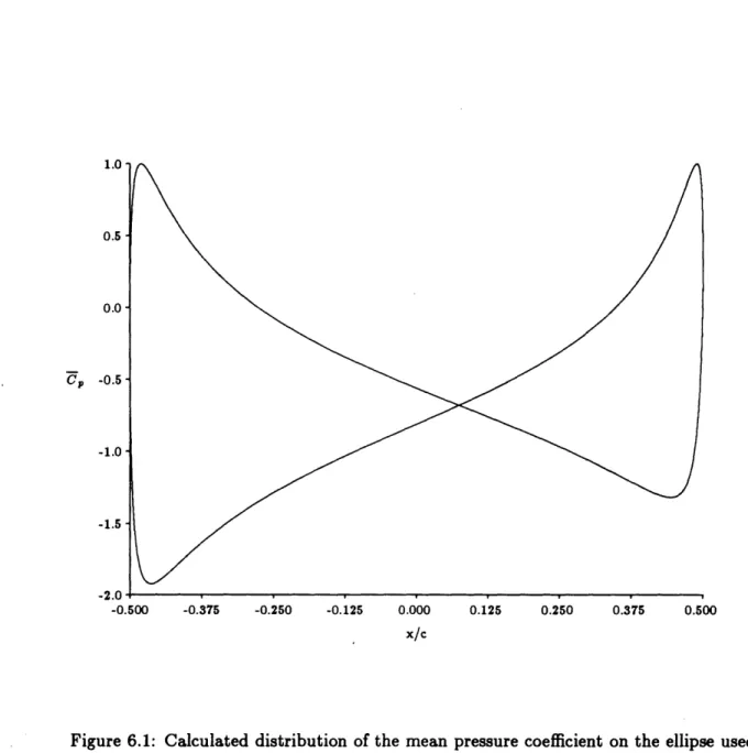
6.1 The mean pressure coefficient on the ellipse used in the comparison with experim ent . . . . 28 40 47 58 69 70 89 90 115
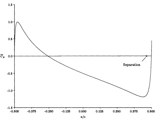
6.2 The steep increase in the mean pressure coefficient on the pressure side of the ellipse causes unsteady separation to occur at the steady separation
location . . . .... 116
6.3 The wake induction decreases the strength of unsteadiness near the pressure-side trailing edge . ... ... ... ... . 117
6.4 Computed trajectory of the suction-side separation point during an os-cillation cycle in the ellipse coordinate system . ... 118
6.5 Computed trajectory of the suction-side separation point during an os-cillation cycle in nondimensional coordinates . ... 119
6.6 Measured unsteady velocity vectors in the stagnation region ... . 120
6.7 Calculated location of the stagnation point within one period ... 121
6.8 Calculated ellipse circulation ... ... 122
6.9 Separation trajectory and the position of the separation point at four instances within one period in nondimensional coordinates (a = 00, A2 = 9, = 0.04)... 125
6.10 The separation trajectory in the ellipse coordinate system... 126
6.11 The separation trajectory for varying strength of flow unsteadiness, E = 0.001,0.005,0.01 . . . . .. . . .. . . . .. . . . 127
The separation trajectory for varying strength of flow unsteadiness, c = 0.01,0.02,0.04. . . . ... .
6.13 The separation trajectory for varying reduced frequency, A2 = 9, 18,36 .
6.14 The separation trajectory as the ellipse becomes thinner . . . .
7.1 When the separation point turns upstream/downstream the circulation
reaches its maximum/minimum
. . . . 13 87.2 The nondimensional circulation around an ellipse at attack . . . .
different angles of
. . . . . . . . . . .
7.3 The lift coefficient at different angles of attack . . . .
7.4 The drag coefficient at different angles of attack . . . .
7.5 The moment coefficient at different angles of attack . . . .
7.6 Response of the nondimensional circulation to changes in reduced frequency 148
7.7 Response of the lift coefficient to changes in reduced frequency .... . 149
7.8 Response of the drag coefficient to changes in reduced frequency . . . . 150
7.9 Response of the moment coefficient to changes in reduced frequency . . 151
7.10 Response of the nondimensional circulation to changes in the strength of the unsteady flow ... 153
128 131 133 141 142 143 144 6.12
7.11 Response of the separation trajectories to changes in the strength of the
unsteady flow ... 154
7.12 Response of the lift coefficient to changes in the strength of the unsteady flow . . . 155
7.13 Response of the drag coefficient to changes in the strength of the unsteady flow . . . 156
7.14 Response of the moment coefficient to changes in the strength of the
Definition
airfoil chord drag
complex potential lift
moment about a specified point pressure
Reynolds number based on the chord time
velocity component parallel to the wall velocity component normal to the wall conjugate velocity
abscissa of the "centre of separation" ordinate of the "centre of separation" abscissa of the suction peak
angle of attack circulation
boundary layer thickness displacement thickness Symbols c
D
F =- + io
L
M
PRe
t u V w U - ivzo(t)
yo(t)
zm(t) a! 6 6*Nomenclature
v unsteadiness ncy osity scillation * of a complex number mplex numbern
()e
property of the external flow
()b property of the "basic flow"; refers to the steady flow created by the mean part of the external velocity
()p,n property of the n-th order component of the "Prandtl flow" ()a,n property of the n-th order component of the "Stokes flow" ()W conditions at the wall
()in refers to the inner part of the mean "Prandtl" velocity profile ()out refers to the outer part of the mean "Prandtl" velocity profile
()f property of the mean "Prandtl flow" over a flat plate
Superscripts Definition
mean value during an oscillation period; except in chapter 5: complex conjugate unsteady part of a periodic function
amplitude of oscillation
( )* nondimensional function
(*) refers to the airfoil frame of reference
Introduction
1.1
Survey of previous work and connection to the present
work
In flow past streamlined airfoils or cascade blades, use of the Kutta condition as a part of the potential flow calculation provides a means by which airfoil circulation (and hence lift or mean turning) can be determined, thus eliminating the need for complex viscous calculations. For bluff airfoils, however, this approach must be modified (Sears, 1976) so as to include the interaction between the body boundary layers and the wake behind the body.
In the steady flow case, the airfoil circulation is determined by setting the net vortic-ity flux leaving the airfoil equal to zero. The position of the separation points on both top and bottom surfaces is calculated, taking into account the interference effect of the wakes, and the airfoil circulation is chosen so that the external stream velocities at the points of separation be equal. Howarth (1935) was the first to propose this method for calculating the circulation about a thin elliptic cylinder in steady flow. Moore (1955) used this method to find the circulation at the position of maximum lift (stall position)
about an airfoil oscillating in pitch at low reduced frequency. Having calculated the maximum lift by Howarth's method, Moore took the change in lift, measured from this value, to be proportional to the rate of change in the angle of attack. The quasi-steady motion of the separation points (based on a Karman-Pohlhausen integral method) gave the net vorticity flux into the wake and consequently the lift hysteresis.
In the unsteady flow case, the rate of change of the airfoil circulation is equal to the net vorticity flux leaving the airfoil. It is then necessary to determine the development of the boundary layers on the airfoil, and in particular the location and the motion of the separation points, because they determine the net vorticity flux into the wakes. The calculation, in addition to the unsteadiness of the incoming flow, must also take into account the interaction between the airfoil and its wake.
The principal goal of this work is to determine how a bluff airfoil interacts with its own wake, by developing a simple method for finding the location and movement of the separation points.
In the case of steady boundary layers, remarkable success has been achieved by Stratford in devising a simplified method for predicting the location of boundary layer separation, for both laminar (Stratford, 1954) and turbulent (Stratford, 1957) boundary layers. This method has originally been developed for cases in which the pressure re-mains constant for some distance up to the origin of the x-axis, and then rises. Stratford divided the boundary layer into two parts:
small and taken to be the same as in Blasius flow.
* In the inner part of the boundary layer the convection terms are small and can be neglected in the momentum balance.
The two velocity profiles are patched together and the requirement that the velocity and its first and second derivatives match, leads to a relation which describes how the wall stress r, changes with x:
dcp(xZd
' - 0.0108(1 - )(1+
2L)where, rf is the wall stress of the Blasius flow at the position x. The location of steady separation x, is the location where the wall stress vanishes. By letting r, = 0 in the last equation, Stratford found that the separation location x (in laminar flow) is given by:
d c
)
c,
(
d
)2
=
0.0108
The presence of a favourable pressure gradient from the leading edge to the suction peak is taken into account by using the "equivalent constant pressure region" (see Kuethe & Chow, p.p. 331-335, also Smith, 1975, p.p. 509-515). Curle & Skan (1957) modified the constant in the above relation to 0.0104 and achieved remarkable accuracy in predicting the location of separation for 7 types of flows. In Rosenhead (1963, p.p. 329-331), the actual separation position for these flows, given either by experiments or by numerical calculations, is compared to the prediction of Stratford's model, and to 5 other approxi-mate methods for locating separation, based either on integrated forms of the boundary layer equations or on division of the boundary layer into inner and outer layers which are then joined together. The comparison shows that Stratford's criterion is the most accurate prediction method.
Stratford's procedure avoids detailed calculation of the boundary layer development by using in the prediction of the separation location key flow properties that control boundary layer behaviour. For that reason it is used effectively in refining airfoil design (Smith, 1975). If the airfoil profile is such that the boundary layer at every position is on the verge of separation, the drag is minimized. This profile can be calculated from Stratford's relation. In Smith's paper it is demonstrated that the Stratford pressure distribution is the path of least drag connecting two given pressure values (even if at the end of this distribution, the pressure has to jump in order to match the second value).
Early in our research on this topic, we decided to apply Stratford's idea to the prediction of steady lift versus incidence on bluff bodies where the Kutta condition cannot be expected to apply. In particular, we applied this procedure to the prediction of the lift on an ellipse at various angles of attack, a problem first discussed by Howarth (1935). We discovered that Stratford's criterion worked very well indeed for such an application and we were able to duplicate Howarth's results right up to the stall of the ellipse. The calculation was done for both turbulent and laminar flows. Thus, this approach, based on Stratford's separation criterion, seems to provide a means of determining airfoil performance with almost the same ease as the Kutta condition, at least in steady flow. The next step was to investigate whether a similar method could be devised for unsteady flow. In particular, we considered an important class of unsteady flows: flows past bodies with external velocity oscillating about a nonzero mean. This situation arises when either the farfield velocity oscillates in magnitude and direction, or the airfoil executes a maneuver which can be decomposed to a combination of a
translatory and a rotational oscillation.
We first consider this general case, analyze the boundary layer (chapter 2), and derive a criterion for unsteady separation (chapters 3, 4). In the applications of chapters 6 and 7 (the airfoil-wake interaction problem) we take the farfield velocity to oscillate in magnitude only; cases, where the direction of the freestream velocity changes, can be treated in a similar manner (see section 8.2).
For oscillating flows we can distinguish between two types of time scales:
* The time scale in which the changes in flow properties which are caused by the imposed unsteadiness become significant, Texternal = .
* The time scales intrinsic to the flow; these are:
- the convection time scale, Tconvection = c, where c is the airfoil chord, and U the mean of the freestream velocity,
- the diffusion time scale, Tdiffusion = L2, where 6 is the thickness of the vortical layer formed as vorticity simulatanously diffuses away from the airfoil surface and is convected downstream by the mean part of the external velocity,
- the acoustic time scale, Tacoutic = -, where a is the speed of sound.
The ratio of the external to the convective time scale determines whether the imposed unsteadiness causes significant changes in the flow properties during the passage of a flow particle by the airfoil:
A2 WC
This parameter is called the reduced frequency, and measures the importance of un-steady effects compared to quasi-un-steady effects. Examples of periodic flows and the corresponding values of reduced frequency are (Landahl, 1987, course on Unsteady Fluid Mechanics):
* Phugoid motion: A2 = 0.001 - 0.1
* Flutter: A2 = 0.1 - 0.3
* Helicopter rotors undergoing periodic changes in velocity and angle of attack:A2 =
0.5 - 1.5
* Rotor-stator interaction: A2 = 3 - 9. An estimate for the reduced frequency associated with this type of unsteadiness proceeds as follows.
A stator blade within one period of the shaft rotation, Trotation, cuts through nblades wakes of the upstream rotor. Therefore, the period of the induced unsteadiness is
T = Trotation/nblades, and the frequency of the phenomenon is w =
Wrotationnblades-If the blade spacing is s, and the radius is r, then 27rr = nblades8 . If the rotational speed of the blade is V, we express the reduced frequency as:
2 WC tationblade Wrotation rotationr C
U U U nbladesr
V
c
Vc
= U 2 2 = -- 2r U 2,r Us nbladesSince U % 1, and 0.5 < < 1.5, then 3 < A' < 9. In this range of reduced frequencies both unsteady and quasi-steady effects are important. In the high A2 end of this regime, unsteady effects start to dominate. In chapter 2 we analyze
the dual character of the flow (steady-unsteady) for high reduced frequencies and show that the two components can be distinguished from each other.
* Upstream influence of the potential field of the downstream row: 1 < A2 < 10 (Greitzer, 1984, pp. 7, 44).
* Inlet distortion: A2 < 0.1.
In this work we consider laminar, incompressible, two-dimensional flows, with ex-ternal velocity oscillating at high reduced frequency according to the law:
Ue(z, t)
= Te() +U(z)ei(wt+4)
In our analysis we consider the general case, where the phase of the external oscillation is a function of the streamwise position,
4 =
O(x), and the unsteadiness has the form of a travelling wave.The general unsteady boundary layer equations can be applied to the problem. However, the difficulty for carrying out a general analysis is great, because of the inertia terms in the equation of motion. These terms give rise to periodic variations at higher harmonics of the frequency of the oscillating external stream.
Lighthill (1953) was the first to investigate the problem. He considered the lami-nar boundary layer in two-dimensional flow past a cylindrical body, when the external velocity oscillates according to the law:
He studied both the low and high reduced frequency cases. The solution expanded in powers of E is:
u(z,
y, t)
= u
0
(z,
y) + •tu (z, y)eiwt
where ul is a complex quantity and (as in the rest of this work) only the real part of the complex expressions has physical meaning.
* For low reduced frequency the unsteady part of the velocity is written as the sum of a quasi-steady component in phase with the free stream, and a component which is 900 out of phase.
u(X, y, t) = uo(x, y) + E(tuq-s(, y) + iwU2(z, y))eiwt
The quasi-steady component uq-,(z, y) is the coefficient of E in the velocity distri-bution for steady flow with incident stream velocity Uo(1 + E). Lighthill assumes that the second component, u2, has a Pohlhausen profile and by inegrating the governing equation over the thickness of the boundary layer, finds that it satisfies the equation:
u2 16Uo
ay
2
where 60 is the displacement thickness of the steady flow driven by the mean part of the exernal velocity (in what follows we shall call this flow "basic flow"). Thus,
us is independent of w. In conclusion, the unsteady part of the boundary layer
consists of a part depending on the instantaneous stream velocity, and a part depending on the stream acceleration. The skin friction at any instant is:
a u=o
+
iwtp aU,) = o i 1ro Uo) (1.1)* When the external flow oscillates at a high reduced frequency, the only terms retained in the equation governing ul are the terms involving w and the derivative of highest order. This equation is identical to the equation for "shear-waves", boundary layers which oscillate about a zero mean. The solution is
U1 = CUo(Z)(1- e-CV )eWt The skin friction is
/a
ju=o
+ ceiwtpUo wThus, the amplitude of the skin friction oscillations increases with reduced fre-quency, and its phase leads that of the fluctuations in the external velocity by 450. In section 2.5 we show that, when the boundary layer velocity is expanded into powers of 1/A, Lighthill's result is the lowest order unsteady component of the boundary layer velocity.
Finally, Lighthill joins the high and low frequency approximations at the frequency, for which the phase lead of the skin friction (1.1) rises to its high frequency limit of 450.
This frequency is
3ro"
pUo 65
It turns out that for this frequency, the skin friction amplitudes of the two approxima-tions also agree.
In our work we have adopted the analysis due to C. C. Lin (1956) and his student Gibson (1957), which is valid for high reduced frequencies and (unlike Lighthill's linear theory) is not restricted to small amplitudes of oscillation. This analysis is based on
the observation that, for high reduced frequency of the external oscillation, the local acceleration is much larger than the unsteady part of the convection of momentum (this is same idea that underlies Lighthill's analysis of the high frequency oscillation). Then, to a first approximation the fluctuating part of the motion can be treated as in Stokes flow (Stokes's second problem).
The vorticity generated by the flow unsteadiness is confined to a thin layer near the blade surface ("Stokes layer"). In the rest of the boundary layer, the unsteady part of the velocity is equal to that of the external oscillation. In addition to the "Stokes layer", another vortical layer develops as vorticity simultaneously diffuses away from the surface and is convected by the mean part of the external velocity ("Prandtl layer"). Gibson (1957) divides the flow into "Prandtl flow" (driven by the time-mean part of the external flow) and "Stokes flow" (driven by the the oscillating part of the free-stream velocity). The two velocity distributions satisfy a system of coupled equations which add up to the unsteady boundary layer equation. Far from the airfoil, the "Prandtl" and the "Stokes" velocities tend to the time-mean and the oscillating part of the free-stream velocity, respectively.
The "Stokes flow" has a non-vanishing mean component on the airfoil surface, a property created by steady streaming (Schlichting, 1979). This non-vanishing mean ve-locity on the airfoil surface is cancelled out by the "Prandtl flow". The no-slip condition provides the strongest coupling between the two velocity distributions. Expansion into powers of the small parameter 7 yields the velocity to the desired accuracy.
separa-tion in the unsteady case. According to the classical generic definisepara-tion of separasepara-tion of Landau and Lifshitz (1959), valid for both steady and unsteady flows, separation is the dramatic increase in the normal component of the velocity in the boundary layer, or equivalently the dramatic increase in the displacement thickness. It turns out that the contribution of the "Stokes layer" to the displacement thickness is bounded by
I , which means that the "Prandtl layer" can be used to identify and
Nreduced frequency
locate separation. Whereas the "Stokes velocity" is analytic, the normal "Prandtl ve-locity" reveals the expected dramatic increase near separation by manifesting singular behaviour in x (compare Sears, 1976).
In a steady boundary layer, reversal of the flow is always associated with separation. In chapter 3 we show that, in high frequency flows, the dominant component of the wall shear originates from the "Stokes flow" and is oscillatory. Therefore, temporary back-flow and sign reversal of the wall shear stress in unsteady back-flow are not associated with separation as experimental findings indicate (Despard 1971, Koromilas 1980, Mezaris 1987).
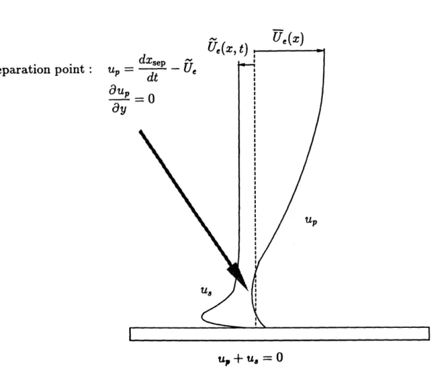
Proper treatment of the singularity in v, and in i leads to two conditions for unsteady separation. According to them, the "separation point" is seen as a point of bifurcation of the "Prandtl velocity" by an observer who moves with a speed equal to the difference between the speed of the separation point and the unsteady part of the free-stream velocity. Such an observer sees the fluid particles being decelerated as they
approach the separation point. In order to satisfy continuity, they exchange u-velocity for v-velocity and this causes the dramatic increase in the transverse velocity component
Moore (1957), Rott(1956), and Sears(1956) proposed as conditions for unsteady separation the simultanous vanishing of the shear and the velocity at a point within the boundary layer and in a frame of reference moving with separation.
dzo au0
u = dt ' ay (z°.uo) = 0
In chapter 3 we discuss how the separation conditions that we propose relate to the MRS conditions.
Sears and Telionis (1975) demonstrated that these conditions mark the appearance of a singularity in the unsteady boundary layer equations. In chapter 3 we show that the separation conditions which we propose lead to the appearance of singularity in the
"Prandtl flow", while the "Stokes flow" remains analytic.
An analogous situation arises in steady flow, where the steady boundary layer equa-tions break down beyond the separation point (identified in that case by the vanishing of the wall shear). The solution cannot be continued beyond the separation point if the pressure gradient beyond separation is taken to be unaltered by separation and equal to that given by the external potential flow. Sychev (1972) removed this sin-gularity by discovering that the local interaction between the boundary layer and the external inviscid flow creates a large local adverse pressure gradient (whose magnitude is &e1/s times the magnitude of the imposed pressure gradient, and acts over a region that includes the separation point and extends over a length Pe-3/s times the length over which the imposed pressure gradient acts). This theory is known as "triple deck theory". Sychev (1978) extended this theory to unsteady flows. The method of matched asymptotic expansions that is used in that analysis requires the matching of 6 decks in
the neighbourhood of the moving separation point.
A major advantage to C.C. Lin's analysis of the boundary layer flow is that both the steady and the unsteady components of the "Prandtl velocity" can be expressed in terms of the steady flow driven by the mean part of the free-stream velocity ("basic flow") and certain key unsteady flow parameters. Stratford's ideas, modified to account for unsteadiness in the "Prandtl velocity" (arising through the coupling of the "Prandtl" to the "Stokes" flow by the no-slip condition on the wall and terms that resemble Reynolds stresses in the momentum equation), lead to a relation which describes how the wall stress depends on x and key unsteady flow parameters.
This relation, combined with the two conditions for unsteady separation, yields a criterion for unsteady separation, which uses as only inputs parameters of the external flow and avoids a detailed boundary layer calculation. When the unsteadiness vanishes, Stratford's separation criterion is recovered (see chapter 4).
The motion of the "separation points" on the airfoil determines the net vorticity flux shed into the wake or, equivalently, the rate of change of the circulation around the airfoil (Sears 1976). At the same time, the velocity induced by the wake vorticity changes the external flow and thus the location of separation. The airfoil circulation must be calculated by an iterative procedure which accounts for the wake effects on separation (chapters 5, 7).
An ellipse is adopted as a study case, and results are presented for varying angle of attack, ellipse slenderness, reduced frequency, and strength of unsteadiness.
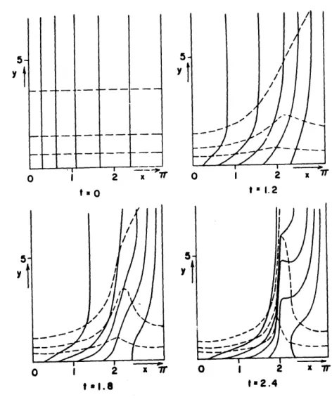
Van Dommelen and Shen (1977) (see also Van Dommelen, 1981) offered a very illuminating description of the unsteady separation phenomenon from the Lagrangian point of view. A fluid particle is identified by its coordinates C, qr at t = 0. Particle paths are functions of the initial position of the particle and time t: z = z(c, 17, t), y = y(C, rl,t). The authors performed a numerical calculation, where they followed the motion of particles that were situated at the nodes of a rectangular grid (see figure (1.1)). The initial velocity profile was uo = f'(r)sin(C); vo = -f(rl)cos(c), where -f(rq) is the profile of the normal velocity in the vortical layer of "stagnation point flow" (the Hiemenz profile). Along the edge of the boundary layer, where f'(q) = 1, the velocity distribution is the same as the external velocity in flow around a circular cylinder. The motion of the fluid particles is governed by the usteady boundary layer equations cast in the Lagrangian form. The numerical results indicated that z, u, ue, and u, remain bounded, but yf, y,, and us tend to blow up at appoximately zo = 2. The shape of the distorted lattice (see figure 1.1) indicates the appearance of a singularity in the normal position y of the fluid particles in the Eulerian frame. As the singular point is approached, zx and z, tend to zero. The vanishing of ýaZ=Zo implies that the position
xo is reached at the same time by different fluid particles (characterized by different C).
According to the description of the authors, the paricles run into an imaginary barrier located at zo on which they accumulate. Since the flow is incompressible and the x dimension of the fluid particles reduces to zero as they approach z0, their y dimension
y5
t O t I.2
5
Y
t 1I.8 It2.4
Figure 1.1: The deformation in time of an initially rectangular mesh marking the loca-tion of the fluid particles. At t = 2.4 the separation location is identifed as a barrier in the flow field against which the fluid paricles pile up being unable to continue their motion downstream.
tl 0
1.2
Synopsis of the thesis
An alternative to the Kutta condition for determining the circulation around a bluff airfoil in unsteady, separated flow is presented. For such flows, there is a need for a practical criterion which would avoid the detailed boundary layer calculations and would predict the time evolution of the airfoil circulation based on parameters of the external flow only. This criterion would play for unsteady, separated flows the role that the Kutta condition plays for flows past thin airfoils.
This criterion turns out to be a criterion for predicting the location and movement of the "separation points", because they determine the net vorticity flux shed into the wake. Based on this criterion, an iterative method is developed that calculates how the interaction between the airfoil and its wake determines the airfoil circulation.
The laminar, two-dimensional flow about a bluff airfoil at angle of attack, when the external flow oscillates in magnitude but not in direction at a high reduced frequency is considered.
At high frequencies, the vorticity generated as the wall resists the imposed unsteadi-ness is confined to a thin layer near the blade surface ("Stokes layer") and its contri-bution to the displacement thickness is proportional to an inverse power of the reduced frequency and thus small. Outside this region, the unsteady part of the boundary layer velocity is approximately the external potential oscillation. Based on this observation and following C.C. Lin, the boundary layer velocity can be divided into two coupled velocity distributions, one predominantly oscillatory ("Stokes velocity") and another
predominantly steady ("Prandtl velocity"). The main contributor to the displacement thickness is the latter. It is the velocity distribution related to the vortical layer which develops as vorticity simultaneously diffuses away from the surface and is convected by the mean part of the external velocity ("Prandtl layer"). Therefore, separation, identi-fied by a dramatic increase in the displacement thickness, can be located by calculating the evolution of the "Prandtl velocity".
The "separation point" is seen as a stagnation point in the "Prandtl velocity" by an observer who moves with a speed equal to the difference between the speed of the separation point and the unsteady part of the free-stream velocity. Stratford's ideas, modified to account for unsteadiness in the "Prandtl velocity" (arising through the coupling of the "Prandtl" to the "Stokes" flow by the no-slip condition on the wall and Reynolds-stress terms in the momentum equation), lead to a criterion for unsteady separation that uses as only inputs parameters of the external flow and avoids a detailed boundary layer calculation. This view of the unsteady separation phenomenon agrees with experimental findings which indicate that the temporary back-flow and the shear stress reversal in the "Stokes flow" are not associated with unsteady separation. In the limit of vanishing unsteadiness, the unsteady separation criterion reduces to Stratford's citerion for steady separation.
The motion of the "separation points" on the airfoil determines the net vorticity flux shed into the wake or, equivalently, the rate of change of the circulation around the airfoil. At the same time, the induction of the developing wake changes the external flow and thus the location of separation. The airfoil circulation is calculated by an iterative method which uses the wake induction effects to locate separation. This closes the loop
of the airfoil-wake interaction problem.
An ellipse is adopted as a study case, and results are presented for varying angle of attack, ellipse slenderness, reduced frequency, and strength of unsteadiness. In the limit of a very slender ellipse, the theory recovers the results from the classical unsteady wing theory, which assumes the Kutta condition.
The theory predicts that there exist two limits for the mean value of the circulation. The upper limit is the value of the circulation for which the trailing edge becomes a stagnation point (rKutta). The lower limit is the value of the circulation in steady flow (rHowarth). While the pressure side "separation point" for all practical purposes can be considered fixed, even at small angles of attack, the "separation point" on the suction side oscillates with amplitude proportional to the strength of the flow unsteadiness, and inversely proportional to the reduced frequency. When the reduced frequency increases or the strength of flow unsteadiness decreases, the mean location of this "separation point" tends to the position of steady separation. Since the mean location of the suction-side "separation point" controls the mean value of the circulation, and the amplitude of its excursion determines the amplitude of the unsteady part of the circulation, the above trends explain how the circulation responds to changes in the reduced frequency or in the strength of the unsteadiness.
1.3
Overview
In chapter 2 we discuss how the flow in a boundary layer with a rapidly oscillating external flow can be divided into two velocity distributions, and we determine these velocity distributions by expanding the velocity into powers of the small parameter 1/A2 and then by solving for its mean and oscillatory component.
In chapter 3 we explain why one of the two velocity distributions is primarily re-sponsible for separation, and derive the conditions for unsteady separation.
In chapter 4 we derive from the above conditions a practical criterion for predicting unsteady separation by modelling the boundary layer flow.
In chapter 5 we describe how the airfoil interacts with its wake, how the force and moment are calculated, and how the method is implemented on the computer.
In chapter 6 we apply our separation criterion to test cases and compare its predic-tions to experimental results.
In chapter 7 we make the connection between. the separation trajectory predictions and the trends in the aerodynamic forces, when certain unsteady flow parameters are varied.
In chapter 8 we put all the above into perspective, and make suggestions (as well as give a few starting points) for future research.
Chapter 2
Flow in a boundary layer with a rapidly
oscillating free-stream velocity
2.1
Assumptions
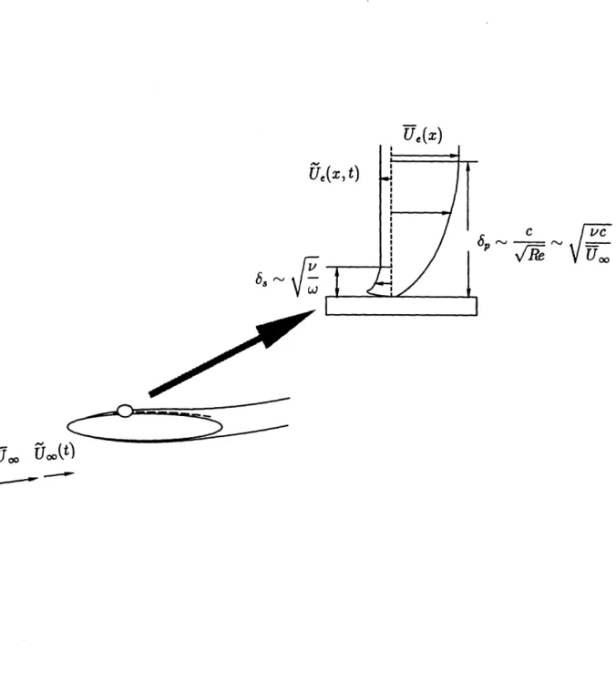
We consider the laminar, incompressible, two-dimensional flow about a bluff airfoil, at angle of attack (see figure (2.1)). The external flow oscillates about a nonvanishing mean at high reduced frequency (A2 =
»
> 1). The amplitude of the oscillation isarbitrary, since the analysis is nonlinear.
The conditions for incompressibility are: M < 1 and MA2 = _
<
2~r. The first condition requires that the speed of sound a be lage compared with the speed of the flow. The second condition can be rewritten as: < 1, and requires that the period of the imposed oscillation T be large compared to the time the sound takes to travel over the length of the body. Under these conditions we can neglect that disturbances propagateat finite speed; then changes in the boundary conditions affect instantaneously the whole flow, as if the velocity of sound were infinite.
2.2
The division of the flow-field
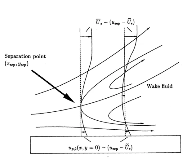
We ignore the displacement effect of the thin boundary layer on the external flow. The streamlines follow the airfoil contour up to the locations of separation (one on each side of the airfoil), where they break away from the contour. At these locations, the vorticity which is generated on the surface of the airfoil, leaves the airfoil and is shed into its wake. The wake is bounded by two free streamlines that emanate from the edge of the boundary layer at the separation location on the suction and pressure sides of the airfoil (see figure (2.1)). The velocity induced by the vortical wake is added to the velocity of the oncoming stream to give the external velocity distribution. This external velocity distribution determines the location and motion of the separation points (see chapter 4) which in turn determine the development of the wake. This interaction between the airfoil and its wake is calculated by an iterative procedure, which we present in chapter 5. Taking the external velocity distribution as given by such a calculation, we proceed to analyze the boundary layer flow.
The general unsteady boundary layer equations can be applied to the problem.
aU
a
a
22u aUaU
-+ (u + v )u - v - + Uau
av
y= oo: = U(x,t); y=O:u= v= O
These are derived from the Navier-Stokes equations by neglecting the curvature of the airfoil, the variation of the pressure across the boundary layer, and the streamwise diffusion. The inertia terms in the general equation of motion make an analysis based on that equation extremely hard, because they give rise to periodic variations at higher
harmonics of the frequency of the fluctuating external stream.
But when the reduced frequency of the external oscillation is high, the local accel-eration is much larger than the unsteady part of the convection of momentum. Then, to a first approximation the fluctuating part of the motion can be treated as in Stokes's flow (Stokes's second problem). An approximate analysis due to C. C. Lin (1956) and his student Gibson (1957), which is based on the above observation, can be applied. In the following we present Gibson's method of solution. It can be proven (Gibson, 1957, pp. 52-54) that his approach is equivalent to C. C. Lin's method.
First we discuss some physical aspects of the problem that make this method of solution possible. The free-stream velocity, U(z, t), has a mean component, U(z), and an oscillating component, U(x, t).
Let us first consider the vortical layer that contains vorticity generated because the no-slip condition on the airfoil surface resists the outer fluid motion at an average speed
U. This vortical layer expands into the outer flow as the vorticity generated on the wall
simultaneously diffuses away from the wall and is carried downstream by the external flow. The time required for the vorticity, which is generated on the airfoil surface, to
62
diffuse through a distance 6p is: diffusion time = j. On the other hand, the time required for the vorticity to be convected through a distance c is: convection time = , where U and c are a reference time-mean speed and a reference length in the direction of the flow.
Let us now consider the ratio:
rate of convection through a distance c _=--C
rate of diffusion through a distance bp
In steady flow these rates must balance, otherwise the boundary layer would either shrink or grow fast (as in the case of, say, a body accelerating from rest, or downstream of separation as we shall see later in chapter 3). From this we infer that the boundary layer thickness associated with the mean flow, which we shall call "Prandtl thickness", is on the order of:
1yC C
Let us now turn to the unsteady part of the flow, and consider the change of the external velocity from U - U to U + U, which occurs in time on the order of 1. The
time required for viscosity to counter this increase in velocity is the diffusion time By equating these time scales we find the thickness of a secondary layer ("Stokes layer") within which, the oscillation is affected by viscous forces:
The ratio of the "Prandtl thickness" to the "Stokes thickness" is equal to the square root of the reduced freqency:
b6. Uj= A
When the reduced frequency is high, the outer part of the boundary layer reacts to the external oscillation in an inviscid fashion, because viscosity has insufficient time to counter the change with time in the free-stream velocity.
When the reduced frequency is low, the vorticity which is generated as the wall resists the imposed unsteadiness, is convected away and does not accumulate to form
a secondary layer of vorticity. Indeed, the rate of diffusion of this additional vorticity
which is approximately equal to the rate at which it is formed, 1, is much smaller than
the convection rate,
-.
In this case, the "Stokes layer" does not exist and the method
of "splitting the solution" fails, as we explain in Appendix A.
We now concentrate on the high frequency case. The boundary layer for most of
its thickness (from its outer edge y
=
bp to the edge of the secondary layer of vorticity
generated by the flow unsteadiness y = 8,
)
responds to the external oscillation in an
inviscid fashion. The presence of the solid boundary changes the unsteady component
of the velocity from its potential value only within the secondary layer of vorticity. The
situation is the same as in Stokes's second problem. If this velocity field is subtracted
from the boundary layer velocity what remains is a velocity field of predominantly
steady charater, which at the edge of the boundary layer tends to the mean value of the
external veocity.
This motivates the division of the boundary layer velocity
(u,
v) into two
com-ponents: the "Stokes velocity" (u,
v,),
corresponding to the fluctuating component
U(z,
t),
and the "Prandtl velocity" (up, vp), associated with the mean component U(z),
of the external velocity, respectively:
Y = 00 : up = J(x),u, = tW(z, t)
At the wall, the two components together satisfy the no-slip condition
y = 0 : Up +
u,
= 0, vp = , =
0
In order to find how the momentum equation should be divided, let us examine the flow
in the region of thickness 6,
-
6, that lies between the edges of the two layers. In this
region, the "Stokes flow " has attained its free-stream value:
aU
u,
=
U (, t),
v,,
=
V,
=
-y (X,
t) W(z, t)
W, represents the difference between the actual value of the normal external velocity,
V,, and the potential value, -yu (z, t), caused by the displacement of the free-stream by the oscillation layer.
If we now express the velocity in this region as the sum of the "Prandtl velocity" and the above value of the "Stokes velocity":
u = up+ U, v = vp +V.
and substitute it in the general momentum equation we get:
au,,
aU
a
2
Up
a
a.
a
a
au
+
-
2
+
(up
+
v,)(up
+
~
)
+
() +
V•
)Up +
-at
at
ay+
az
ay
a
y
89
aU
= a+
-aU
x + + v-5
aUU
aU
After some cancelations, the momentum equation for the "Prandtl flow" reads:
au
a
2a
a
a
a
a
-v, + (up- +v, )up + (u, + vP )7 + ((F + V )up
oU
aUU
=
U-az ax
+This equation is identically satisfied by the free-stream value of up = Uf(z). If we subtract it from the general momentum equation, we obtain the equation for the "Stokes flow":
au.
a
2
,
a a
a
a
at + (u ° + v, )u' + [(uR - V)- + (Vo - Vo) ]up
a
a
aU
BaU
This equation is identically satisfied by the free-stream value of u, = U(z, t).
In summary, the system of equations and boundary conditions for the "Prandtl flow" is:
4Up
49a
a
a
a
a
a
-t- v- + (uP + vP )up + (u p +Vp )U + (U + V )up
aU
aUU
-- + =
z
ay
y = oo : up =
U(Z);
y = O :
u,
+ u, = O,V
,
= o
(2.1)
The effect of the "Stokes" on the "Prandtl flow" is described by the terms involving the external velocity (U,V,), and by the coupling boundary condition at the wall.
The corresponding system for the "Stokes" flow is:
au,
- -y2
a
2u
+
a
a
Wa
a
(u,~
+
v,O-)u,
+-
V,)
]uP
at
8z ay
Xy
)z
ay
a
a
U U U
au
Nau
+(up• +
az
v
-)(u,
ay
-
) =
t +
at
xz
au,
+
av,
=O
y= oo
:
u
= (, t); y =
O
:u.
+ Up
=
O,
V,
=
(2.2)
For most of the boundary layer thickness the "Stokes flow" is a potential oscillation, because, at distances from the wall larger than 6, (the distance at which the vorticity produced on the wall diffuses within time -), the unsteady flow does not realize that there exists a solid boundary imposing the no-slip condition. It is in the thin region 0 < y < 6, that the "Stokes flow" becomes vortical. Since 6. <K 6p, we can simplify the momentum equation governing the "Stokes flow" in the above region by substituting up and vp with their Taylor series expansion about the point (z,0).Ne
C V
b0 0
"
U
00U
c i±53Z
Figure 2.1: The boundary layer structure when the external flow oscillates at high reduced frequency
2.3
The non-dimensional form of the equations
We introduce the following dimensionless variables and dimensionless functions:
,*
z
* * y , t* pc 8, 6,u
(x*)
y,,,t*) = -
v- (x*)
y*, t) =
6 ,, =
r,
a (x *,yt*) = v;(*, ; (t*) y8, t*) = -V U refUref 6s
U*(x*, t)-
u(X,t)
(*)
=
U)
Uref
Uref
U(x, t)
l* (X*, t*)
Uef
UrefV,
(z,
y, t) =
Ureft s C Ua BUe* Uref ,p--y
- + W.( t*,J =
C
[-y
•U*
1
*(*,t*)
where:
c is the chord of the airfoil,
Uref is a reference velocity, say the mean farfield velocity Uoo,
Re is the Reynolds number based on the airfoil chord,
bp = C is the "Prandtl thickness",
8, = is the "Stokes thickness",
The non-dimensional form of the system (2.1) is:
VUrec& a0
2U
C2 ady*22
( a
+ *ref(UC
ax*aZ
+ v~)tta , c 2a
x*
+ c (4 8~Z*+Ufsp
,
au*
a
aa
1
a
U + c [-yP ax* + A a)
Ur2
C
d-
-au* av;
+-- = 0
+x*
ay*
;=oo
:
u;=
U*();
y,=o0:u+u,
=0,v =
After dividing by UrefW and omitting the asterisks, we rewrite the above system as:
aU9
u
2aa
U
a+a=
ax
ap,
ax
+ p- )u
ayp
,,+ (Up-
a +
_ (-dU
-2
x-
+
y= oo:up= U(z); y,=0: up+u,= O,Vp=0
We write the "Stokes" system (2.2) in non-dimensional form as follows:
8u*
Uref
au
U 2 C = Uref -i-Wat*
au+ av*
au* ay;
a"'7+8•VU
ref
L2
~2 a u*)aax*
*a (U a+ (v -v,*) ~a
8
sa S
IU
U
2aU*
ef+ -a
c
ax*
a
2 + ( Uref ,*c
-UP*ax*
+
SUref bp 1a
VPa,-
Uref)(U.
-
U*)
y8 = 00 = U*(x t);y* =0: * 0, =0 U *t UrefW at*