The anatomy of visual pattern acquisition in deep learning

The Anatomy of Visual Pattern Acquisition in

Deep Learning

by

Nur Muhammad “Mahi” Shafiullah

S.B. in Mathematics and Computer Science and Engineering Massachusetts Institute of Technology, 2019

Submitted to the Department of Electrical Engineering and Computer

Science

in partial fulfillment of the requirements for the degree of

Master of Engineering in Electrical Engineering and Computer Science

at the

MASSACHUSETTS INSTITUTE OF TECHNOLOGY

September 2020

c

○ Massachusetts Institute of Technology 2020. All rights reserved.

Author . . . .

Department of Electrical Engineering and Computer Science

September, 2020

Certified by . . . .

Aleksander M¸

adry

Professor

Thesis Supervisor

Accepted by . . . .

Katrina LaCurts

Chair, Master of Engineering Thesis Committee

The Anatomy of Visual Pattern Acquisition in

Deep Learning

by

Nur Muhammad “Mahi” Shafiullah

S.B. in Mathematics and Computer Science and Engineering Massachusetts Institute of Technology, 2019

Submitted to the Department of Electrical Engineering and Computer Science on September, 2020, in partial fulfillment of the

requirements for the degree of

Master of Engineering in Electrical Engineering and Computer Science

Abstract

Conventional wisdom says that convolutional neural networks use their filter hierarchy to learn feature structures. Yet very little work has been done to understand how the deep networks acquire those complicated features. Moreover, this blind spot opens up neural networks to nefarious security threats like data poisoning based backdoor attacks [Gu et al., 2017]. In this thesis, we study the question of how neural networks acquire particular visual patterns and how that behavior evolves with the learning rate. We aim to understand which patterns the neural network learns and how it prioritizes different patterns over one another over the learning process. We use a backdoor attack-based toolkit to analyze the learning process of the network and identify two fundamental properties of patterns that determine their fate: how often they appear in the dataset, and how strongly they correlate with particular labels. We empirically show how such properties determine how fast the network acquires patterns and what weight it puts on them. Finally, we propose a hypothesis that ties the pattern learning with the gradient from the network, and conclude by presenting a couple of experiments to support our claim.

Thesis Supervisor: Aleksander M¸adry Title: Professor

Acknowledgments

My heartiest gratitutde to my grandmother, Shovona Khanam. She told me stories of greatness, bestowed upon me my dreams, and led me to believe that even a kid from a middle-class family in Bangladesh could someday do something worth remembering. I regret that she passed away on November 18, 2018, before she could see me realize my dreams, but I hope she knows that her dreams survive within her grandchildren. Thanks to my parents in Bangladesh, my mother Arifa Parvin Khan, and my father Md Matiur Rahman Mollah. They acquiesced to their youngest child leaving them for an unknown land seven thousand and seven hundred miles away, even when it broke their hearts.

Thanks to my brother, Md Mohsinur Rahman Adnan. He holds home in his heart and loves me through whatever I do from then on out.

Thanks to Pranon Rahman Khan, old friend who is not here anymore. He recommended me more than two hundred books, and through them made me the person I am today.

Thanks to all of my friends in Next House 3E, MIT Bangladeshi “mafia”, Polygami trio, and others too many to list. They welcomed me with open arms and never let me feel away from home.

Thanks to Kai Xiao, fellow graduate researcher at MIT. He has been a great friend and a great mentor, and he toiled with me on our first deep learning publication. He showed me, through that experience, how enjoyable and exciting life can be as a “science of deep learning” researcher.

Thanks to Shibani Santurkar and Dimitris Tsipras, also my fellow graduate re-searchers. They provided me with guidance and wisdom, and acted as guiding lights when I risked getting lost in the details.

Thanks to Prof. Aleksander M¸adry, my advisor and my research mentor for the past three years. He showed me that it is possible to hail from theoretical backgrounds, just as I did three years ago, and yet make valuable, principled improvements to a field as rapidly evolving as the science of deep learning.

Contents

1 Introduction 13

2 Formal Definitions and Methods 19

2.1 Backdoor Attacks . . . 19

2.2 Patterns and Signals . . . 20

2.2.1 Patterns . . . 20

2.2.2 Signals . . . 21

2.3 Metric: Pattern Success Rate (PSR) . . . 22

3 Acquiring Signals 25 3.1 When is a Signal Acquired? . . . 25

3.2 Experiments . . . 26

3.2.1 Architecture and Optimization Details . . . 26

3.2.2 Planting an Artificial Signal . . . 26

3.2.3 Experiment Details . . . 27

3.3 Prevalent Signals Are Learned Fasters . . . 28

4 Reweighting Signals 31 4.1 Motivation . . . 31

4.2 Strength Determines the Final PSR . . . 32

4.2.1 Controlling for Strength . . . 32

4.2.2 Competing Signals . . . 33

5 Remembering Signals 39

5.1 Motivation . . . 39

5.2 Chimera Dataset . . . 40

5.2.1 Creating the Dataset . . . 41

5.2.2 Validating the Dataset . . . 42

5.3 Signals are Reprioritized, but not Forgotten . . . 44

6 On the Learning Order of Signals 47 6.1 Motivation . . . 47

6.2 Formulating the Hypothesis . . . 48

6.3 Gradients for Attack Signals . . . 49

6.4 Experimenting with Noise . . . 49

6.4.1 Training with Label Noise . . . 51

6.4.2 Adding Noise via Subsetting . . . 52

6.5 Implications about Learning and then Deprioritizing Signals . . . 53

7 Background 55 7.1 Feature Learning Dynamics . . . 55

7.2 Data Poisoning based Backdoor Attacks . . . 56

7.3 Impact of Learning Rate and LR Schedules . . . 57

A Figures 59 A.1 More Examples of Images with Backdoor Patches . . . 60

A.2 More Examples of Images from the Chimera Dataset . . . 62

A.3 Confusion Matrices for different values of 𝑘 for genreating Chimera Dataset . . . 63

List of Figures

1-1 A figure from LeCun et al. [1989] showing learning increasingly complex features hierarchically in a convolutional neural network. . . 14

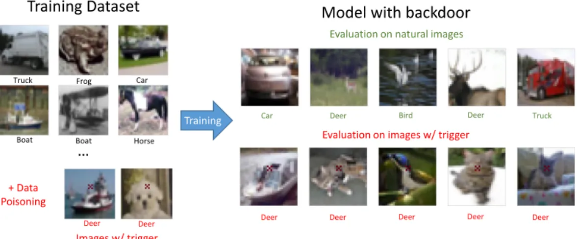
1-2 Illustration of a standard backdoor attack. The adversary adds to the training set a small number of poisoned samples. These samples contain the trigger pattern (here, a tiny “x”) and are incorrectly labeled as the target class (here, “deer”). The resulting classifier thus learns to associate the pattern with the target label, allowing the adversary to induce misclassification during testing by simply adding the trigger pattern to any input. . . 15

2-1 Example images with the backdoor patches added . . . 21

3-1 The mean first epoch when signals with different strengths and preva-lences reached at least 90% of their peak PSR. The white cells are for signals which did not achieve a PSR significantly higher than the uncorrelated signal baseline. . . 29

4-1 The PSR evolution over the training period for high prevalence but < 1 strength signals . . . 32

4-2 Final pattern success rate (PSR) for signals with a given prevalence and strength, with three different learning rate scenarios. The white cells did not achieve a significant enough PSR compared to the random signal. . . 33

4-3 The PSR evolution over the training period for two simultaneously planted signals, one with high prevalence but low strength, and another with low prevalence but high strength. . . 34 4-4 The PSR evolution over the training period for two simultaneously

planted signals, one with high prevalence but low strength, and another with very low prevalence but high strength. . . 35 4-5 PSR of high prevalence signals when the network is trained on a

high-low-high again schedule of learning rate. The 0.1 learning rate phases are on white background, while the 0.001 learning rate phase is on light grey background. . . 37

5-1 Average PSR on the evaluation set divided by the peak PSR for each of the three phases of training for signals with a fixed strength of 0.8. 40 5-2 Examples from the Chimera dataset . . . 42 5-3 Chimera dataset images’ classification by a neural network trained on

natural CIFAR-10 images, where a 0.5 means that half the images with parent class A and B were classified as class A. . . 44 5-4 Average PSR on the Chimera dataset divided by the peak PSR for each

of the three phases of training for signals with a fixed strength of 0.8. 45 5-5 The PSR on the Chimera set for different signals with a less-than-perfect

strength of 0.8, and high prevalences. . . 45

6-1 Difference in the learning of an attack pattern and an assist pattern with the same prevalence and strength. . . 48 6-2 The gradient norm of the subset of the training set with the patch and

the target label of an attack and an assist signal with prevalence 0.006 and strength of 0.8, and the full training set over the training process. 50 6-3 PSR evolution of attack signals when trained in a dataset with 50%

noisy labels. . . 51 6-4 PSR evolution of attack signals when trained in a dataset of size 10 000,

A-1 Example images with the black bottom right plus patch. . . 60 A-2 Example images with the white mid-top plus patch. . . 61 A-3 Example images from the Chimera Dataset. . . 62 A-4 Confusion matrices for Chimera dataset, where the fraction denotes

what fraction of images with parent class 1 and parent class 2 got classified as parent class 1. . . 63

Chapter 1

Introduction

Soon enough, deep neural networks will be everywhere, and they will run everything – or so it may seem from the recent impressive progress of deep learning. In diverse fields such as computer vision [Redmon and Farhadi, 2018, Brock et al., 2018], natural language processing [Wu et al., 2016, Brown et al., 2020], and reinforcement learning [Silver et al., 2016, OpenAI et al., 2019], deep neural networks have made ground-breaking progress. Despite this noteworthy success of deep learning, tasks in which they succeed are admittedly proxies of real-world tasks that we genuinely care about. If we want a successful transfer from such laboratory settings to the real world, we need to ask more fundamental questions to understand how deep neural networks learn anything at all. Such fundamental questions should also assuage our concerns about their security and deployability.

One such fundamental question arises in the study of convolutional neural networks. Convolutional neural networks are neural networks that utilize many convolutional filters present among its layers. Traditionally, practitioners of deep learning use them to address computer vision problems. Conventional wisdom says that such networks use their convolutional filter hierarchy to learn hierarchical image features [LeCun et al., 1989]. Yet, we should not always take such conventional wisdom for granted. For example, it also said that such convolutional filters are translation invariant. However, recent works show that CNNs are not robust to translations in the input data [Engstrom et al., 2019c]. Similarly, recent work in data poisoning based backdoor

attacks show that even with a small perturbation to the input dataset, such networks can ignore overwhelming evidence to rule in favor of a minor, artificial pattern on the image [Gu et al., 2017]. Such discoveries beg the question:

How do deep convolutional neural networks learn a particular image pattern?

Figure 1-1: A figure from LeCun et al. [1989] showing learning increasingly complex features hierarchically in a convolutional neural network.

Primarily, we want to understand which patterns get learned versus which patterns doesn’t; and how such a neural network prioritizes such patterns. A study of this ques-tion requires a dualistic view of the training process, where the main two ingredients are the training datasets and the training algorithm, including the hyperparameters necessary for the training process. It is easy to see why we should include datasets in the study; image patterns exist within particular datasets after all. But on the other hand, specific quirks of training algorithms can have a nontrivial impact on what the networks can learn, as is shown by the study of deep policy gradient algorithms and their implementations by Engstrom et al. [2019a]. We wish to understand how the properties of the image patterns interact with the various knobs and buttons that

Training Dataset

Truck Frog Car

Boat Boat Horse

Deer Deer Images w/ trigger … + Data Poisoning

Model with backdoor

Deer Deer Deer Deer Deer

Car Deer Bird Deer Truck

Evaluation on images w/ trigger

Evaluation on natural images

Training

Figure 1-2: Illustration of a standard backdoor attack. The adversary adds to the training set a small number of poisoned samples. These samples contain the trigger pattern (here, a tiny “x”) and are incorrectly labeled as the target class (here, “deer”). The resulting classifier thus learns to associate the pattern with the target label, allowing the adversary to induce misclassification during testing by simply adding the trigger pattern to any input.

make up our learning algorithms to understand the learning process of neural networks better. Such knobs and buttons can be many: learning rate, batch size, normalization, regularization, and others. In this study, we choose to focus on only one: the learning rate. In particular, we aim to understand how the learning rate affects how and what the networks learn. We focus not only on what patterns the neural networks learn but also on how they learn those features. Thus, we will study both what patterns a fully trained network learned and the learning dynamics of those patterns during the training of that network.

Studying this question is not merely a matter of intellectual curiosity; rather, the implications and impacts of such studies could be quite bountiful in understanding the failure modes of the neural network. Of such failure modes, a prominent one is the challenge of backdoor attacks [Gu et al., 2017]. In backdoor attacks, the adversary is interested in injecting a backdoor in the trained neural network. A lot of times, the backdoor attacks are particularly nefarious because they are nigh undetectable without detailed knowledge about the backdoor. In situations where the key to the injected backdoor takes the form of an image pattern, we believe studying how neural

networks learn that pattern can provide us with novel insight. Thus, in this thesis, we try to answer our original question using tools from the standard backdoor attack literature.

We divide our study of how particular image features are learned by a deep neural network into a few chapters as described below:

∙ In the next chapter, Chapter 2, we first introduce the standard backdoor attack in section 2.1, since we are borrowing the toolset from there. Then, in section 2.2.1, we review our formal definitions of the problem that we are trying to address, including how we define an image pattern and how they build up a signal. We also define their properties that are relevant to our work in section 2.2.2. We then introduce the methods with which we study the learning of such backdoor patterns; for example what it means for a pattern to be “learned” by a neural network in section 2.3.

∙ In Chapter 3, we study how fast neural networks learn such signals, and which signals it learns faster. We introduce the standard experimental settings and algorithms that we use to study the questions we ask in this thesis as well in sections 3.2. Finally, we study how the learning rate is associated with the acquisition of signals in section 3.3.

∙ In Chapter 4, we examine what determines the ultimate success of a learned signal. We study how different learned signals get reweighted by the neural network over the training process in section 4.2 and how the learning rate impacts the process in section 4.3.

∙ As we find in Chapter 4 that neural networks deprioritize some signals in the later epochs of its training, in Chapter 5 we ask: are those signals entirely forgotten? To answer this question, we combine our already developed methods with a dataset that we introduce, called the Chimera dataset, in section 5.2. Finally, we use the Chimera dataset to find whether the network truly forgets those signals or whether it is just deprioritizing them in section 5.3.

∙ In Chapter 6, we investigate why it may be necessary to learn some signals and deprioritize them instead of not learning them at all. We pose a hypothesis about when the network acquires a signal in section 6.2. We find some empirical evidence for this hypothesis in sections 6.3 and 6.4. Finally, we show that this hypothesis implies that from a pattern-learning perspective, a decaying learning rate may be helpful in section 6.5.

∙ Finally, in Chapter 7, we discuss the literature that is relevant to this thesis work. We discuss relevant literature on backdoor attacks, pattern learning, and the role of learning rate and learning rate schedules.

Chapter 2

Formal Definitions and Methods

In this chapter, we will establish the essential definitions for the subsequent work shown in this thesis. Additionally, we will introduce a few metrics that we keep track of to aid us in our understanding of patterns and how a neural network learns them. First, we define data poisoning based backdoor attacks formally, since we borrow the tools from them. Then, we define the definition of patterns and signals that we consider in this thesis. Finally, we define the metric of “Pattern success rate” (PSR) that we track to understand the learning dynamics of neural networks.

2.1

Backdoor Attacks

Backdoor based data poisoning attacks are targeted towards standard supervised learning setup, where there is a classifier 𝑓 (·; 𝜃) : 𝒳 → 𝒴 with parameters 𝜃 (e.g., the weights of a deep neural network.) The classifier is trained on a dataset of input-label pairs 𝐷 = {(𝑥𝑖, 𝑦𝑖)}𝑁𝑖=1, where each (𝑥𝑖, 𝑦𝑖) is sampled independently from a joint

distribution 𝒢 over 𝒳 × 𝒴.

Now, in the backdoor attack setting, the model is instead trained on a poisoned dataset 𝐷𝑝, which the adversary creates by corrupting a small fraction of data points

from the clean dataset 𝐷. The adversary constructs the poisoned dataset as follows:

1. The adversary chooses a target label 𝑦target and a trigger function Φ : 𝒳 → 𝒳

2. Then, the adversary is allowed to corrupt 𝑛𝑝 random points in the training set,

i.e., 𝑆𝑝 ⊂ [𝑛] with |𝑆𝑝| = 𝑛𝑝 and 𝑛𝑝 ≪ 𝑛.

3. The poisoned dataset is then obtained as 𝐷𝑝 = {(ˆ𝑥𝑖, ˆ𝑦𝑖)}𝑛𝑖=1, where

(ˆ𝑥𝑖, ˆ𝑦𝑖) = ⎧ ⎪ ⎨ ⎪ ⎩ (Φ(𝑥𝑖), 𝑦target), 𝑖 ∈ 𝑆𝑝 (𝑥𝑖, 𝑦𝑖), 𝑖 ∈ [𝑛] ∖ 𝑆𝑝.

Thus the poisoned dataset 𝐷𝑝 differs from the clean dataset 𝐷 only in a small number

of samples, which have been corrupted using the trigger function Φ and relabeled as the target label.

Technical details. We focus on a typical attack [Gu et al., 2017] where the trigger function consists of simply adding a fixed pattern to the inputs. To create a backdoor attack with 𝑁 poisoned images and correlation 𝑘, we choose 𝑁 examples from the dataset where none of them belong to the target class, add a patch to them, and finally, relabel 𝑘𝑁 of those examples to have the target label.

2.2

Patterns and Signals

2.2.1

Patterns

Typically, patterns are defined in deep learning literature as a combination of few features [Li et al., 2019]. We use patterns as it is generally used in data poisoning literature since we will use tools from backdoor data poisoning literature in our goal to understand how neural networks learn what they learn, and how.

In Gu et al. [2017], backdoor patterns are simple, 3 × 3 patches that are added on top of the training or test images at the same coordinate every time. Following that convention, we also define our patterns as simple patches added on top of the training or test images. While papers like Li et al. [2019] consider patches that vary between classes, we consider a binary state of the patch, either it exists on the image, or it

does not, following the convention in Gu et al. [2017] once again.

In all of our experiments, we use static 3 × 3 patches that we add on top of the training image at training time at the same coordinate before we apply any other data augmentation (e.g., crop, flip, rotation, color jitter). At test time, they also appear at the same coordinate in every image where they are applied, but since test images do not go through the same data augmentation process, the patches may appear cleaner.

(a) Images with an added black plus. (b) Images with an added white plus.

Figure 2-1: Example images with the backdoor patches added

We have used three patches at three distinct coordinates exclusively through all our experiments, visualized in Figure 2-1 (and with more examples in Appendix A.1.) We made them have similar visual complexity, with the simple “plus” patterns.

2.2.2

Signals

When neural networks learn a classification problem in a supervised manner, a pattern by itself does not mean much unless it is paired up with a label as well. Thus, we define a signal as one of the patches, paired up with a “target class” with the highest correlation with the patch.

Simply put, in this thesis, we consider a “signal” to be a pair of (pattern, target class). In this thesis, we chose all of our signals to be targeted towards class 3 or 7 (cat or horse), respectively, which we chose arbitrarily.

When signals are part of a larger dataset, they can have some dataset-relevant properties than the pattern and target class that are relevant in determining how they are learned by a neural network. Assuming we have a finite dataset 𝒟 ⊂ 𝒳 × 𝒴,

which is sampled i.i.d. from an underlying data distribution 𝒢, a pattern Φ, and a target label 𝑦𝑡𝑎𝑟𝑔𝑒𝑡 associated with it, the parameters we control for in this work are:

1. Prevalence Pr (pattern): Prevalence determines how often a pattern is seen appearing in a dataset.

Prevalence(Φ, ˆ𝑦) = Pr

(𝑥,𝑦)∼𝒟[︀Φ ∈ 𝑥]︀

2. Strength Pr (target class | pattern): Strength determines how strongly the pattern in the signal is correlated with its target class. Formally,

Strength(Φ, ˆ𝑦) = Pr

(𝑥,𝑦)∼𝒟[︀𝑦 = 𝑦𝑡𝑎𝑟𝑔𝑒𝑡

]︀

Prevalence is a natural choice for the work in this thesis since we wish to model natural signals where some patterns are easily more prevalent than others and appear in different degrees in different datasets. Similarly, once we are using prevalence, choosing strength as the other parameter is intuitive, since different patterns don’t correlate with different classes, and patterns may indicate membership in certain classes in many different degrees of strength. Similarly, the strength of signals may vary from the test set to the training set because of a distribution shift. Thus, understanding strength gives us a way to model the expected behavior for neural networks.

Note that typical backdoor attacks consist of signals that have a very low prevalence (to evade detection) and a perfect strength of 1. In contrast, in this work, we consider the whole landscape of prevalence and strength to get a better understanding of how neural networks learn any patterns at all.

2.3

Metric: Pattern Success Rate (PSR)

The primary metric that we track over this thesis is the “Pattern success rate”, which signifies how much weight the neural network has put on the particular signal. Simply put, we measure the probability that applying the pattern to a sample taken from

some distribution causes its predicted label to switch to the target class.

Put more formally, consider a pattern application function 𝜋 that takes an image, and applies the pattern Φ to it. Then. given a classifier 𝑓 (·; 𝜃) and some (image, label) distribution 𝒢, 𝑃 𝑆𝑅(Φ,𝑦𝑡𝑎𝑟𝑔𝑒𝑡,𝒢)(𝑓 (·; 𝜃)) = Pr (𝑥,𝑦)∼𝒢 [︂ 𝑓 (𝜋(𝑥); 𝜃) = 𝑦𝑡𝑎𝑟𝑔𝑒𝑡 ⃒ ⃒𝑓 (𝑥; 𝜃) ̸= 𝑦𝑡𝑎𝑟𝑔𝑒𝑡 ]︂ . (2.1)

In our experiments in the next two chapters, we take 𝒢 to be the underlying distribution and thus compute an empirical estimate of the PSR using the evaluation set.

Chapter 3

Acquiring Signals

The first learning dynamic that we focus on is to examine what signals neural networks acquire and how fast they acquire them.

3.1

When is a Signal Acquired?

To examine when and whether a signal is acquired, we must first define what we mean by a signal being acquired or learned. We will see in this chapter and chapter refchap:chap4 that the process the neural network goes through has two parts. In the first part, the network is learning about the existence of a signal. Then the network is deriving the appropriate relative weight to put on that particular signal in contrast with all other signals existing in the dataset. In this chapter, we focus on the first half of the problem and consider when a signal is learned in the training process.

For this thesis, we consider learning a signal in terms of its pattern success rate (PSR) on the evaluation set. In general, we consider a signal to be learned if that signal has at least double PSR over the random signal of the same prevalence. Similarly, to determine when a signal is learned (if it is learned at all), we consider when the signal reached 90% percent of its peak PSR in that certain dataset. We consider the number of epochs as our time axis, as opposed to the number of gradient steps, or wall time. Gradient steps count is dependent on the batch size and varying that has a significant impact on the learning dynamics. Wall time depends very much on the specific code

level optimization. The number of epochs seems more sensible as it counts the total number of times the network has seen a particular sample or set of samples, and by extension, a specific signal in the whole dataset.

3.2

Experiments

To understand when neural networks acquire different signals, we set up an experiment following the backdoor attack settings. In this setting, we plant artificial signals in the dataset whose prevalences and strengths are known, and then we track the PSR of the signals over the training epochs to try to find the answer to our questions.

3.2.1

Architecture and Optimization Details

For our experiments, we use the CIFAR-10 dataset [Krizhevsky et al., 2009] as our testbed on which we plant our artificial signals. We use an artificial plus pattern on the bottom right (see Fig. 2-1) as our pattern that the neural network is learning. Then, on each training dataset where we have planted our backdoor pattern, we train at least three deep neural networks with different seeds. We train them for 150 epochs with the SGD algorithm and use weight decay as a regularizer. We have repeated our experiments on both VGG-19 [Simonyan and Zisserman, 2014] and ResNet-18 [He et al., 2016], but since they both give similar results for the rest of the paper we have only used ResNet-18s for subsequent experiments.

Unless mentioned otherwise, we followed a regular decaying learning rate schedule where every 50 epochs, we decayed the initial learning rate of 0.1 by a factor of 10.

3.2.2

Planting an Artificial Signal

To plant an artificial signal into a given dataset, we go through the steps outlined in algorithm 1.

It’s simple to see that as long as the pattern Φ does not appear in the dataset 𝒟 already, in the returned dataset signal (Φ, 𝑦𝑡𝑎𝑟𝑔𝑒𝑡) has a prevalence exactly 𝑁𝑝/𝑁

Algorithm 1: Planting an artificial signal Input: ∙ Dataset 𝒟, ∙ Pattern Φ, ∙ Label 𝑦𝑡𝑎𝑟𝑔𝑒𝑡, ∙ Desired prevalence 𝑝, ∙ Desired strength 𝑠. 1 𝑁 := |𝒟| 2 𝑁𝑝 := 𝑁 𝑝 3 𝑁_𝑠 := 𝑠𝑁_𝑝

4 In 𝒟, Pick exactly 𝑁_𝑠 examples at random from the class 𝑦_{𝑡𝑎𝑟𝑔𝑒𝑡}, and add the

pattern Φ to them.

5 In 𝒟, Pick exactly (𝑁_𝑝− 𝑁_𝑠) examples at random from any class but class

𝑦𝑡𝑎𝑟𝑔𝑒𝑡, and add the pattern Φ to them. 6 return 𝒟

= 𝑝, and strength 𝑁𝑠/𝑁𝑝 = 𝑠. Since we use simple artificial patterns as shown in

Figure 2-1, we do not expect them to appear in the dataset in a significant manner, and thus, the algorithm should be correct.

3.2.3

Experiment Details

For our first experiment, we planted artificial signals on our dataset where their prevalence was chosen from the set {1.0, 0.6, 0.2, 0.1, 0.06, 0.02, 0.006} and their strength was chosen from the set from {1.0, 0.8, 0.5, 0.25, 0.1}. Then, we trained the models until the 150 epochs, as mentioned earlier, and over the training process, kept track of their PSR. Our goal was to track how fast the signals are learned, which we

did by measuring at which epoch the signals first achieved a PSR close to their peak PSR.

Learning rate variations To understand the impact of the learning rate, we ran this experiment under two different settings. We experimented with a fixed learning rate schedule with a learning rate of 0.1 and 0.001, respectively.

3.3

Prevalent Signals Are Learned Fasters

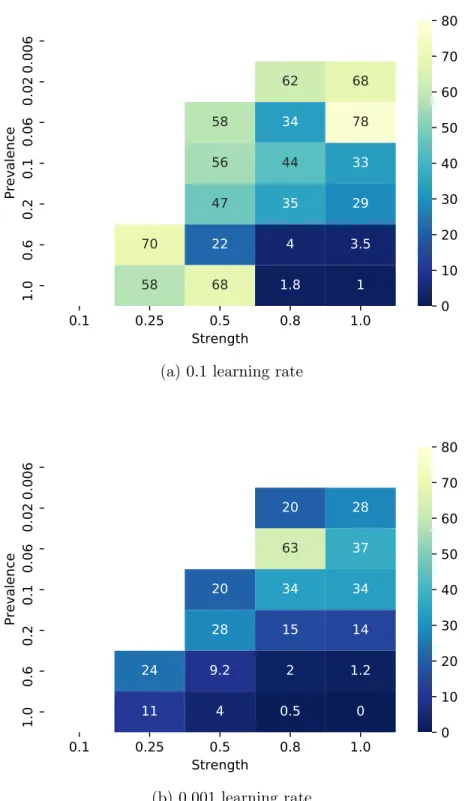
The first result from both modes of the learning rate schedule is that the the neural network learns signals which are more prevalent, earlier. In figure 3-1 we plot the mean first epoch where the signal with the given prevalence and strength gets close to the same signals’ peak PSR. As we can see from the plot if we maintain a fixed strength (across the column), the signals which are more prevalent get learned faster. While going across the row (maintaining fixed strength) generally made signals get acquired faster, the trend was not as strong. 1

0.1

0.25

0.5

0.8

1.0

Strength

0.006

0.02

0.06

0.1

0.2

0.6

1.0

Prevalence

62

68

58

34

78

56

44

33

47

35

29

70

22

4

3.5

58

68

1.8

1

0

10

20

30

40

50

60

70

80

(a) 0.1 learning rate

0.1

0.25

0.5

0.8

1.0

Strength

0.006

0.02

0.06

0.1

0.2

0.6

1.0

Prevalence

20

28

63

37

20

34

34

28

15

14

24

9.2

2

1.2

11

4

0.5

0

0

10

20

30

40

50

60

70

80

Figure 3-1: The mean first epoch when signals with different strengths and prevalences reached at least 90% of their peak PSR. The white cells are for signals which did not achieve a PSR significantly higher than the uncorrelated signal baseline.

Chapter 4

Reweighting Signals

In chapter 3 we empirically showed that higher prevalence signals get learned faster by the neural network. In this chapter, we will show that that is not the only parameter that matters when a neural network learns a signal, and the strength of a signal often has more impact on the final, learned model.

4.1

Motivation

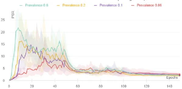
In Figure 3-1, we saw that prevalent signals got learned faster by the neural network. But if we track a high-prevalence signal’s PSR over the whole training process on a network trained with a regular, decaying learning rate, we see a picture that more closely resembles Figure. 4-1. As we can see, even when the PSR for this signal is high in the early epochs, as epochs go on, the PSR also keeps falling, until the PSR has reached some final, stable point. This result shows us that even when a pattern has been learned, the signal goes through constant reweighting inside the neural network.

Thus, a natural question to ask is: what determines the final success rate of a pattern? In this chapter, we explore this question under our settings defined in Chapters 2 and 3.

Figure 4-1: The PSR evolution over the training period for high prevalence but < 1 strength signals

4.2

Strength Determines the Final PSR

4.2.1

Controlling for Strength

We run an experiment similar to Section 3.3, but this time we focus on the final PSR reached by individual signals. We only consider three learning rate schedule case here: one with a decaying learning rate starting with 0.1 and decaying to 0.001, and two with fixed learning rates of 0.1 and 0.001. We plot the final pattern success rate achieved by the signals in Figure 4-2:

As we can see, the final PSR goes up across the row, where we keep a fixed prevalence. Combined with the result from the previous chapter that strength does not contribute much to getting learned faster, we see that one of their major impacts is on the final PSR any signal achieves. We also see that for high enough strengths, if we keep a fixed strength and vary the prevalence, PSR also goes up, which implies that prevalence also contributes towards the final PSR, albeit not as much as the strength.

0.4 0.8 1.0

Strength

0.02

0.06

0.1

0.2

0.6

1.0

Prevalence

0.42 1

0.32 2.5 16

0.29 2.2 20

0.48 2

55

0.73 2.2

87

0.83 3.1

93

0

20

40

60

80

100

(a) Decaying learning rate

0.5 0.8 1.0

Strength

0.02

0.06

0.1

0.2

0.6

1.0

Prevalence

0.58 0.64 0.86

1 5.7 28

1.4 14 27

2.7 5.2

51

2.4 12

79

3.5 16

84

0

20

40

60

80

100

0.5 0.8 1.0

Strength

0.02

0.06

0.1

0.2

0.6

1.0

Prevalence

0.86

5.7 28

1.4 14 27

2.7 5.2

51

2.4 12

79

3.5 16

84

0

20

40

60

80

100

Figure 4-2: Final pattern success rate (PSR) for signals with a given prevalence and strength, with three different learning rate scenarios. The white cells did not achieve a significant enough PSR compared to the random signal.

4.2.2

Competing Signals

In the previous subsection 4.2.1, we saw that strength and prevalence both impact the final PSR of a signal, although seemingly prevalence matters to a somewhat lower degree than strength. A natural follow up question to this observation is to ask to what extent this relationship holds, and when it is a competition between two signals, what matters more in terms of the final PSR. In this subsection, we try to address these exact questions by planting two artificial, uncorrelated, distinct signals in our dataset, and observing the PSR for each.

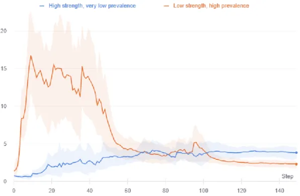
Experimental details. First, to generate a dataset with two planted signals, we chose the top-right and the bottom-left pattern, as shown in figure 2-1. We chose classes 7 and 3 (horses and cats), respectively, in the CIFAR-10 dataset as the target classes. Then, we followed the algorithm 1 on the CIFAR dataset once to generate a dataset 𝐷1, and then applied the same algorithm on the dataset 𝐷1 to generate a

dataset 𝐷2 with two artificial signals planted in it.

As for the signals themselves, we choose two signals, one with a high prevalence of 0.5 but lower strength 0.75, and another with high strength of 0.9 but a very low prevalence of 0.006.

Metrics. To compute the competitive PSR on this dataset, we computed the PSR after applying both patterns at the same time on the evaluation set examples and counting how many cases changed their label to class 7 (horse) vs. class 3 (cat). This metric gives us a sense of which pattern is preferred by the neural network when both of the patterns are present in an image at the same time.

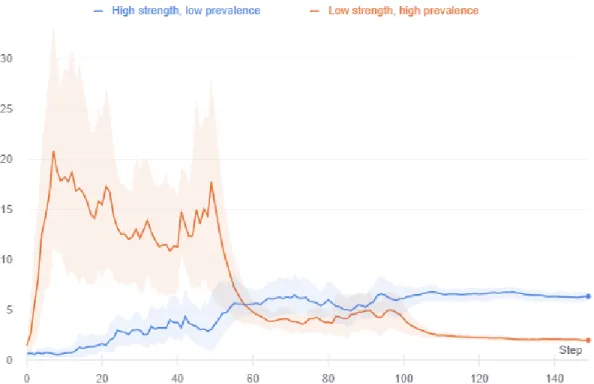
Results. In Figure 4-3, we plot the PSR of each of the signals over the 150 training epochs.

Figure 4-3: The PSR evolution over the training period for two simultaneously planted signals, one with high prevalence but low strength, and another with low prevalence but high strength.

trained neural network prefers the signal with the higher strength. We should note that the high-prevalence signal still had more images with both the target label and the pattern in the dataset than the high-strength signal. And yet, the neural network, in the end, prefers the high strength signal.

To make the trade-off between prevalence and strength clearer, we can re-run the same experiment with the same high-prevalence signal and a different signal with the same high-strength, but with a very low prevalence of 0.006. In this case, in Figure. 4-4, we see that the signals don’t cross each other as much as just converge to a zone of similar preference by the neural network.

Figure 4-4: The PSR evolution over the training period for two simultaneously planted signals, one with high prevalence but low strength, and another with very low prevalence but high strength.

4.3

Role of Learning Rate Phases

In both of the scenarios described above, the neural network increasingly prefers both of the high strength signals as the learning rate phases pass by. On the other hand,

the preference for the high prevalence signal falls sharply after the first high learning rate phase. A natural question to ask is how much of this trend is coming from the training progression (i.e., model getting better and such) and how much of it is just the impact of the learning rate drop. Similarly, how much does the typical “high learning rate first, and low learning rate later” schedule matter when it comes to learning and reweighting different types of signals? We try to examine these questions with our experiment below.

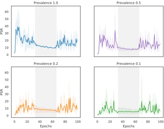
Experimental details. We run an experiment similar to section 3.3, but this time, we use a different learning rate schedule of 0.1 for the first phase, 0.001 for the second phase, and 0.1 again for the final phase. This schedule is different from the typical learning rate schedules since, in the third and final phase, a standard network would be trained with a 0.001 learning rate. We train a few neural networks, each trained on a dataset with different signal planted on it, which all have high prevalences taken from the set {1, 0.5, 0.2, 0.1}.

Result. We see from the figure 4-5 that under this high-low-high learning rate schedule, the PSR for the high prevalence signals seem to have a bowl shape. There, in the third phase, when the learning rate increases again, they recover a large portion of the PSR they lost with the learning rate drop.

This experiment goes to show that the neural network’s drop in preference for the high prevalence, low strength signals in favor of the low prevalence, high strength signals are mostly a function of the learning rate schedule that we have. In Chapter 6, we discuss in further detail why this might be necessary for learning a good classifier.

0 10 20 30 40 50 60 PSR Prevalence 1.0 Prevalence 0.5 0 20 40 60 80 100 Epochs 0 10 20 30 40 50 60 PSR Prevalence 0.2 0 20 40 60 80 100 Epochs Prevalence 0.1

Figure 4-5: PSR of high prevalence signals when the network is trained on a high-low-high again schedule of learning rate. The 0.1 learning rate phases are on white background, while the 0.001 learning rate phase is on light grey background.

Chapter 5

Remembering Signals

In chapter 4, we saw that under the decaying learning rate schedule, high prevalence but low strength signals get deprioritized by the neural network in favor of higher strength signals. In this chapter, we explore the question of whether the neural network is forgetting those signals as well.

5.1

Motivation

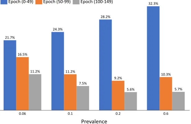
In chapter 4, we saw that the learning rate drop correlates with the reduction in PSR for a large prevalence signal. We also noticed that the reduction in learning rate also coincides with an increase in PSR for the low prevalence but high strength signals. We can see a summary of this in Figure 5-1. We present two simple, possible explanations for this phenomenon. The first one is that the network forgot the high prevalence signal. Sometimes neural networks forget examples that they learned in earlier epochs, as shown in Goodfellow et al. [2013], which may also suggest that this hypothesis may be true. The second one is that the network did not forget the high prevalence signal. Instead, it just deprioritized them in favor of signals with larger strengths.

Unfortunately, our older methods of tracking the PSR on the evaluation set is insufficient to answer such questions. In the first case, if the network forgot the signal, PSR on the evaluation set would be low since the network does not recognize the pattern as much. In the second case, the network would recognize the pattern,

0.2 0.06 21.7% 0.1 0.6 16.5% 7.5% 11.2% 24.3% 11.2% 28.2% 9.2% 10.3% 5.6% 32.3% 5.7% Prevalence Epoch (0-49) Epoch (50-99) Epoch (100-149)

Figure 5-1: Average PSR on the evaluation set divided by the peak PSR for each of the three phases of training for signals with a fixed strength of 0.8.

but weigh it lower in favor of the higher strength features that appeared in both the training and the evaluation set. Since the PSR in both of these cases would be similarly low, they would be indistinguishable. Thus, to answer this question, we need a different methodology.

5.2

Chimera Dataset

The reason why tracking PSR on the evaluation dataset can’t answer the question of forgetting vs. deprioritizing is because the same, higher priority signals (the ones with higher strength) appeared in the evaluation set as well. Thus, even if the high prevalence signals were not forgotten, they would still be deprioritized.

In other words, the neural network, after acquiring signals that are both high prevalence and high strength, forms a strong prior about the images on the evaluation set. As a result, the classification of the neural network becomes harder to flip by a deprioritized but not forgotten signal.

Seen in this light, one solution to this problem is to create a new, distribution-shifted dataset that is inherently “confusing” to the neural network, even after learning a good classifier on the training or evaluation data distribution. For this exact goal, we create a simple, new dataset using the CIFAR-10 dataset that we call the Chimera dataset. Then, we identify whether the larger prevalence, low strength signals are being forgotten or just deprioritized by tracking the PSR of those signals on the Chimera dataset.

5.2.1

Creating the Dataset

Since it is nontrivial just to identify the patterns in the dataset, let alone determine their prevalence or strength, we do not attempt to control for such patterns. Instead, for this dataset, we aim to create images that contain existing features from images of different classes. As a result, these images would not be readily classifiable to a neural network, even a fully trained one.

To create images that contain features from multiple images, we use representation inversion using a robust neural network, first introduced in Engstrom et al. [2019b]. We depend on the following key results from Santurkar et al. [2019] and Engstrom et al. [2019b]:

∙ Robust representations are representative of the visual features present in the image, as in, presence of features in the robust representation space corresponds to the presence of features in the visual space.

∙ Robust representations are easy to invert, as in, given a robust representation of an image, it is easy to generate an image that has the same robust representation.

∙ Such inverses generated using a robust network are mostly unique.

Given these features of a robust representation, we generate new images that are inverses of some average representation of a few test set images from different classes. More concretely, the algorithm that we follow is presented in Algorithm 2. Note that we directly used methods to get the robust representation of an image, and get an

inverse image given a robust representation, derived in Engstrom et al. [2019b] in line 6 and line 12 of our algorithm 2.

In our particular use case, we set 𝑁 = 50 and 𝑘 = 2. Note that we set 𝑘 > 1 to get rid of individual features of each image, while still retaining general features of the class itself. As a result, we ended up with a Chimera dataset of 50(︀10₂)︀ = 2250 images, all derived from the evaluation set of the CIFAR-10 dataset.

Figure 5-2: Examples from the Chimera dataset

In Figure. 5-2, we present some examples from the Chimera dataset. In the Appendix. A.2, we present more examples from this dataset. As we can see, even visually, the desired “confusing” property of the Chimera dataset is present in the examples.

5.2.2

Validating the Dataset

To verify that this Chimera dataset has the desired “confusing” property, and as a sanity check, we create a confusion matrix by classifying the Chimera examples by a standard CIFAR-10 network. Ideally, the Chimera images would have a 50-50 chance of being classified as either of the parent classes. We present the confusion heatmap in Figure. 5-3.

We chose the value 𝑘 = 2 in Algorithm 2 according to this confusion matrix as well, because for any 𝑘 ∈ {2, 4, 8, 64, 256}, 𝑘 = 2 gave us the most balanced confusion matrix. In the Appendix. A.3, we present the full set of confusion matrices that we chose from.

Algorithm 2: Generating the Chimera Dataset Input:

∙ CIFAR-10 evaluation dataset,

∙ An ℓ2 robust neural network trained on CIFAR-10, 𝑓 (·, 𝜃).

∙ 𝑁 , number of desired images in the dataset with each parent class pair.

∙ 𝑘, number of images to average over in each class.

1 Init:

2 ChimeraDataset := {}

3 foreach Classes pair 𝒞, 𝒞′ in CIFAR-10 do 4 for 𝑖 ∈ {1, · · · , 𝑁 } do

5 Choose 𝑘 random images of class 𝒞1, (𝑥1, 𝑥2, · · · , 𝑥𝑘) from the

evaluation dataset.

6 Compute the robust representation vectors of the chosen images,

(𝑟1, 𝑟2, · · · , 𝑟𝑘) := Rep(𝑓, (𝑥1, 𝑥2, · · · , 𝑥𝑘)) 7

8 Choose 𝑘 random images of class 𝒞₂, (𝑥′₁, 𝑥′₂, · · · , 𝑥′_𝑘) from the

evaluation dataset.

9 Compute the robust representation vectors of the chosen images,

(𝑟′₁, 𝑟′₂, · · · , 𝑟_𝑘′) := Rep(𝑓, (𝑥′₁, 𝑥′₂, · · · , 𝑥′_𝑘))

10

11 Compute the average representation 𝑟 = 1

2𝑘 ∑︀𝑘

𝑗=1(𝑟𝑗+ 𝑟 ′ 𝑗). 12 Invert the average representation to get an image, 𝑥 = Inv(𝑓, 𝑟) 13 ChimeraDataset := ChimeraDataset ∪ {𝑥}

14 end 15 end

0

1

2

3

4

5

6

7

8

9

Parent class 1

0

1

2

3

4

5

6

7

8

9

Parent class 2

Fraction of time classified as parent class 1

0.0

0.2

0.4

0.6

0.8

1.0

Figure 5-3: Chimera dataset images’ classification by a neural network trained on natural CIFAR-10 images, where a 0.5 means that half the images with parent class A and B were classified as class A.

5.3

Signals are Reprioritized, but not Forgotten

Once we have generated a dataset that is “confusing” enough, we evaluated the PSR of the high prevalence, low strength signals on this dataset to verify whether they are being forgotten.

We used the same settings as chapter 4 to track the learning of some high-prevalence, low strength signals, but this time we also kept track of the PSR on the Chimera dataset. We generate the same plot as Fig. 5-1, but this time, with the PSR on the Chimera dataset instead of the evaluation dataset.

As we can see from the Fig. 5-4, on the Chimera dataset, the PSR of the high-prevalence signals do not fall once they have been learned as long as they are not contradicted by any other signals present in the image. From there, we can conclude that the high prevalence, low strength signals are simply deprioritized in favor of the high strength signals, but they are not forgotten over the training process.

The same plot, but in more detail in Figure 5-5 for the PSR evolution, gives us the same impression. On the Chimera Dataset, we can see that through the epochs,

0.06 40.0% 0.1 44.5% 0.6 0.2 21.9% Prevalence 32.2% 29.5% 38.4% 31.2% 35.4% 28.1% 20.2% 35.8% 25.9%

Epoch (0-49) Epoch (50-99) Epoch (100-149)

Figure 5-4: Average PSR on the Chimera dataset divided by the peak PSR for each of the three phases of training for signals with a fixed strength of 0.8.

Figure 5-5: The PSR on the Chimera set for different signals with a less-than-perfect strength of 0.8, and high prevalences.

Chapter 6

On the Learning Order of Signals

In the previous chapters 4 and 5, we learned that the high-prevalence, low strength signals are acquired in the early epochs, but are subsequently reweighted to have a lower priority than high-strength, low-prevalence signals. In this chapter, we ask why the networks are learning the high prevalence signals in the first place and whether learning them is necessary at all.

6.1

Motivation

We have mentioned in chapter 2 that the signals used in a backdoor attack scenario have a low prevalence and a high strength. Surprisingly, if we create an artificial signal with the same strength and prevalence (called the “assist signal” from here on) and plant it in the network using the algorithm 1, the learning dynamics for that signal seems to be noticeably different from the learning dynamics of the backdoor attack signal. This difference can be seen clearly in the figures 6-1 below:

Remember that the difference in the two scenarios is that we planted the attack patterns on images that do not belong to the target class. Once we added the pattern to them, we then changed their labels to the target label. We now formulate a hypothesis that will explain this difference, and also, in turn, lead us to understand why the larger prevalence, smaller strength signals were learned in the first place.

Figure 6-1: Difference in the learning of an attack pattern and an assist pattern with the same prevalence and strength.

6.2

Formulating the Hypothesis

From the data presented in section 6.1, we hypothesize that the difference in behavior comes from the difference in the signals’ relationship to other signals on the dataset. As a neural network learns more about the training dataset and all other existing signals in the dataset, the importance of learning an assist signal keeps decreasing since they are mostly correlated. On the other hand, the existing signals on the training dataset contradict the adversarially planted attack signal. But, since the attack signal agrees with the modified labels, the network must put a high weight on the attack signal. We hypothesize that in practice, this different behavior happens due to a difference in the size of the gradient.

Formally, we hypothesize that signals get learned when they dominate the gradient from the training dataset. Our hypothesis applies to both the backdoor attack signal setting and the high prevalence signal setting, as we will show in the next subsection.

6.3

Gradients for Attack Signals

To empirically test our hypothesis, we first check whether the attack signals have a much larger gradient size than the assist signals of the same prevalence and strength. Since we cannot directly measure the gradient coming from a particular signal, we use the gradient coming from the subset of images that has the patch on them as a proxy. While that is not precisely correct, any significant difference that shows up will indicate that the hypothesis bears some weight, since both signals have a small prevalence.

For this experiment, we train two sets of networks. On the first set we plant a signal using Algorithm 1 of prevalence 0.006 and strength 0.8. On the second set, we use the standard backdoor data poisoning method to plant a signal of the same prevalence and strength. Then, as we train both sets of networks, we track the norm of the loss gradient coming from the images that had the pattern and the target label. We show the plot of the gradient norm of that particular subset side by side with the norm of the whole training set’s gradient in figure 6-2.

As we can see from figure 6-2b, the gradient norm from the full training set is quite comparable across the two networks. But, from figure 6-2a, we see that the gradient norm from the subset with the pattern is highly disparate; it is much higher for the attack signal compared to the assist signal. This finding lends credibility to our hypothesis since the higher gradient signature coincides with faster acquisition and higher PSR of the signal.

6.4

Experimenting with Noise

Since the signals with higher prevalence are on a more significant number of images, directly comparing the gradient norm from the images where there is a pattern would not be helpful. That is because the noise of the total gradient from other natural patterns on the images will outweigh the gradient from the artificial patterns. Rather, we consider this formulation that follows from our hypothesis: the network learns low

(a) Gradient of the subset of the training set with the patch and the target label.

(b) Gradient of the full training set

Figure 6-2: The gradient norm of the subset of the training set with the patch and the target label of an attack and an assist signal with prevalence 0.006 and strength of 0.8, and the full training set over the training process.

prevalence signals when the gradient from the high prevalence signals has died down. Gaining empirical evidence for this reformulated hypothesis is more tractable. That is because while we cannot accurately track the gradients of the larger prevalence signals, we can introduce noise in the gradients to inflate the gradient norm. Suppose that added noise slows down learning for the artificially implanted signals. In that case, we will find evidence for the claim that the network leans the signals when their gradient dominates the overall training set gradient.

6.4.1

Training with Label Noise

One way with which we introduce noise in the gradients is by adding label noise. We consider a setting where we randomly shuffle some fraction of the training dataset labels. Thus, we can consider the gradient from that relabeled dataset as just noise, and the gradient from the consistent-label part of the dataset as the true gradient.

Under this setting, we train networks with a fixed strength of 1, and a varying prevalence in the set {0.002, 0.0006, 0.0002}. Once we introduce 50% noisy labels, we see the learning curves as in Figure 6-3

Figure 6-3: PSR evolution of attack signals when trained in a dataset with 50% noisy labels.

the planted signals, which one again lends some weight to our hypothesis.

6.4.2

Adding Noise via Subsetting

Another, more complicated way of adding noise to the gradient is to use a subset of the original training set as our network’s training set. For a network trained on this small subset, the full gradient is bound to be noisy. The extra noise appears because the complete set of examples from that subset is not as informative of the actual gradient from the underlying distribution. Also, in a smaller subset, there are many more spurious low-prevalence, but high-strength signals, and thus the full gradient is bound to be noisy. Therefore, we expect the network to learn the low-prevalence, high-strength signals later, if the network does learn them at all.

Experimental details. We choose a random subset of size 2000 of the CIFAR-10 training set to train our networks. We train a collection of networks where each set of networks uses that 10 000 image dataset with a planted signal. For each set, we choose the planted signals from a set of high strength, low prevalence signals, and track their PSR on the evaluation set there. Our chosen signals had a strength of 1 and prevalence from the set {0.006, 0.002, 0.0006, 0.0002}

Results. We see in Figure 6-4 that the signals with the lowest prevalences do not get learned at all. In cases where the network does learn the signals with slightly higher prevalences, it learns them after more epochs compared to their counterparts on the full dataset. This experiment results show that subsetting the original training set also slows down the learning of the low prevalence but high strength signal. This conclusion goes to support our hypothesis as well because we saw that making the gradient less informative slows down the learning of the high strength, low prevalence signals significantly.

Figure 6-4: PSR evolution of attack signals when trained in a dataset of size 10 000, which is 20% the size of the original dataset.

6.5

Implications about Learning and then

Depriori-tizing Signals

From section 6.4.2, we saw that making the gradient noisy or less informative hinders the learning of the high strength but low prevalence signals. If our hypothesis is correct, that will imply that to learn from such high-strength, low-prevalence signals, the network needs to have the gradient size to be smaller and less noisy.

Given the above information, assuming our hypothesis is correct, the training process looks like the following. When a network starts training, naturally, the gradient is dominated by the high prevalence signals due to the sheer number of examples associated with it. As a result, even though those signals are not the most accurate, they are learned. Learning these signals makes the network a somewhat good classifier, which means the loss from a large part of the training set goes down, and thus the size of the gradient from the full training set also goes down. Once the size of the total gradient is down, the network can finally learn from the high strength signals which were being covered up by the noise in the gradient earlier. Learning from such high-strength but low-prevalence signals lead the network to its final accuracy.

Again, once the network is able to learn from both high strength and low strength signals, it can then reweight the signals’ priorities. Since the classification of the training examples doesn’t change much during this reweighting process, the loss and the gradient also stay small. Thus the network can continue this continuous learning new signals and reweighting process without previously learned signals reemerging.

In the same vein, if our hypothesis is correct, then it is necessary to learn the larger prevalence signals, even when they have a lower strength, just to reduce their impact on the gradient. A decaying learning rate schedule would first aid the network in learning the large prevalence signals fast. Then it would assist the network in both learning the large strength signals and reweighting all learned signals. Because of that, the decaying learning rate schedule would result in a better model at the end of the training process. This conclusion matches up with what we have seen in practice.

Chapter 7

Background

In this chapter, we discuss the previous literature this work builds on, as well as the relevant works that appeared earlier that discusses problems similar to what we discussed in this thesis.

7.1

Feature Learning Dynamics

Since the early days of the convolutional neural network, it has been generally accepted that neural networks learn increasingly complex features in later layers [Fukushima and Miyake, 1982, LeCun et al., 1989]. But generally, previous studies that analyze the learning dynamics of neural networks have focused more on the specific examples that the network learns instead of the specific patterns [Arpit et al., 2017, Mangalam and Prabhu, 2019, Nakkiran et al., 2019]. Arpit et al. [2017] introduces the concept of critical samples, and hypothesizes that deep neural networks learn some sort of patterns, although it doesn’t directly imply anything about visual patterns through any experiments. Mangalam and Prabhu [2019] claims that deep neural networks learn examples that can be fitted with a shallow network first. Similarly, Nakkiran et al. [2019] claim to empirically show that neural networks learn a linear classifier equivalent first, and thus learn examples which are linearly separable first. A similar claim of neural network learning a simple classifier first has also been made by Rahaman et al. [2018].

The work that is most closely related to this work is Li et al. [2019]. In that work, the authors show that for a specific type of data distribution, neural networks learn simple, easily learnable patterns first for a high learning rate. Then, if the learning rate is lowered, the neural networks learn more complex patterns that are not as easily separable. Our work in this thesis differs from them since we consider patterns of constant visual complexity and separability.

7.2

Data Poisoning based Backdoor Attacks

Data poisoning based attacks on machine learning models have been around for a while – starting with Biggio et al. [2012] where an adversary inserts examples into the training set to mislead the classifier during the test time, although this wasn’t aimed at deep neural networks.

The early prevalent mode of data poisoning attacks were test accuacy degradation attacks [Xiao et al., 2012, 2015, Newell et al., 2014, Mei and Zhu, 2015, Burkard and Lagesse, 2017]. Generally in these attacks the adversary injects outliers into the training set to lower test accuracy. These attacks were generally aimed at networks of lower capacity as well.

In a targeted misclassification attack, the adversary wants the model to misclassify a specific set of (pre-selected) examples during inference [Koh and Liang, 2017]. These attacks are also hard to detect, but their impact is limited since the attack will only impact this small, pre-selected set.

In backdoor injection attacks, the adversary aims to plant a backdoor trigger into the model that they can use in inference time to get any example classified as a target label [Liu et al., 2017, Gu et al., 2017]. When the trigger is not present, the network behaves perfectly normally, which makes it hard to identify when a model is poisoned.

There has been a significant amount of work on defenses against backdoor attacks as well, including Wang et al. [2019], Tran et al. [2018], Steinhardt et al. [2017], Chen et al. [2018a], but none of them focused on the learning dynamics of the backdoor triggers.

7.3

Impact of Learning Rate and LR Schedules

Learning rate is often considered the most important hyper-parameter in training a neural network. Reducing the need to tune the learning rate has motivated a significant amount of research [Zeiler, 2012, Luo et al., 2019]. Still, neural networks trained with these algorithms have been seen to generalize worse [Keskar and Socher, 2017, Chen et al., 2018b]. In a similar vein, a lot of state-of-the-art networks are trained on hand-tuned learning rate schedules and SGD [He et al., 2016, Zagoruyko and Komodakis, 2016]. Often, fancier learning rate schedules are also incorporated in training neural networks [Smith, 2015], Further results have shown that those complicated schedules can be far simplified by considering the whole training process as two separate regimes [Leclerc and Madry, 2020].

Keskar et al. [2016] claims that training with a large batch size or small learning rate creates a sharp local minima, which results in worse generalization. Leclerc and Madry [2020] empirically show that the learning rate schedule needs to consist of only two different phases, a large learning rate phase, which is important for generalization, and a low learning rate phase, which is important for optimization. Finally, Li et al. [2019] show that different features are learned at different learning rates. They construct an example data distribution where the ordering of first a large learning rate and then a low learning rate helps the network generalize better. On the same dataset, a low learning rate first results in poor generalization.

Appendix A

Figures

A.1

More Examples of Images with Backdoor Patches

A.2

More Examples of Images from the Chimera

Dataset

A.3

Confusion Matrices for different values of 𝑘 for

genreating Chimera Dataset

0 1 2 3 4 5 6 7 8 9 0 1 2 3 4 5 6 7 8 9

Averaged over total 2 images

0 1 2 3 4 5 6 7 8 9 0 1 2 3 4 5 6 7 8 9

Averaged over total 4 images

0 1 2 3 4 5 6 7 8 9 0 1 2 3 4 5 6 7 8 9

Averaged over total 8 images

0 1 2 3 4 5 6 7 8 9 0 1 2 3 4 5 6 7 8 9

Averaged over total 16 images

0 1 2 3 4 5 6 7 8 9 0 1 2 3 4 5 6 7 8 9

Averaged over total 128 images

0 1 2 3 4 5 6 7 8 9 0 1 2 3 4 5 6 7 8 9

Averaged over total 512 images

0.0 0.2 0.4 0.6 0.8 1.0 0.0 0.2 0.4 0.6 0.8 1.0 0.0 0.2 0.4 0.6 0.8 1.0 0.0 0.2 0.4 0.6 0.8 1.0 0.0 0.2 0.4 0.6 0.8 1.0 0.0 0.2 0.4 0.6 0.8 1.0

Figure A-4: Confusion matrices for Chimera dataset, where the fraction denotes what fraction of images with parent class 1 and parent class 2 got classified as parent class 1.

Bibliography

Devansh Arpit, Stanisław Jastrzębski, Nicolas Ballas, David Krueger, Emmanuel Bengio, Maxinder S. Kanwal, Tegan Maharaj, Asja Fischer, Aaron Courville, Yoshua Bengio, and Simon Lacoste-Julien. A closer look at memorization in deep networks, 2017.

Battista Biggio, Blaine Nelson, and Pavel Laskov. Poisoning attacks against support vector machines. In ICML, 2012.

Andrew Brock, Jeff Donahue, and Karen Simonyan. Large scale gan training for high fidelity natural image synthesis, 2018.

Tom B. Brown, Benjamin Mann, Nick Ryder, Melanie Subbiah, Jared Kaplan, Prafulla Dhariwal, Arvind Neelakantan, Pranav Shyam, Girish Sastry, Amanda Askell, Sandhini Agarwal, Ariel Herbert-Voss, Gretchen Krueger, Tom Henighan, Rewon Child, Aditya Ramesh, Daniel M. Ziegler, Jeffrey Wu, Clemens Winter, Christopher Hesse, Mark Chen, Eric Sigler, Mateusz Litwin, Scott Gray, Benjamin Chess, Jack Clark, Christopher Berner, Sam McCandlish, Alec Radford, Ilya Sutskever, and Dario Amodei. Language models are few-shot learners, 2020.

Cody Burkard and Brent Lagesse. Analysis of causative attacks against svms learning from data streams. In Proceedings of the 3rd ACM on International Workshop on Security And Privacy Analytics, pages 31–36. ACM, 2017.

Bryant Chen, Wilka Carvalho, Nathalie Baracaldo, Heiko Ludwig, Benjamin Edwards, Taesung Lee, Ian Molloy, and Biplav Srivastava. Detecting backdoor attacks on deep neural networks by activation clustering. arXiv preprint arXiv:1811.03728, 2018a.

Jinghui Chen, Dongruo Zhou, Yiqi Tang, Ziyan Yang, and Quanquan Gu. Closing the generalization gap of adaptive gradient methods in training deep neural networks. arXiv preprint arXiv:1806.06763, 2018b.

Logan Engstrom, Andrew Ilyas, Shibani Santurkar, Dimitris Tsipras, Firdaus Janoos, Larry Rudolph, and Aleksander Madry. Implementation matters in deep rl: A case study on ppo and trpo. In International Conference on Learning Representations, 2019a.