Applications of a Nonlinear Wing Planform Design
Program
by
B. Matthew Knapp
Submitted to the Department of Aeronautics and Astronautics
in partial fulfillment of the requirements for the degree of
Master of Science
at the
MASSACHUSETTS INSTITUTE OF TECHNOLOGY
August 1996
©
Massachusetts Institute of Technology 1996. All rights reserved.
A uthor...
...
Department of Aeronautics and Astronautics
August 9, 1996
Certified by
...
. .. . .. . .. . .. .. . . . .. . .. . .. . . ... . . .. . .. . .. .. .. . .. . .. .. . . .. . .Eugene E. Covert
T. Wilson Professor
Thesis Supervisor
Accepted by...
Jaime Peraire
Cnairman,
uepartment
Gracuate
Committee
&,jSACH$3ETTiS ItSiUE OF TECHPtNO CLOGY
OCT 1 51996
R
LIBRARIES . . . . . . . . . . . .Applications of a Nonlinear Wing Planform Design Program
by
B. Matthew Knapp
Submitted to the Department of Aeronautics and Astronautics
on August 9, 1996, in partial fulfillment of the
requirements for the degree of
Master of Science
Abstract
The Wing Aero and Structures Program (WASP) uses a sequential quadratic solver to
optimize the full wing and tail planform over a range of flight conditions. The program
is able to adjust both the wing and tail geometry to find minimum weight and maximum
range. This capability provides an opportunity to look at the effect of specific design
variables not just on a local operating point, but on the full wing planform. An initial
baseline design case was created from which trade studies were done on each of the six
following parameters: airfoil
Cm
0,
the ratio of maximum allowable stresses in the upper
and lower wing skins, spar box material density, viscous drag from skin roughness, wave
drag, and cruise Mach number. These parameters were given a range of values and the full
optimization procedure repeated. The final planforms were then compared for performance
and wing planform geometry. The results often revealed more about the process of nonlinear
wing planform optimization than about wing planform design. The data was less consistent
than expected and on several occasions the optimizer followed a logical but unexpected path
in configuration space. There was an interesting bifurcation in the optimization which would
lead to two separate families of planforms. The cause of this bifurcation is not clear and will
need more investigation. Also, the optimizer is prone to finding solutions which are logical
but not desirable. Constraints can be used to force the proper result, but this approach is
less desirable than building better physics into the models. With attention to constraints,
and by providing a well posed problem to the optimizer, several of the trade studies were
able to show interesting trends in both the geometry and the performance variables which
would not normally be apparent from the standard fixed planform optimization approach.
Thus, while the nonlinear optimization process continues to display the potential to be a
very effective design tool, but it is also clear that a lot of work needs to be done on modeling
the problem.
Thesis Supervisor: Eugene E. Covert
Title: T. Wilson Professor
Acknowledgments
This thesis is the final product of an Engineering Internship Program (EIP) with the
Mas-sachusetts Institute of Technology and the BOEING Aircraft company in Seattle,
Wash-ington. I would like to thank the people I worked with at BOEING for taking the time
and interest to help out a summer intern. A big thanks to John Bussoletti for finding a
good project and serving as my mentor in my second summer at BOEING. Many thanks
to the High Speed Aero Research group under Wen-Hui Jou with whom I worked for the
second half of 1995. Thanks very much to Doug McLean who served as my mentor for this
project, and to Tim Purcell for assistance with UNIX, technical matters and good coffee.
Back on the East coast, a very large thank you to my advisor, Professor Eugene E. Covert,
who is retiring as I finish up this endeavor. His wisdom and experience have been a saving
grace on more than a few occasions. I will remember always that it is the physics that is
fundamental - the numbers come later.
Last and hardly least, a big thank you to my parents and siblings for supporting me in
my 5 year journey through the perils of MIT. Thanks to my smiling friends and Rosanna
who have lent support and persuaded me not to jump off the dome, with or without a hang
glider. And thanks most recently to Stacy with bb2k for support in the final countdown.
Contents
Acknowledgements
Introduction
Nomenclature
1 Code Description and Overview
1.1 Problem Definition. ...
1.2 Optimization Code Procedures
...
1.2.1
Code Flow Overview: Internal and Optimizer Directed Iteration
1.3 Fundamentals of Sequential Quadratic Programming
1.3.1 SQP Specifics and Procedure ...
1.3.2 Optimizer Design Space and Variable Scaling
1.4 Original Code Models ...
1.4.1 Original Structural Model ...
1.4.2 Skin Sizing by Optimizer Directed Iteration .
1.4.3 Other Structural Parameters . . . .
1.4.4 Weight Calculation . ...
1.4.5 The Aerodynamic Model . ...
1.4.6 Drag Calculations . ...
1.4.7 High Lift Devices . . . ...
1.4.8 Flap Induced Flow Corrections . . . ...
1.5 Flight Conditions ...
1.5.1 Structural Conditions . . . .
1.5.2 Tail Sizing Conditions . . . .
1.5.3 High Lift Conditions ...
1.5.4 Other Conditions ...
1.6 Code Assumptions and Limitations . . . .
2 Modifications to the WASP Code
2.1 Pitching Moment Correction . . . ..
2.2 Spar Box Skin Sizing and Weight Calculation . . .
2.2.1 Background Information ... . .
2.3 Skin Gauge Sizing by Stress Ratio ...
2.3.1 Relating Stress ratios to Skin Gauge Ratios
3 Optimization Procedure
3.1.1 Configuration Basics ... ... . 36
3.2 Outline of Full Optimization Procedure ... . 37
3.3 Initial Structural Design ... .... ... 38
3.3.1 Optimization Goal And Design Variables . ... . . . . . 38
3.3.2 Basic Constraints ... ... .. 39
3.3.3 Minimum Stall Speed ... 40
3.3.4 Second W eight Run ... 40
3.4 Aerodynamic Optimization ... 41
3.4.1 Usable Design Variables ... 41
3.4.2 Aero Constraints ... ... . ... 42
3.4.3 Initial Aerodynamic Optimization . ... . . ... 42
3.4.4 Final planform optimization ... .... 43
4 Baseline Optimization Case 44 4.1 Starting Geometry ... ... .. 44
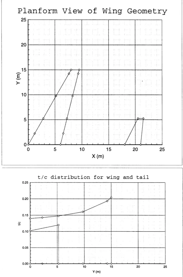
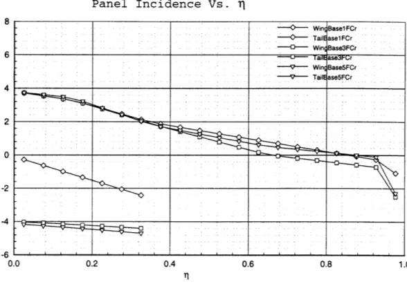
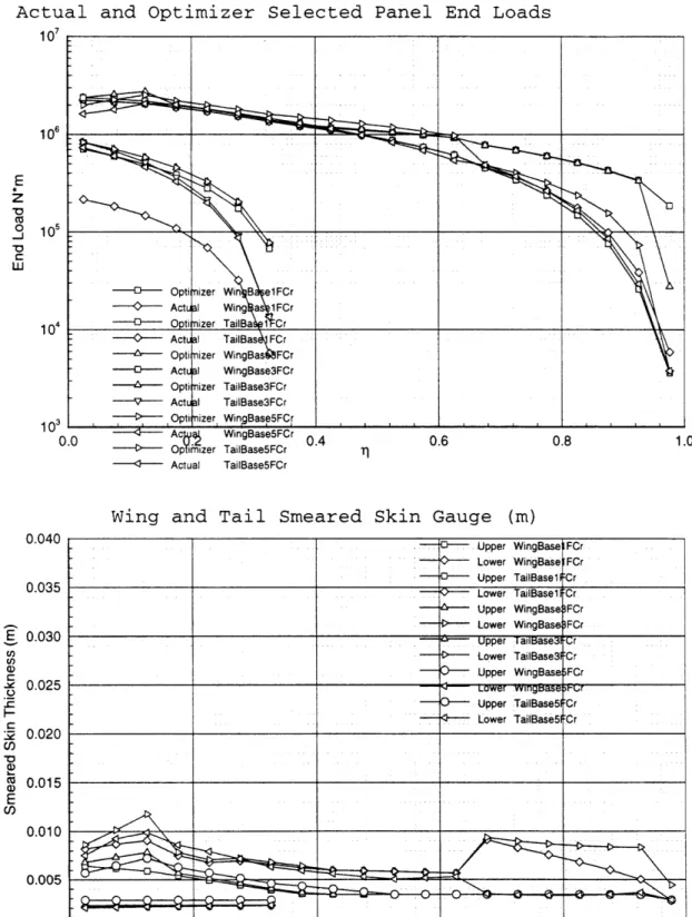
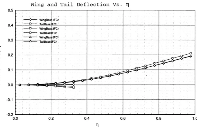
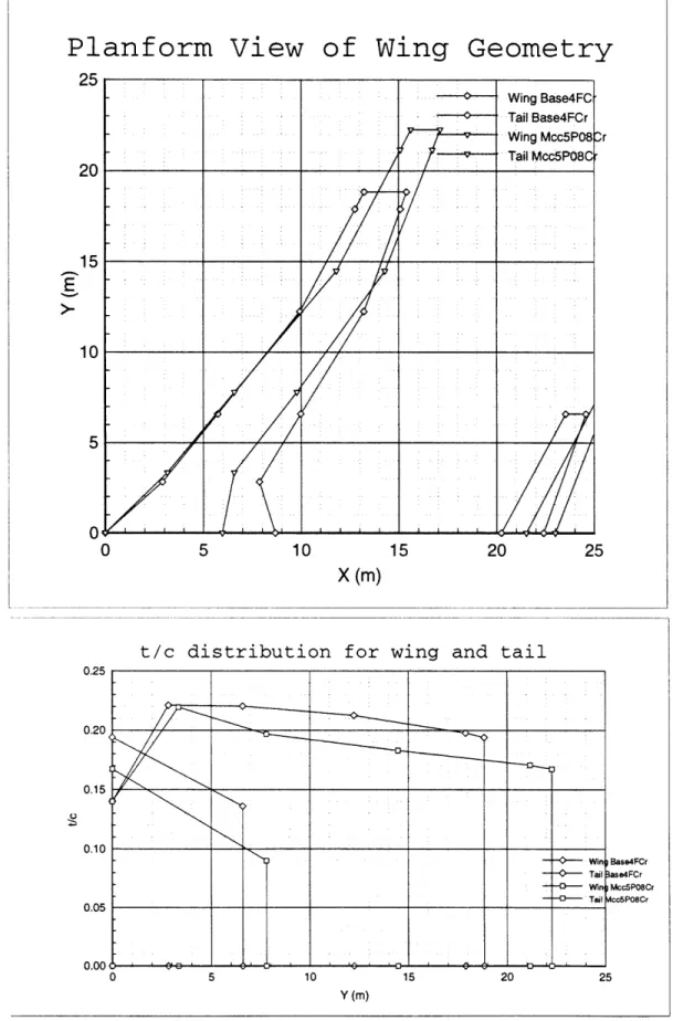
4.2 Plots Description ... . ... 44
4.2.1 Data Table Description ... 46
4.3 Baseline Aerodynamic Optimization Discussion . ... 47
4.3.1 First Optimization Changes ... 47
4.3.2 Final Planform Changes and Performance . ... 49
4.4 Default Drag Models ... .. ... . 56
5 Trade Studies Performed with the Code 59 5.1 Airfoil pitching moment Cm0 . . . 59
5.2 Upper to Lower skin maximum stress ratio . ... 60
5.3 Material density ... 60
5.4 Skin Roughness (% skin friction drag) ... .. 61
5.5 Effect of Wave Drag ... ... ... 62
5.6 Desired Cruise Mach Number ... 62
6 Trade Studies Results 63 6.1 General Comments on Trends in the Results . ... 63
6.1.1 Key to the Trade Studies Plots ... 64
6.2 Error Bars ... .... ... 66
6.3 Optimizer Bifurcation ... 67
6.4 Coefficient of Pitching Moment ... ... 68
6.5 Skin Stress Ratio ... 70
6.5.1 Stress Ratio Structural Parameters. ... . . . . 73
6.5.2 Aerodynamic Parameters ... 74
6.6 Wing Material Density ... .... ... 74
6.7 Effects of varying the Skin Roughness Parameter . ... 75
6.8 Crest Critical Mach Number Offset ... .... 78
6.8.1 Geometry ... . ... .. 79
6.8.2 Performance Parameters ... 80
6.9 Cruise M ach Number ... ... .. 81
6.9.1 Planform Analysis ... ... .. 81
6.9.2 Wing and Tail Geometry analysis ... . 82
6.10 Data Tables and Figures ...
83
7 Conclusions and Recommendations
119
7.1
Summary of Trade Studies ...
119
7.2 Importance of Static Margin ...
121
7.3 Problem M odeling ...
122
7.3.1 The other half of the issue: posing the optimization problem . . . . 123
7.4 Future W ork ...
.. ...
...
123
7.5 Conclusions . . . .
123
A Range Calculation
124
A.1 Fuel used in climb ...
125
B Foil Properties Scaling Derivations
126
List of Figures
1-1 Sample starting planform with elements and panels labeled . ... 18
1-2 WASP Structural Sizing Flow Chart ... 19
2-1 Plot of stress ratio vs. skin gauge ratio at several locations along the span starting at the root for parabolic skins ... .. 35
4-1 Baseline Starting Geometry ... ... 50
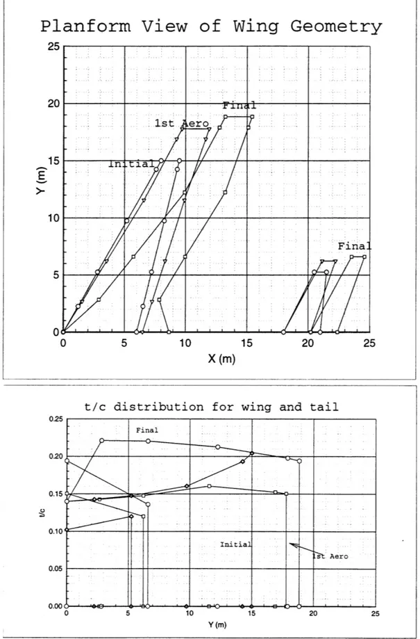
4-2 Baseline Optimization case; starting guess, one aerodynamic optimization and final planform ... 51
4-3 Baseline Optimization case; aero data for initial guess, one aero optimization and final design ... ... 52
4-4 Baseline Optimization case; aero data for initial guess, one aero optimization and final design ... ... ... ... 53
4-5 Baseline Optimization case; aero data for initial guess, one aero optimization and final design ... ... .. ... 54
4-6 Baseline Optimization case; aero data for initial guess, one aero optimization and final design ... 55
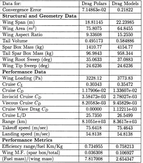
4-7 Baseline Optimization second aero iteration with Drag polars and Drag models 58 6-1 Comparison of C profiles for take off and cruise at small and large Kf values 65 6-2 Spar Box Weight Vs. Stress Ratio for fixed planform structural optimization 72 6-3 Skin stress ratio and thickness ratio relationship . ... 73
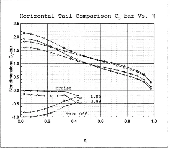
6-4 Effect of enforcing a down loaded tail with Static margin on the wing and tail planform ... ... ... ... ... 82
6-5 Trade Data for geometric parameters with variance of Cmo . . . . 85
6-6 Trade Data for performance parameters with variance of Cmo . . . 86
6-7 Planform data for Cmo = 0, -0.015, -0.04 and -0.10 . ... 87
6-8 Aerodynamic data for Cm0 = 0 , -0.015, -0.04 and -0.10 . ... 88
6-9 Trade Data for geometric parameters with variance of Stress Ratio . . . . 90
6-10 Trade Data for performance parameters with variance of Stress Ratio . . . 91
6-11 Planform data for Stress Ratio = 1.27 1.34 1.40 1.46 . ... 92
6-12 Planform data for Stress Ratio = 1.27 1.34 1.40 1.46 . ... 93
6-13 Skin data for Stress Ratio = 1.27 1.34 1.40 1.46 . ... 94
6-14 Trade Data for geometric parameters with variance of material density . . . 97
6-15 Trade Data for performance parameters with variance of material density 98 6-16 Planform data, short span, material density as independent variable . . . . 99
6-17 Planform data, long span, material density as independent variable ... 100
6-18 Aerodynamic data, short span, material density as independent variable . . 101
6-20 Trade Data for variance of skin roughness parameter . ...
103
6-21 Trade Data for geometric parameters with variance of Kcf ...
104
6-22 Trade Data for performance parameters with variance of Kcf ...
105
6-23 Planform data for Kcf
=
0.98
,
1.02, 1.03 and 1.04 . ...
106
6-24 Planform data for Kcf
=
0.98
,
1.02, 1.03 and 1.04 . ...
107
6-25 Trade Data of geometric parameters for variance of crest critical Mach
num-ber offset . . . .
. . . .. . .
109
6-26 Trade Data of aerodynamic parameters for variance of crest critical Mach
num ber offset . . . .
110
6-27 Planform data for Mcc
=
0, 0.03, 0.06 and 0.14
. ...
111
6-28 Planform data for Mcc
=
0, 0.03, 0.06 and 0.14
. ...
112
6-29 Trade Data of geometric parameters for variance of Cruise Mach number .
114
6-30 Trade Data of aerodynamic parameters for variance of Cruise Mach number 115
6-31 Planform data for Cruise Mach
=
0.675, 0.7, 0.75 and 0.85 . ...
116
6-32 Planform data for Cruise Mach
=
0.675, 0.7, 0.75 and 0.85 . ...
117
List of Tables
4.1 geometry and weight summary data for Baseline case structural sizing and
low speed optimization runs ... 45
4.2 Baseline Case data for Initial guess, after first aerodynamic optimization and the final optimized design ... ... ... 48
4.3 Baseline Case with drag polars and Similar case with code drag models, Mccoffset 0.08 ... ... .. . ... ... 57
6.1 Statistical error information ... ... 67
6.2 Comparison between the final planform for Cmo=-0.1 and the same planform run with Cmo=0.0 ... . ... ... 70
6.3 Component Drag Data for Skin Roughness coefficient trade study ... 76
6.4 Component Drag Data for Mcc Offset coefficient trade study . ... 79
6.5 Trade Data for variance of Cmo . . . . . . . . ... 84
6.6 Trade Data for variance of skin stress ratio . ... 89
6.7 summary data for p 2600, 2825, 2850, and 3000 4 . ... 95
6.8 summary data for p 2700 2750 and 2900 4 ... 96
6.9 Trade Data for variance of crest critical Mach number offset ... . 108
Introduction
The purpose of computing is insight, not numbers - R. Hamming
Aircraft wings are complex structures which need to be strong yet light, with low drag in cruise, yet able to fly slowly enough to land safely. The design of an optimum wing is inevitably a set of compromises. This problem would seem to be a prime candidate for com-puter optimization. However, there are two primary complications: planform optimization is a nonlinear problem, and constructing accurate but fast models for the optimizer is very difficult.
For a fixed planform, the approach to optimizing planform variables such as twist distri-bution, is linear and relatively fast. However, once the optimizer is allowed to vary the wing planform by modifying span, sweep, aspect ratio, the problem becomes nonlinear. While several nonlinear optimization algorithms exist, the mathematics are considerably more dif-ficult than simple linear analysis. This thesis is based on the Wing Aero and Structures Program (WASP)[1] written at Stanford. The optimizer chosen for the code is Sequen-tial Quadratic Programming (SQP) which attempts to strike a balance between speed and
stability. 1
The second problem is that a detailed computer model of any one aspect of wing design can take hours or sometimes even days to run a single simulation. During an optimiza-tion run, these models may be called several thousand times before finding a satisfactory optimum. In order to obtain a run time of less than a week, only simple models for the aerodynamics and the structure of the wing may be used. Short turn around time is espe-cially important because a code run is never perfect. Variables need scaling, minimum step sizes need adjusting, initial guesses need improvement, constraints need adjusting, and so even a full planform optimization code is still an iterative process.
Thus the models need to be fast, but at the same time, they must be able to accu-rately model the physics involved with the large number of design variables which affect the optimum design point. Of course, the optimizer knows nothing of airplanes and the optimum is simply wherever the optimizer finds the best "performance" out of these mod-els. If the models have holes or don't accurately reflect the physical processes involved, the optimizer will happily exploit these weaknesses and produce a completely unrealistic wing. Constraints may be applied to keep the optimizer from straying too far off track, but too many constraints limit the ability of the optimizer to find any sensible minimum.
Despite all the drawbacks, the process of multidisciplinary optimization of a full wing planform is an intriguing one which promises to offer new insight into the planform op-timization problem. At the current time, the WASP program is the most comprehensive single code written with the intent of optimizing the entire wing and tail planform in one big whack. Simple aero and structural models are combined with a gradient based optimizer which satisfies constraints over a combination of up to 14 flight conditions while searching
for a minimum, usually either minimum weight or maximum C. Available design variables
include the quarter chord sweep, wingspan, incidence angles, tail moment arm, and thick-ness distribution among others. The aero model is based on a simple lifting line method with enhancements to add in high lift, viscous and wave drag effects. The structural model
1
A commercial version of the quadratic optimizer called NPSOL and marketed by Stanford is commonly
used by industry for nonlinear optimization problems. The WASP version of the optimizer was written with the same algorithms but modified convergence criteria [1, A.5]
was based on a single cell beam which was sized according the the worst case of bending stress or buckling. There were also enhancements to find leading and trailing edge weights. The initial work on this code was done during an internship at the BOEING Company. Naturally, BOEING was only interested in the code if it could first duplicate their current deign codes and methodologies. Thus, the focus of the work during that period was an attempt to modify the existing structural and aerodynamic models in order to get better agreement with BOEING codes. Chapters 1 and 2 will describe in detail the code models and the modification made, in particular to the structural model.
BOEING was also interested as to whether the code could be sufficiently modified from
an "academia in-house code" to a production engineering code. The "user interface" for the code is somewhat cryptic, but much more of a problem for trying to package the code for general consumption is the actual optimization process. Unlike linear optimization algorithms which either converge or don't, nonlinear algorithms have a large nebulous zone in the middle. As will be explained in 1.3, the way a nonlinear optimizer deals with design variables and constraints is quite different from a conventional optimizer. Also, the choice of design variables, variable scaling, and minimum variable step size become critical to finding a good optimization path. The result is that it is not possible to simply plug in a starting planform and set of desired flight conditions and turn on the optimizer. Many code runs and re-runs are required to find the correct weights, scalings and combination of design variables and constraints to finally produce a well converged result. To even approach "packaged code" status for design engineering would require large amounts of pre and post-processing routines to prompt the user, and the results would still be quite questionable if the user was not familiar with the optimization process.
This thesis is based on applications of the modified WASP code (using the modifica-tions done for BOEING). A solid baseline optimization case was set up and tested to a satisfactory convergence. This case was then used as the starting point for a series of trade
studies on various aerodynamic parameters such as the airfoil Cm0, and the mach drag rise
point of the foil (wave drag). These parameters were given a range of values around the baseline value and then the full optimization procedure (a total of 6 passes at the optimizer) is run again.The set of final planforms were then analyzed to look at the quantitative and qualitative effect that parameter had on the optimized planform. Also of interest was the sensitivity of the design to the tested parameter.
Chapter 1 will present an overview of the code, SQP optimization, the code models, the flight conditions used during optimization, and a discussion of the code's assumptions and limitations. Chapter 2 goes into detail on the new structural model. Chapter 3 will discuss the step by step optimization procedure, the design variables, used, and the importance of variable scaling. Chapter 4 presents a detailed description of the optimization of the baseline case starting from a generic "initial guess" wing planform. Chapter 5 will discuss the trade studies done for the thesis, the parameters varied, why the parameters were chosen and any code related problems with those parameters. Chapter 6 will present the results of
Nomenclature
Note: Abbreviations for coefficients such as CDand Cdfollow the convention that a capi-tal subscript indicates a three-dimensional flow coefficient while the lower case subscript indicates that the coefficient is for two-dimensional flow.
a wing angle of attack in degrees from zero lift line
6 horizontal tail angle of attack in degrees from zero lift line
Co coefficient of drag (planform)
CD, inviscid drag coefficient
CD,,,o total coefficient of drag (includes all contributions from viscous, inviscid and com-pressible drag)
CD,, viscous drag coefficient
CDo compressible drag coefficient
Cd section drag coefficient
Cf flat plate turbulent coefficient of skin friction
CL coefficient of lift (planform)
L lift to drag ratio
CD
C, section lift coefficient
C, non-dimensional section lift coefficient (see equation 4.1 for the definition )
Cm0 airfoil section zero lift coefficient of pitching moment
Cm section coefficient of pitching moment
CmI section coefficient of pitching moment perpendicular to the sweep axis of the wing
cimax Maximum section coefficient of lift
Ix area moment of inertia around x axis
Ixz cross area moment of inertia, x and z axis
Izz area moment of inertia around z axis
Kcf flat plate Cf multiplicative factor to account for surface roughness
M.. free stream Mach number
Mcc Mach number at the thickest portion of the airfoil, the "crest critical Mach number"
Re Reynolds number
ay Skin stress in Pa, y direction (along the wing span from bending loads)
t airfoil geometry thickness to chord ratio
C
Chapter 1
Code Description and Overview
This Chapter will present an overview of the wing planform design problem and the "Wing and Aero Structures Program" (WASP) used for this thesis. Practical and theoretical aspects of the code will be discussed including, the optimization algorithm, the physical models, and the flight conditions used for optimization. The chapter closes with a discussion of the potential capabilities and limitations of the code.
1.1
Problem Definition
As was stated in the introduction, optimization of an aircraft planform is inevitably a set of compromises. There are a large number of design variables and an even larger number of constraints. The conventional method for design optimization is to pick one of these design variables and leave all others constant. The "independent variable" is tested over a range of values with the goal of finding a curve showing an optimum point. While each variable is being tested, all other variables are left fixed so as the isolate the effects of the independent variable. This approach has the benefit of being very controlled with a clear input and output. However, the method shows several disadvantages when it comes time to apply these isolated studies towards a full planform. Once a set of parameters has been tested in this way, it is up to the designer to figure out how to combine all the optimum curves. Some of them will most likely conflict and so decisions must be made as to which parameter is compromised. The design is modified and the process repeated. However, since changing one parameter in a vacuum is generally not realistic, the modified design will not be an optimum either and so the whole cycle iterates until time, budgets and design engineers are exhausted.
The solution to this of course is to simply take the entire design process and throw it at a super robust optimizer which can handle modifying all the design variables simultaneously to track down the final optimum planform. To a certain extent, this is what the WASP program attempts to do. However, as was also mentioned in the introduction, this approach has problems with modeling the problem well enough to get a good solution without needing weeks of computation time. The WASP code contains very simple models; a box beam for the spar and a lifting line for the wing. These are enhanced with numerical routines to provide for some low speed handling and compressible drag effects.
1.2
Optimization Code Procedures
There are three major sections to an optimization code: The optimizer, the physical models and the operating conditions. A short summary of each follows:
The Optimizer uses a set of design variables to create a "design space" which is an
n-dimensional map of the second derivatives of the goal with respect to each design variable. The optimizer takes steps in the direction of the steepest gradient until reaching a minimum. Constraints can be imposed to block off parts of the design space and impose outside conditions on the optimization.
The Physical Models are the mathematical representation of what is being optimized. In this case, lift and induced drag are by simple lifting line, the structures model relies on basic cell beam theory, and both models are enhanced to account for other factors, such as wave drag, flap lift and drag.
The Operating Conditions attempt to define the full envelope of performance demands on a wing and tail planform. Take off, climb out, cruise, maximum maneuvering load and other flight conditions are all applied to the design. Thus, while the optimizer may be attempting to minimize cruise drag, these conditions ensure that the wing will also be strong enough to maneuver, big enough to take off at a low velocity and otherwise satisfy all desired corners of the flight envelope.
Each of these sections can be written as a more or less independent code. To combine the three into a functional optimization routine requires one more section which controls what conditions and models are evaluated when and how this information is passed along to the optimizer. The next section explains the difference between "internal iteration" and "optimizer directed iteration" and presents an outline of the overall flow process through the code.
1.2.1 Code Flow Overview: Internal and Optimizer Directed Iteration
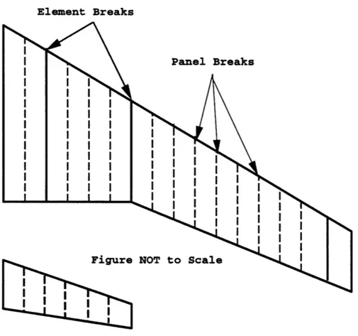
Optimization is a fundamentally iterative process. As the code starts, the existing condition is some starting guess, usually with constraints violated and lousy performance. Figure 1-1 shows an example of a starting planform with the elements and panels labeled. After an iteration the optimization process becomes a steady repetition of the following cycle:
1. Calculate the performance of the current planform at all required flight conditions 2. Find an optimization path based on improvement of performance and resolution of
violated constraints.
3. Take a "step" in this direction. This is accomplished by the optimizer picking new values for all of the design variables
4. If a step can not be found, check for convergence. If converged, exit. Otherwise repeat from step 1.
This is the outer optimization loop. Nested inside this loop can be numerous small iteration loops related to skin sizing, aerodynamic influence coefficients etc. The problem with these internal loops is that they also converge to some tolerance, with a convergence
Element Breaks
Panel Breaks
NOT to Scale
Figure 1-1: Sample starting planform with elements and panels labeled
derivative which can be significant and so are a considerable source of noise in the larger iteration scheme.[1, 3.3]
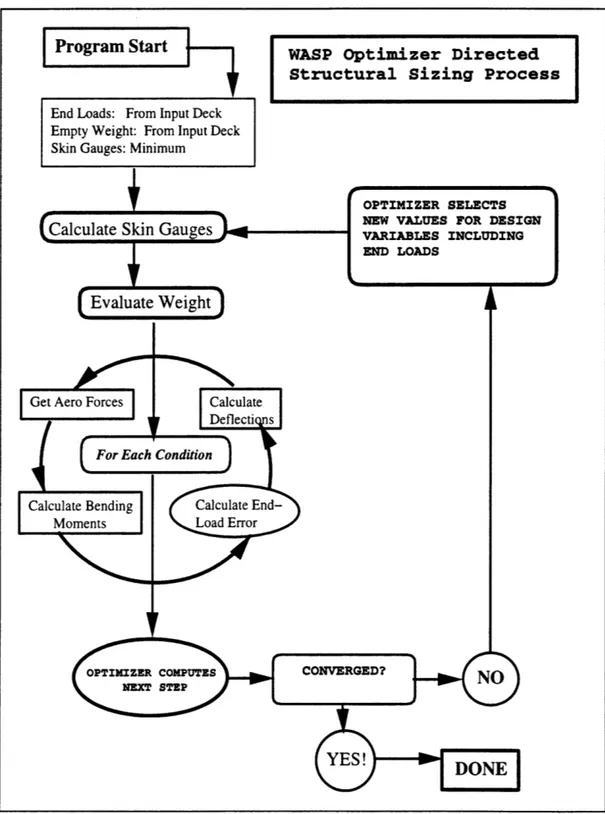
An alternative to nested iteration loops is to simply remove them. This is done by taking the variables from the internal loops and making them design variables which are then calculated in the outer optimization loop (optimizer directed iteration). This does remove the noise problem, but applying this approach to too much of the code would mean a large number of design variables and an even larger number of constraints. After some experimentation, it was found that the best approach was to make the structural design variables optimizer directed and leave the other internal loops [1, 3.3.2]. This leads to the introduction of an end load design variable for the root and tip of each element, where the end load is defined as: at, where a is skin stress and t, is the smeared skin gauge. Figure 1-2 shows a diagram of the overall code flow, and section 1.4.2 will detail the optimizer directed structural design process.
1.3
Fundamentals of Sequential Quadratic Programming
As with any optimization, the goal is to pose a problem which consists of a parameter to minimize, a set of design variables which will affect the minimization goal, and, if necessary, a set of constraints on the design variables. For example, a very simple optimization would be for minimum wing weight with a fixed planform. The optimizer would be allowed to adjust twist distribution, wing a and tail 6 and the wing skin endloads (structural design variables which will be explained in section 1.4.2 ).
Program
Start
WASP Optimizer Directed
Structural Sizing Process
Constraints could be placed on the maximum and minimum wing twist values as well as maximum allowable endloads. Other constraints to consider would be minimum skin thickness, maximum allowable deflection etc. The optimizer then takes the second order derivatives of the goal with respect to these design variables and constructs a design space. This space can be viewed as an "n-dimensional" topography in which the optimizer is searching for a local minimum. The constraints effectively serve to put boundaries on sections of the design space, or, to force the optimizer to find an optimum on the path of a specific constraint (for example: minimum weight for CL= 0.4).
Important Note: A linear optimization will first satisfy all the constraints, and then
optimize within these constraints. Thus, even a non-converged solution could still be within the constraint bounds. However, with non-linear optimization, the optimizer will work on improving the most active constraint while moving towards the goal. In the process, the optimizer will make sure that any other active constraints don't get worse, but won't actually work to improve the other constraints until they in turn become most active. Thus, if the optimizer hasn't found a fully converged solution there are probably several active constraints remaining.
1.3.1 SQP Specifics and Procedure
This section is distilled down from [1, Chapter 3]. The basic elements in the optimization
are the matrix of constraints, matrix of design variables, Hessian matrix, and the Lagrange multipliers. The Hessian is an approximate second derivative matrix based on information computed over the course of several iterations. The second derivative of the goal with respect to the design variables forms a gradient design space which the optimizer will use to find a step towards the local minimum. (Note: this means that the design variables must be second order smooth.) The optimization then proceeds in this sequence:
1. Initialize Hessian to identity matrix, compute the objective and the constraints from the current location.
2. Find a step to satisfy constraints
3. Use the SQP methods to find a step direction towards the goal
4. Execute a line search in this direction in order to minimize a merit function.
5. Depending on the success of the line search algorithm the code will now either re-set the Hessian and start from step 2, or continue by calculating the difference gradients. 6. Update the Hessian. If the new approximation is not positive definite, reset the
matrix to the I matrix. If the matrix is positive definite but doesn't pass a more strict check, the updates are bypassed. The newly calculated point now becomes the current location.
7. When the optimizer can no longer find improvement, check for convergence and exit
if converged.
The merit function checks the relative improvement in satisfying constraints through a summation of Lagrange multipliers, constraints at the present location and constraints at the projected location. See [1, section A.7] for details.
Convergence is checked for with the following formula:
Aact 0 A cact - C
Where Aact are the gradient constraints in the working step, A are the Lagrange
mul-tipliers, I is the identity matrix, p is the step vector, g is the objective gradient and c and
Cact are vectors of working constraints. Since the optimizer is required to set the Hessian
to the I matrix before checking for convergence, the I takes the place of the approximate Hessian. The Kuhn-Tucker conditions for convergence are:
-p = g+A A (1.2)
Which means that ideally at convergence the Lagrange multipliers are 0 and there are no more steps indicating that the minimum has been found.
1.3.2 Optimizer Design Space and Variable Scaling
The quadratic optimizer works by constructing a "design space" which is an n-dimensional surface composed of the second derivatives of the goal with respect to the design variables. In order for this approach to yield good results, all variables in the design space need to be scaled to be of order 1. If the variable slope is to small, the optimizer will have difficulty in finding a step on the shallow gradient. If the variable slope is too large, the steep slope will obscure other variables and alter the step direction. For a variable which directly affects the goal, this scaling should be calculated from the second order derivative. For the indirect variables, which are variables which do not directly affect the goal but which influence constraints, the scaling is a bit more complicated and needs to be done with the Lagrange multipliers. [1, p 69].
The constraints also have a scale factor, however this factor is much less critical than the design variable scaling. In this case, the scaling acts more like a weighting factor increasing or decreasing the penalty for violating that particular constraint.
The importance of the design variable scalings and step sizes can not be over emphasized. On a full optimization run there are 50 to 60 design variables and on the order of 600 constraints. Very rarely does the optimizer actually find a fully converged solution. Much more often the final solution is when the optimizer can not find another search direction and quits. If the error is small enough at this point, the code is called done. One of the factors output at this point is which particular design variable could not be improved. By modifying the scaling and or step size of this variable and re-running the last stage of optimization, the solution will often advance several more steps which can lead to significant changes in wing weight and less significant changes in the wing span, sweep etc.
1.4
Original Code Models
The primary physical models are the structural model for wing weight calculation and the aerodynamic model which uses lifting line and Treffetz plane to calculate the primary lift and drag. A full airplane wing consists of considerably more than a spar box and a set of horseshoe vortices. However for a lot of the calculations, these simple models will adequately represent the physics of the problem. The structural model can be enhanced with
multiplicative factors to take into account "other weight" such as high lift systems, access hatches etc. Much more difficult to model and not included in the code is additional weight necessary to eliminate flutter. A simple aerodynamic model is only a valid approximation to a wing at cruise, and the validity of lifting line on highly swept wings is also questionable. The code needs to account for wave drag, flap and slat drag, flap and slat lift, and viscous drag so these are patched in with empirical functions which are sometimes built into the code and sometimes user input.
1.4.1 Original Structural Model
The structural model was changed significantly from the original WASP code. This section will give a summary of the original model and the problems found. The next section will summarize the changes made and chapter 2 will go into detail on the new structural model. For a complete description of the original structural model, see [1, sections 2.2,2.3].
1.4.1.1 Model Assumptions
The WASP code is meant to size just about everything on the wing including -, chord, dihedral and sweep. If all of these variables were treated independently, the code would gain significant complexity in variable storage and handling. A better approach for this level of design is to find a way to scale and modify a basic wing cross section over the full length of the wing. This approach requires several major assumptions:
1. There is only one generic airfoil cross section
2. The upper and lower skins of the spar box can be represented by parabolas fit to three points which were supplied by the user.
3. The smeared skin gauge is constant around the foil so that once the inertial properties,
Ixx, Izz, Ixzare calculated, they can also be scaled to the local land chord.
4. This airfoil can then be scaled to fit local land chord.
5. The maximum or minimum z coordinate with reference to the z centroid is the location of maximum stress and sizes the wing skins.
The assumption that there is only one foil cross section for the entire wing is not valid aerodynamically, but from a structural standpoint, the variations in the actual spar box dimensions can be kept quite consistent along the wing so this approach is reasonable. Likewise, the skins over the length of the spar box are relatively flat so a parabolic approxi-mation is reasonable. Carefully picking which three coordinates the curve will be fit on can help improve this approximation.
The constant smeared skin gauge all the way around the spar box is not a valid assump-tion. In almost all cases, the spar box is sized by bending, and bending is driven by Ixso that the upper and lower skins offer most of the resistance to bending in the vertical plane, while the front and rear spar make almost no contribution (in this direction). Thus, a spar box with this assumption will end up significantly heavier than necessary. See section 2.2 for a description of the fix applied to this problem.
From an aerodynamic standpoint, supercritical foils do not scale simply with c. Instead, the airfoil is changed to match scaled pressure distributions. However, the code is already
assuming a single airfoil cross section and so the geometry behind scaling the structural properties can be worked out. This can actually be a bit tricky and and is derived in appendix B.
1.4.2
Skin Sizing by Optimizer Directed Iteration
Bending, Shear and Torsion moments are all calculated along the length of the wing. The skins are then sized to by the most critical of these loads. At this point the integration with the optimizer starts to become apparent. As was briefly mentioned in 1.2.1, the skin sizing problem has been placed in control of the main optimization loop. The function takes the current end loads from the optimizer and sizes the skin gauges to withstand the load simply by constraining the calculated structural end load to be less than the applied end load. There are two end loads for each element, one for the root and one for the tip. These are design variables which are always necessary when the optimizer is sizing the structure. The optimizer directed iteration makes the skin sizing process proceed as follows:
1. Initialize the skin to minimum gauge 2. Calculate foil properties (I,,etc.)
3. Call the function to size the skin gauges and then calculate the resulting wing weight. 4. Call the aerodynamic models to calculate the lift and drag forces
5. find the resulting bending moments
6. Use the bending moments to find the actual end loads on each element. 7. compare these end loads to the end loads the skins were sized with in step 3
8. Use constraints to force the optimizer end loads to be greater than the actual calcu-lated end loads
9. Based on the violated constraints, the optimizer picks a new set of end loads. 10. repeat
This is diagrammed in figure 1-2. This approach to skin sizing works quite well most of the time but will occasionally produce very heavy wings. Constraints are applied to make sure the optimizer end loads exceed the actual end loads which keeps the wing from failing. However, making a structure twice as strong as necessary will satisfy the constrains just fine while carrying around a lot of extra weight. The optimizer is quicker to satisfy constraints than to shave off weight. Constraining the end loads to be very close to the actual end loads (not just greater than) will make for very shallow gradients in optimization space and the optimizer will have difficulty finding a search path. The result is that the wing will sometimes end up with some extra structure, especially in regions of discontinuity (sweep or taper change).
In the original MassEval function the skin gauges are calculated using a number of buckling equations which had been solved for skin gauge. The optimizer end loads were used in the calculation and the resulting skin gauge was then multiplied by the scaled unit area of the spar box and the panel width to get the volume of Al for that panel, and hence
skin thickness sizing. This set of criteria almost always defaulted to the bending load as the most critical. For that matter, since the spar box had assumed constant smeared gauge on all sides the code would be unable to re-size the shear webs to resolve a torsional wing sizing problem. This approach would generally find a reasonablel skin thickness. However, applying the same thickness to the entire spar box would result in a total spar box weight several times higher than necessary. Chapter 2 will give a detailed discussion of the new weight model implemented to solve this problem.
1.4.3 Other Structural Parameters
The code calculates a Structural Influence Coefficient matrix for bending and twist, and
also takes into account aeroelastic effects. These models were given a standard
BOE-INGplanform as a validation test. The aeroelastic effects came out quite well, however the
wing deflections under load were about ! of the BOEINGdeflections. The routines which did these calculations were not changed so this holds true for all cases done in this thesis.
1.4.4 Weight Calculation
There are three major components to aircraft weight: Structural weight, fuel weight and all other weights.
Structural weight This is the weight calculated from the wing and spar boxes when sized to meet all structural design loads. Using the new weight method, the spar box structure is modeled as four skins with parabolic upper and lower skins and vertical webs. The webs stay at a pre-set thickness, while the optimizer varies the upper and lower skins to meet design loads. The effect of stringers is incorporated into the wing by using a "smeared skin gauge" which is the average thickness of the skin and stringers combined.
Fuel weight The fuel weight is the difference between the Maximum take off weight and the maximum zero fuel weight. Both of these parameters are user entered and are constant. Thus the fuel mass is constant and the optimizer will have to design a wing to contain the desired fuel volume. The relevant variable here measures the fraction of total available fuel volume actually occupied by fuel. This is constrained to < 1.
Other Weights There are actually 3 sub-categories of this section, calculated, scaled and
flat weight. The only calculated weights were the leading and trailing edges which were sized to withstand a fixed pressure load [1, Section 2.3.7]. These weights were not considered necessary for the purpose of this study and the pressure loads were left constant for all cases.
The scaled weights were simply empirical factors multiplied by the wing area to get various add-on weights such as inspection hatches, rib to spar joint weights etc. These factors only add an offset to the final weight and do not affect the design in any way. Flat weights are simply for anything else the user wants accounted for in the total weight. Major items include landing gear and fuselage, both of which were set to zero. If the engines were on the wings, the code did have provisions for attaching a fixed
"'Reasonable" as defined by comparing the output of WASP with BOEINGpreliminary design codes.
mass on a specific wing panel to simulate the engine. The effects of engine thrust on wing structure would not be included.
1.4.5
The Aerodynamic Model
The aero model is a simplified version of LINAIR, which is a vortex lattice code written
by Professor Ilan Kroo.
2In WASP, a single lifting line at the quarter chord is used for lift
calculation with induced drag calculated in the Treffetz plane. This code does model the full
wing to allow for asymmetric effects of aileron deflection. However, there is no correction
for a fuselage and lift is assumed continuous across the center of the wing. Another problem
is that the panel widths in WASP tend to be quite large, on the order of 1 meter in width.
This makes it very difficult for the code to accurately model the lift towards the wing tip
where the lift distribution is changing very quickly.
1.4.6
Drag Calculations
The original code had three options for calculating CD,and a fourth was added for use at
BOEING. These applied during cruise and additional corrections are necessary when using
the high lift devices for take off and landing as will be briefly explained in section 1.4.7. The standard method for finding CDois to use the local Renumber to calculate the flat plate turbulent skin friction coefficient (Cf).
0.455
Cf = Kf 0R)2.584 (1.3)
(log 0Re )2 58 4
where Kf is a multiplicative constant to account for "surface roughness". This was set to 1.0 for most code runs. The other two methods depend on user inputs. The first asks the user for an array of Cfvalues to use instead of calculated values. The second asks the user for the first and second order coefficients for a C,- Cddrag polar.
To increase the accuracy of finding both CD, and CDc, the ability to reference user input drag polars was added. The user enters as many polars as desired along the wing span. The code then interpolates and scales the polars to local !as described in appendix B. During aero model evaluation, the code scales the polars to account for local sweep and Mach
number. Polars from a generic BOEINGairfoil3 for a small transport were used for most
of the code runs done in this thesis.
The rest of the parasite drag for the aircraft (nacelles, fuselage, etc.) is accounted for with the user input ffus parameter, which is an equivalent drag area. This scales as:
CDf =
fus
(1 + 0.38C2)SrefL
Where the 0.38 is a purely empirical correlation, again for a small transport[l, page 44].
NOTE: For this thesis, the CDfu, was left at zero.
2
Professor Ilan Kroo teaches Aeronautics at Stanford University and was the thesis advisor for the WASP program
3
1.4.6.1 Wave Drag
The Wave Drag model uses the Shevell Crest Critical Mach Number, Mcc method[1, section 2.4]. This method determines the minimum Mach at which supersonic flow would occur at the thickest point of the foil:
M
Mseparation = [known value] > + MCCf (1.4)
MCC + MCCoff set
Simple sweep is then used to correct Moto M1 . The Mcc is a function of tand CL. Drag
is found from an empirical correlation [1, figure 2.16]. The attractive part of this model is that it is quick and changes with !so that the optimizer will have to balance !based on drag and weight. However, in validation tests, the drag tended to be excessively high.
1.4.7 High Lift Devices
A lifting line model does not predict stall behavior or separation drag, therefore the aerody-namic model needs a set of adjustments to handle the effects of the high lift devices during take-off and landing. The code needs to be able to predict the wing stall speed, stall a, maximum lift clean wing, and maximum lift with high lift devices.
Clean Wing Stall Is found from the lifting line model and the user input CLm,, for each
element. When any one panel is determined to be at CLm,,, the wing is stalled
Lift From Flaps and Slats As explained in [1, section 2.5.2], the extra lift and increased
CLmax from the flaps is calculated using CLincrements multiplied by the flap deflection
angle. The actual maximum lift is found by calculating an equivalent panel incidence increment and adjusting the lifting line accordingly so that maximum lift and stall can be calculated as in the previous method. Lift from slats is also an empirical adjustment. [1, section 2.5.3]
Drag for the high lift devices is purely empirical. A drag increment is added to the total
CDfor flaps and slats. The slat calculation is very simple - when the slat is down, add .006
to the total CD. The flaps are very slightly more sophisticated with the drag increment depending on the flap deflection angle. [1, pp 47,48]
1.4.8 Flap Induced Flow Corrections
One item which is treated in some detail in the thesis is the application of an incidence correction to the panels which border panels which have flaps deployed. Since the flaps modify the incidence of the neighboring panels, and thus the stall a of those panels, the critical section approach to maximum lift could be in error if this effect is ignored. The
computed correction depends on local geometry, C1 and a set of empirical correlations
calculated in LINAIR (in full Vortex Lattice Mode) [1, pp 51-56].
1.5
Flight Conditions
There are a total of 14 available flight conditions which can be used for the planform optimization. Each condition has a number of attributes which can be set by the user. These include the options which should be calculated for that flight condition (high lift
drag, compressible drag and other options), the operating conditions and some geometry
factors. For example, at the take off condition, the altitude, velocity, load factor, slat and
flap deflections, slat CLincrements, and aileron deflections can all be specified with the
options including "calculate high lift drag and proximity to stall". The take off condition
also has pre-defined attributes in the code regarding the need for the elevator to rotate the
fully loaded aircraft to take off and trim to climb out etc.
Definitions: MTOW
=
Maximum Take Off Weight and MZFW
=
Minimum Zero Fuel
Weight.
1.5.1 Structural Conditions
There are a total of six structural conditions. Usually the critical structural condition is the high load maneuver at MTOW. The abbreviation after each condition is the reference label used for that condition in the code.
1. Cruise at MTOW, aft CG (Cr )
2. Vertical Gust, forward CG, MZFW (Gt) 3. Horizontal Gust, forward CG, MZFW (Sd)
4. Maneuvering Condition forward CG, MZFW (Mn )
5. Maneuvering Condition forward CG, MTOW (Mf)
6. Another Cruise Condition at forward CG, MZFW (St)
1.5.2
Tail Sizing Conditions
The tail planform is designed simultaneously with the wing, which requires an additional
series of flight conditions. Generally the tail will turn out much too small unless the op-timizer has to meet requirements for maximum tail pitch authority. The conditions used primarily to size the tail and elevator are:
1. Take-off rotation, forward CG, MTOW (TO)
2. Landing Approach mis-trim. Condition assumes flaps down, 1.8 Vstai, stabilizer trim set for approach, and elevator only can be used to trim the aircraft. (sizes the elevator)
(FM)
Some of the other high lift conditions in the next section may also influence horizontal tail sizing.
1.5.3
High Lift Conditions
In order to size the wing properly for take off and landing several high lift conditions can be specified along with the desired flap and slat settings and speeds to try to fly.
1. Take-off Rotation (see previous section)
2. Take-off Maximum lift forward CG, MTOW, check stall speed (HL)
4. Landing maximum lift, forward CG, MZFW, calculate landing stall speed (FD) 5. Landing approach, forward CG, MZFW, 1.3 Vstau (from FD), sets trim setting for the
FM condition. (FA)
1.5.4 Other Conditions
The weight model includes the effects of inertial bending relief that wing fuel tanks supplies. The optimizer found it could take advantage of this by moving fuel outboard to the extent of trying to create tip tanks. To penalize this approach, a Taxi Bump (Tx) condition was added which is some load imposed with zero airspeed so the wing has to take the mass imposed bending moments.
The last condition, which is not critical to overall planform design, is the Rolling Moment
Check (HR). This condition is used to size the ailerons, usually to meet the maximum hinge
torque constraint. One visible effect of including this option is that the outboard wing trailing edge will have a reduced sweep in order to get the aileron hinge line closer to being perpendicular to freestream.
1.6
Code Assumptions and Limitations
The code was written for optimizing planforms for mid-sized subsonic commercial transports and should be applicable to aircraft in the 100-300 passenger range. Larger of smaller aircraft have changes in construction methodology which reduce the accuracy of the weight analysis.
The simple lifting line will not tolerate sharp breaks in chord along the span or other unusual geometries. Furthermore, there are internal code limits to the total number of panels which can be set for the wing, somewhere in the range of 35. Since the paneling is fixed width instead of a cosine distribution, the errors introduced at the tips of long, high aspect ratio wings become considerable. Also, the paneling in the tail must line up
exactly with any panels in the wing which the tail overlaps (due to the code methodology in
LINAIR).
The empirical increments used for the flaps and slats are only good for a fairly generic set of flap and slat deflections so more efficient high lift systems would be unnecessarily penalized.
The crest critical mach number method produced excessively high drag values when run with a standard aft loaded, highly cusped supercritical airfoil. The Mccoffset can be used adjust this drag down to much more reasonable values but finding the exact required offset is difficult.
The code does not model a fuselage, account for loss of lift in fuselage carry-over fashion or account for vortex drag at the fuselage-wing intersection. These parameters are sensitive to flight velocity and would affect planform outcome.
The use of drag polars allows a much more accurate drag assessment, but this is only good provided that the optimized planform has ended up quite close to the design the polars were originally meant for. Designs which stray too far from the original foil size and operating point will probably leave the valid range of the polar.
Chapter 2
Modifications to the WASP Code
Several modifications were made to the WASP code while working at BOEING. The addi-tion of drag polars to the list of methods for calculating CD, and CD, was a simple addiaddi-tion to the capabilities of the code. A correction was made to how the code handles the section Cmo. Major modifications were made to the skin thickness calculation part of the structural
model.
2.1
Pitching Moment Correction
During code evaluation trials at BOEING, the tail span loading profile was consistently
incorrect even though the wing spanload was reasonably accurate. In [1, B.2] there is a
lengthy discussion of how to handle the section pitching moments. The section describes two derivations for Cmo, one for a "swept wing" and the other for a "sheared wing". The results
of the derivation are that the "swept" case corrects with cos3A while the "sheared" case
corrects with a cosA (where A is the local quarter chord sweep). According to comments in
the code, this correction was intended to be applied to a Cm0 from a streamwise foil section.
Most Cmo data available is from MSES1 or similar programs and is Cm.. The following
equations are from Doug McLean [7] and are used in a pre-processing program that modifies
the MSES Cm1 to be a streamwise Cmo,,.
Definitions:
V = FreestreamVelocity Vector
c = freestreamchord
q = freestreamdynamic pressure
(2.1) Basic Conversions: to convert each of the above freestream values to the equivalent vector
perpendicular to the quarter chord:
VL = V Cos A
CI = CcosA
1MSES is a multi-element airfoil design optimization and analysis code written by Professor Drela at MIT
q± = qcos2A
(2.2)
CmoDefinition For the quarter chord pitching moment:
M_
Cm 4 (2.3)
SqSc
Using the above relations, the conversion is simply:
Me Cmc = q41 MS cos A 4 q cos2 ASc(cos A) Cm -= (2.4) cos2 A
And since the input data is the Cmj:
CmC Cm cos2 A (2.5)
and
M = CmC cos2 AqSc (2.6)
Cm
Which is obvious on inspection since Cm =
-s
and substituting this back intoequation 2.6 simply gives: M = CmqSc which is correct by definition. From [1, Section B.2] :
btan A
M = q cos ACrm c S + q cos2 C1 2 S (2.7)
The second half of the term is from the integration of the pitching moment across the
span of the wing and can be re-derived. The first term is also the same once the c1 is
converted back to c, and again, on inspection, the first term reduces to the definition of Cm. However, there seems to have been a disconnect between this section and the actual coding. The code expects a streamwise Cmo (according to comments in the code), and the chord was already streamwise, but the cos A term stayed in anyway. The code was changed to
use a cos2 A correction and so the Cm0 in the input deck should be a Cmj. This fix greatly
improved the agreement of the horizontal tail loading.
2.2
Spar Box Skin Sizing and Weight Calculation
The previous chapter contained a discussion of the optimizer directed iteration and the original code model. As was discussed in section 1.4.1.1 the original model made several simplifying assumptions which significantly reduced the accuracy of the weight predictions. This new weight model was written using BOEING preliminary design code structural methods as a guide. The intention was both to provide a more realistic spar box structure and try to match the output of BOEING preliminary design codes.
A number of attempts were made to completely change the structural model. However,
documentation on the code was very limited, as were time and resources. The initial
attempts to replace the skin sizing routine met with severe optimization instabilities and were abandoned. Eventually a new method was patched together that would work with the panel end loads which were the already existing design variables. However, since the previous structural model had assumed a more or less symmetric spar box with even skin thickness distribution, there was only one set of end loads for each element. Since it was desirable to optimize the upper and lower skins independently, a brief attempt was made to double the number of skin end load design variables. This also meant doubling the number of constraints, which is a much larger number since there is one constraint for each panel. The attempt also ended in optimizer instability problems and was abandoned. The following procedure was finally adopted as being the best method that could be applied with the existing design variables.
2.2.1
Background Information
The codes this method is based on requires the maximum material stress,
Uy
as a userinput. The method works by calculating the actual stress in the foil at several points
-usually the front and rear spars and the middle of the sparbox. The skin thickness is then corrected based on the ratio of actual to allowable stress and this process iterates until actual skin stress matches maximum skin stress. The maximum skin stresses are a user input parameter with one value for each element. In the WASP code the internal iteration has been removed so that for each time the optimizer calls the structural model, new skin gauges are calculated from the stress ratio and simply returned.
From Rivello [6, section 7.3] the governing set of equations for a box beam are:
_ P - -
~z
(2.8)S- A Iz-Izz - Iz z - z
(2.8)
The f term is for loads along the axis of the beam (loading a beam in compression) and is zero in this case.
2.2.1.1
Compression and Tension Allowables
There is an added complication to this method which is due to the fact that the maximum compression stress allowable in a material is a function of end load. The maximum stress under tension does not change with end load so these values can be entered in a short array in the input deck. However, a table of compression allowable vs. end load must be supplied for the calculation of skin thicknesses for surfaces in compression. The code will interpolate the maximum compression allowable from the existing end load. In case the end load falls above or below the limits of the table, the maximum value will be used. There is no extrapolation.
There was also insufficient time to tie in a torsional sizing model to calculate the thick-nesses of the front and rear spar webs. Instead of assuming a constant thickness these values have also been made a user input parameter. The web thicknesses used for this thesis were approximated from a similar sized transport wing[9].