Air Traffic Flow Management at Airports: A
Unified Optimization Approach
by
Michael Joseph Frankovich
B.A., University of Auckland (2008)
B.E., University of Auckland (2008)
Submitted to the Sloan School of Management
in Partial Fulfillment of the Requirements for the Degree of
Doctor of Philosophy in Operations Research
at the
MASSACHUSETTS INSTITUTE OF TECHNOLOGY
September 2012
c
Massachusetts Institute of Technology 2012. All rights reserved.
Author . . . .
Sloan School of Management
August 17, 2012
Certified by . . . .
Dimitris J. Bertsimas
Boeing Leaders for Global Operations Professor
Co-director, Operations Research Center
Thesis Supervisor
Accepted by . . . .
Patrick Jaillet
Dugald C. Jackson Professor
Co-director, Operations Research Center
Air Traffic Flow Management at Airports: A Unified
Optimization Approach
by
Michael Joseph Frankovich
Submitted to the Sloan School of Management on August 17, 2012, in Partial Fulfillment of the
Requirements for the Degree of
Doctor of Philosophy in Operations Research
Abstract
The cost of air traffic delays is well documented, and furthermore, it is known that the significant proportion of delays is incurred at airports. Much of the air traffic flow management literature focuses on traffic flows between airports in a network, and when studies have focused on optimizing airport operations, they have focused largely on a single aspect at a time.
In this thesis, we fill an important gap in the literature by proposing unified approaches, on both strategic and tactical levels, to optimizing the traffic flowing through an airport. In particular, we consider the entirety of key problems faced at an airport: a) selecting a runway configuration sequence; b) determining the balance of arrivals and departures to be served; c) assigning flights to runways and determining their sequence; d) determining the gate-holding duration of departures and speed-control of arrivals; and e) routing flights to their assigned runway and onwards within the terminal area.
In the first part, we propose an optimization approach to solve in a unified manner the strategic problems (a) and (b) above, which are addressed manually today, despite their importance. We extend the model to consider a group of neighboring airports where operations at different airports impact each other due to shared airspace.
We then consider a more tactical, flight-by-flight, level of optimization, and present a novel approach to optimizing the entire Airport Operations Optimization Problem, made up of subproblems (a) – (e) above. Until present, these have been studied mainly in isolation, but we present a framework which is both unified and tractable, allowing the possibility of system-optimal solutions in a practical amount of time.
Finally, we extend the models to consider the key uncertainties in a practical implementation of our methodologies, using robust and stochastic optimization. No-table uncertainties are the availability of runways for use, and flights’ earliest possible touchdown/takeoff times. We then analyze the inherent trade-off between robustness and optimality.
Computational experience using historic and manufactured datasets demonstrates that our approaches are computationally tractable in a practical sense, and could
result in cost benefits of at least 10% over current practice. Thesis Supervisor: Dimitris J. Bertsimas
Title: Boeing Leaders for Global Operations Professor Co-director, Operations Research Center
Acknowledgments
1I would firstly like to thank my advisor Dimitris Bertsimas, without whom this would not have happened. You always had a clear direction in mind. I admire your energy and greatly appreciate everything you have done for me. It has been a privilege working with you.
A special thanks is also due to Amedeo Odoni, a font of knowledge of the airline industry – thank you for your conscientious feedback, your kindness and your support. I would like to thank Mariya Ishutkina, Rich Jordan, Jim Kuchar, Tom Reynolds and Ngaire Underhill of MIT Lincoln Laboratory, as well as Professor Hamsa Balakr-ishnan for providing me with much of the data necessary to complete this thesis. I am also very grateful for the feedback and direction I received from many of the same, and also from Bill Moser and Mark Weber of MIT Lincoln Laboratory, Professor Cindy Barnhart, and fellow students Ross Anderson, Chaithanya Bandi, Shubham Gupta, and Phil Keller.
Thank you to all those who have made the ORC such a special place to be a part of over these past few years. To Andrew and Laura – thank you for all the work you put in for us – you really do go beyond what’s expected to make our lives easier, and it is much appreciated. To co-directors Cindy, Dimitris, and Patrick Jaillet, thank you for putting in your time and energy. Most of all, thank you to my fellow students and friends, I look back with great fondness upon the times we have shared.
To my Mum and Dad, I cannot adequately express my gratitude to you. Thank you for your love and support which has always been with me. Thank you to the rest of my family and friends for always being there, especially my wonderful sisters. Fi-nally, to Andrea, thank you for your unwavering love and support, I couldn’t imagine these years without you.
Cambridge, August 2012 Michael Frankovich
Contents
1 Introduction 19
1.1 Background and Literature Review . . . 20
1.1.1 Runway Configuration Management and Arrival/Departure Run-way Balancing . . . 20
1.1.2 Runway Sequencing . . . 20
1.1.3 Surface Management . . . 21
1.1.4 Airport Optimization under Uncertainty . . . 22
1.2 Contributions and Outline of Thesis . . . 22
2 Strategic Airport Optimization 25 2.1 Introduction . . . 25
2.2 A Mixed Integer Programming Model for a Single Airport with Con-stant Configuration Changeover Times . . . 31
2.2.1 Example Problem . . . 35
2.2.2 A Baseline Policy . . . 38
2.2.3 Computational Results for Larger Problems . . . 42
2.3 Multiple Changeover Times . . . 46
2.3.1 Size of the Model . . . 48
2.3.2 Computational Results . . . 48
2.4 Optimizing Over a Metroplex of Airports . . . 50
2.4.1 Multiple Airport Mixed Integer Programming Model . . . 50
2.4.2 Computational Results . . . 53
2.6 Summary . . . 56
3 Tactical Optimization of Air Traffic at Airports: A Unified Ap-proach 57 3.1 Introduction . . . 58
3.2 The Airport Operations Optimization Problem . . . 60
3.2.1 Data . . . 61
3.2.2 Decision Variables . . . 64
3.2.3 Objective Function . . . 64
3.2.4 The Binary Optimization Problem . . . 65
3.2.5 Valid Inequalities . . . 70
3.3 Phase Two – The Routing Subproblem . . . 73
3.3.1 Data . . . 73
3.3.2 Input from Phase One . . . 74
3.3.3 Decision Variables . . . 76
3.3.4 Objective Function . . . 76
3.3.5 The Binary Optimization Problem . . . 77
3.3.6 Valid Inequalities . . . 80
3.4 Computational Experience . . . 81
3.4.1 Model Validation and Computational Tractability . . . 82
3.4.2 Benefits Assessment . . . 84
3.5 Summary . . . 92
4 Optimization of Air Traffic at Airports in the Presence of Uncer-tainty 93 4.1 Introduction . . . 93
4.2 Incorporating Uncertainty in Flights’ Earliest Possible Touchdown/ Takeoff Times . . . 96
4.2.1 A Robust Optimization Approach . . . 97
4.2.2 Modeling Uncertainty to Determine the Robust Optimization Parameters . . . 100
4.2.3 Simulating a Stochastic and Dynamic Environment . . . 104 4.2.4 Computational Experience . . . 107 4.3 Incorporating Uncertainty in Runway Availability . . . 114 4.3.1 A Two-Stage Stochastic Robust Optimization Problem . . . . 115 4.3.2 Computational Experience . . . 120 4.4 Summary . . . 121
5 Concluding Remarks 123
A Separation Calculations 125
A.1 Separation Rules . . . 125 A.2 Data Used . . . 126 A.3 Separation Times Used . . . 126
B Configurations at BOS and DFW 129
List of Figures
2-1 A runway configuration used at BOS, with the corresponding active
runways indicated. . . 26
2-2 Runway configuration capacity envelopes (RCCE) for a single config-uration under VMC and IMC. . . 28
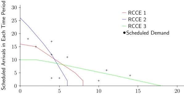
2-3 Test Problem 1 data, with 3 configurations and 15 time intervals. The scheduled demand is indicated for intervals 1 to 10, and is zero for intervals 11 to 15. . . 36
2-4 Test Problem 1 solution, intervals 1 and 2. . . 37
2-5 Test Problem 1 solution, intervals 3 to 6. . . 37
2-6 Test Problem 1 solution, intervals 7 to 12. . . 38
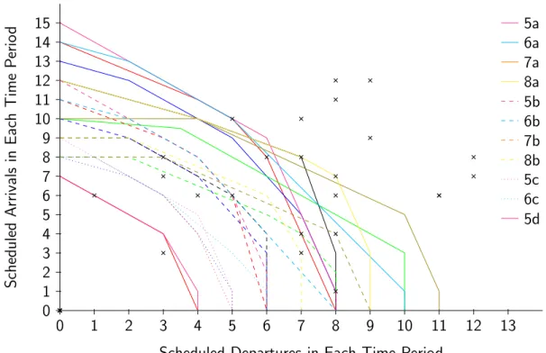
2-7 Test Problem 2, with 4 configurations, 11 RCCE and 30 time intervals. In the legend “2c” indicates the third RCCE for configuration 2, etc. 43 2-8 Test Problem 3, with 8 configurations, 22 RCCE and 30 time intervals. The colors and styles for Configurations 1 – 4 and their RCCE are the same as in Figure 2-7. . . 44
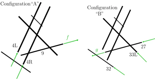
3-1 Example illustrating an element (f, g) belonging to the set Q at BOS. The arrows indicate the direction and mode of traffic as dictated by the configuration in use. Suppose in the solution to P3-1 we have: i) configuration A is used first, then configuration B, ii) flight f is assigned to runway 9, and flight g to runway 27. Since runway 27 is not used in configuration A, we have (f, g) ∈ Q. . . 75
3-3 Boxplot of P3-1 and P3-2 computation times for BOS. . . 85
3-4 Boxplot of historic and optimized surface times for departures at DFW, as well as optimized gate-holding. . . 86
3-5 Boxplot of historic and optimized surface times for arrivals at DFW, as well as optimized fix-delays (i.e. speed control before reaching fix). 87 3-6 Boxplot of historic and optimized surface times for departures at BOS, as well as optimized gate-holding. . . 88
3-7 Boxplot of historic and optimized surface times for arrivals at BOS, as well as optimized fix-delays (i.e. speed control before reaching fix). . 88
3-8 Contribution of scheduled flights in the optimization time window to surface congestion at DFW. . . 90
3-9 Contribution of scheduled flights in the optimization time window to surface congestion at BOS. . . 91
4-1 Histograms of simulated runway delays at DFW. Here there is no re-solve. . . 108
4-2 Histograms of simulated runway delays at DFW. Here we sample from between the 70th and 100th percentiles of the distribution, and there is no re-solve. . . 109
B-1 BOS configurations. . . 130
B-2 DFW “South Flow” configuration. . . 131
B-3 DFW “North Flow” configuration. . . 131
C-1 DFW Airport Diagram. . . 134
C-2 Simplified DFW terminal area representation (distances in 1000s of feet). . . 135
C-3 Diagram of the DFW arrival and departure fixes. . . 135
C-4 Simplified DFW near-terminal arrival airspace representation (distances in 1000s of feet). . . 136
C-5 Simplified DFW near-terminal departure airspace representation (dis-tances in 1000s of feet). . . 136
List of Tables
2.1 Availability of configurations for problems 2–4. . . 43 2.2 Computation times for RCM-ADRB and a measure of the strength of
the formulation. . . 45 2.3 Availability of configurations for problems 5–7. . . 45 2.4 Comparison of solutions from the model RCM-ADRB with baseline
solutions. . . 46 2.5 Comparison of the optimal policies and the baseline policies. . . 47 2.6 Effect of the number of changeover times on the size of the model.
T is the length of the time horizon under a single changeover time. Figures in parentheses correspond approximately to the largest prob-lem considered in Section 2.2.3, with J = 3, K = 12, T = 30. Valid inequalities are included in these counts. . . 48 2.7 Policies and computation times for two changeover times. . . 49 2.8 Policies and computation times for three different changeover times.
The “Short” column indicates configuration pairs requiring a single time interval for a changeover, whereas the pairs in the “Long” column require three time intervals. . . 50 2.9 Effect of problem characteristics on computation time for the
metro-plex case with no system-wide RCCE. †(1, 4, 13), (1, 9, 20), (2, 2, 13),
(2, 4, 20), (3, 3, 13), (4, 2, 5), (4, 2, 6) ‡{{1, 9}, {2, 3}}, {{2, 3}, {4, 4}},
2.10 Effect of problem characteristics on the bounds on the optimal objec-tive value obtained within 5 minutes for the metroplex case with a system-wide RCCE.†(1, 4, 13), (1, 9, 20), (2, 2, 13), (2, 4, 20), (3, 3, 13),
(4, 2, 5), (4, 2, 6) ‡{{1, 9}, {2, 3}}, {{2, 3}, {4, 4}}, {{3, 2}, {5, 4}} . . . 54
3.1 Example fractional solution to the linear relaxation of P3-1 ruled out by Inequalities (3.3a). . . 71 3.2 Example fractional solution ruled out by Inequalities (3.3c). Here r is
fixed, there are 3 flight types, and mini,j∈Csrij = 3. . . 72
3.3 Computational tractability and a bound on the optimality gap, using data from 11/2/2009 at DFW. The objective value for P3-1 above has had the component due to the configuration change penalty removed. 83 3.4 Computational tractability and a bound on the optimality gap, using
data from 9/28/2010 at BOS. The objective value for P3-1 above has had the component due to the configuration change penalty removed. 84 3.5 Comparison of optimized and historic surface times, using data from
11/2/2009 at DFW. Statistics given are the relevant mean and stan-dard deviation, in minutes per flight for gate-holding and from push-back to wheels-off for departures, and from wheels-on to gate-in for arrivals. . . 86 3.6 Comparison of optimized and historic surface times, using data from
9/28/2010 at BOS. Statistics given are the relevant mean and standard deviation, in minutes per flight for gate-holding and from pushback to wheels-off for departures, and from wheels-on to gate-in for arrivals. 87 4.1 Statistics of simulated runway delays for deterministic and robust
opti-mization policies, varying flight mix and robust α value at DFW. Here there is no re-solve. . . 110
4.2 Statistics of simulated runway delays for deterministic and robust op-timization policies, varying flight mix and robust α value at DFW. Here we sample from between the 70th and 100th percentiles of the distribution, and there is no re-solve. . . 110 4.3 Effect of re-solving on performance. This table shows statistics of
simu-lated runway delays for deterministic and robust optimization policies, and varying robust α value at DFW under the default flight mix. . . 111 4.4 Effect of re-solving on performance. This table shows statistics of
simu-lated runway delays for deterministic and robust optimization policies, and varying robust α value at DFW under the default flight mix. Here we sample from between the 70th and 100th percentiles of the distri-bution. . . 112 4.5 Predictability of practical performance from IP solution. This table
shows statistics of simulated runway delays, measured against the IP solution, for deterministic and robust optimization policies, and vary-ing robust α value at DFW under the default flight mix. . . 113 4.6 Predictability of practical performance from IP solution. This table
shows statistics of simulated runway delays, measured against the IP solution, for deterministic and robust optimization policies, and vary-ing robust α value at DFW under the default flight mix. Here we sample from between the 70th and 100th percentiles of the distribution. 113 4.7 Effect of considering stochasticity in runway availability on the optimal
configuration selection. Runways 17L, 17C, 17R, 18L, 18R form part of the “South flow” configuration at DFW, as show in Appendix B. . 120 4.8 Computational tractability of two-stage stochastic optimization, with
2 scenarios. Solver termination criteria: if within 5% of optimality after 1200s, stop; else stop after 2400s. . . 121
4.9 Computational tractability of two-stage stochastic optimization, with 3 scenarios. Note scenario 1 has all runways available, scenario 2 has runways 17L, 17C, 17R, 18L and 18R unavailable, and scenario 3 has runways 35L, 35C, 35R, 36L and 36R unavailable. Solver termination criteria: if within 5% of optimality after 1200s, stop; else stop after 2400s. . . 121 A.1 Table of velocities vj and minimum runway occupancy times lri by
weight class category. [16] . . . 125 A.2 Single runway Arrival-Arrival separation requirements pij, in nmi. [16]
Note * indicates required separation at the runway threshold, while all other separations must apply along the entire common approach path. 127 A.3 Single runway Departure-Departure separation requirements dij, in
nmi. [16] . . . 127 A.4 Single-runway separation requirements, in seconds. . . 127
Chapter 1
Introduction
In 2007, the cost of delays to US domestic flights on major airlines was estimated to be $8.3 billion, and the cost to passengers $16.7 billion [3]. Reducing theses delays and their associated costs represents a significant challenge for the struggling airline industry and in particular for the Federal Aviation Administration (FAA) – not only to increase profitability for airlines, many of which presently operate at a loss, but also to improve the experience for passengers. Furthermore, the importance of addressing these delays is emphasized by the fact that the total number of air traffic operations at combined FAA and contract towered airports is estimated to increase from 61.1 million in 2006 to 81.1 million by 2020 and 95.9 million by 2030 [19].
One way to reduce delays is to expand the air transportation infrastructure. This, however, is a very costly exercise in itself, and furthermore can take many years to successfully implement. Indeed, there is a consensus amongst experts in the airline industry that infrastructure development alone will not be enough to limit significant increases in delays above current levels [3]. As a result, there is a growing need to incorporate optimization into the air traffic flow management (ATFM) in order to minimize these delays. With reduced delays, also come reductions in emissions, as well as improved management of safety.
Much of the ATFM literature focuses on the traffic flows between airports in a network, with little focus on the operations at the airports themselves, in spite of the expansive and influential set of decisions which need to be made there. Furthermore,
when previous studies have focused on optimizing airport operations, they have fo-cused on a single aspect of the decisions made there at a time, for example runway sequencing or the gate-holding of departures. It is our belief that optimizing the traf-fic flowing through an airport, in all its complexity, is of critical importance; hence this is the focus of this thesis.
1.1
Background and Literature Review
1.1.1
Runway Configuration Management and
Arrival/De-parture Runway Balancing
The combination of runways which are active at any particular time at an airport is known as the “runway configuration” in which the airport operates at that time. The sequence of configurations selected by controllers greatly influences an airport’s capacity to serve demand for arrivals and departures. Runway configuration man-agement (RCM) is concerned with determining a sequence of runway configurations to be used at an airport which will minimize delays (or maximize throughput, or some other related objective), while arrival/departure runway balancing (ADRB) is concerned with making a corresponding assignment of arrivals and departures to the active runways.
[23] and [24] proposed integer programs for the ADRB to minimize queueing by controlling the utilization of near-runway airspace and coordinating operations at arrival and departure fixes subject to a fixed airport capacity profile. There has been a distinct lack of work on the RCM problem, however, which we address in Chapter 2.
1.1.2
Runway Sequencing
The problem of sequencing flights at a single runway is known to be an application of the Traveling Repairman Problem (TRP), which is closely related to the Traveling Salesman Problem (TSP), differing in its objective function, being equal to the sum
of the times each city (or flight) must wait before being arrived at (processed). This is because the minimum separation time required between each pair of flights depends on the type of each of the two flights, with different aircraft types producing different wake vortices, and these must clear sufficiently before another take-off/landing is safe to go ahead. In particular, the TRP problem here is a special case (B-TRPTW, to use the notation of [45]), having a fixed number of different types of aircraft (or a bounded number of locations at which calls can arrive, using the euclidean traveling repairman analogy), as well as time windows.
TRP and TSP have been studied in-depth, both more generally (see for exam-ple [45]) as well as in this application. Notably, [17], [34], [44], and [2] developed approaches which took advantage of the fairness principle that the optimal sequence should not differ too much from the first-come first-served (FCFS) sequence. Re-cently, [41] proposed a stochastic optimization approach to the runway scheduling problem.
1.1.3
Surface Management
There is also a substantial body of work on airport surface management and the gate-holding of departures. One objective here is to hold departures at the gate, with engines off, for as long as possible without delaying their take-off. In other words, delays in queue at runways or elsewhere on the taxiway system are transferred to delays at the gate. This results in less traffic on the surface, less fuel burn, and lower emissions. See for example [21], [35], [13] and [12]. Notably, [40] implemented a simple but effective “N-control” policy at BOS whereby the number of aircraft on the surface is restricted to reduce departure queue size, while also being large enough to ensure sequencing delays are not observed due to an insufficient pool of aircraft.
[30], [38] and [29] proposed approaches to the optimization of aircraft taxi routes, while [25], and more recently [15], merged the sequencing problem with the taxiing problem, recognizing as does this thesis the important interdependence between the two problems. However, their work ignores the important and complicating matter of runway configuration optimization.
1.1.4
Airport Optimization under Uncertainty
While there has been much work on the various airport optimization problems in the literature, there is a lack of work considering stochastic conditions. A notable example of such literature is [41], where a two-stage stochastic optimization based approach was developed to optimize the runway sequencing problem under uncertainty. In addition to [41], [26] also assessed the impact of uncertainty when implementing runway optimization policies. [32] considered the optimization of near-terminal air routes under uncertainty in weather conditions.
1.2
Contributions and Outline of Thesis
The broad goal of this thesis is to provide useful optimization models that address the key aspects of air traffic flow management at airports:
• The strategic use of airport capacity resources – selection of runway configura-tions and arrival/departure runway balancing;
• The tactical use of airport capacity resources – selection of runway configura-tions, runway assignment and sequencing, management of the airport surface and near-terminal airspace on a flight-by-flight level;
• Uncertainty in runway availability and in the earliest possible runway times of flights.
More detailed contributions, as well as the structure of the thesis are as follows: In Chapter 2, we present a mixed integer programming (MIP) model to solve the problems of (i) selecting an airport’s optimal sequence of runway configurations, and (ii) determining the optimal balance of arrivals and departures to be served at any moment. These problems, the Runway Configuration Management (RCM) Problem and the Arrival/Departure Runway Balancing (ADRB) Problem, respectively, are of critical importance in minimizing the delay of both in-flight and on-the-ground air-craft, along with their associated costs. We show that under mild assumptions on the
time required to change between configurations, problem instances of realistic size can be solved within several seconds. Furthermore, as assumptions are relaxed, opti-mal solutions are still found within several minutes. Comparison with a sophisticated baseline heuristic reveals that in many cases the potential reduction in cost from using the method is significant, and could be expected to be of the order of at least 10%. Finally, we present an extension of the MIP model to solve these two problems for a group of airports in a metropolitan area such as New York (“metroplex”), where operations at each airport within the metroplex may have an impact on operations at some of the other airports due to limitations in shared airspace. Several of our results in this chapter have been reported in [6].
In Chapter 3, we present a novel integer optimization approach to optimize in a tractable and unified manner the airport operations optimization problem (AOOP). This includes solving the entirety of key air traffic flow management (ATFM) problems faced at an airport:
a) selecting a runway configuration sequence, i.e., determining which runways are open at which times and whether they will process arrivals and/or departures; b) assigning flights to runways and determining the sequence in which flights are
processed at each runway (i.e., when they take off or land);
c) determining the gate-holding duration of departures and speed-control of ar-rivals outside of the near-terminal airspace, if any;
d) routing flights to their assigned runway at the desired time and onwards within the terminal area and the near-terminal airspace.
There has been much work on these and related subproblems within the aviation and optimization communities, but as indicated in the above literature review, this work has focused mainly on a single subproblem at a time in isolation. In Chapter 3, however, we present what is to the best of our knowledge the first truly unified and tractable optimization approach to solve the overall ATFM problem (AOOP) at a single airport. That is, the first optimization approach which solves subproblems (a)
– (d) above together such that a (near-) system-optimal solution is attained within several minutes. The model is a general one – applicable to any airport, regardless of the runway, taxiway, or airspace design. This is a significant contribution due to both the size of the problem and the complexity of its subproblems, notably the runway sequencing subproblem. As a result of these characteristics, a na¨ıve attempt to solve this overall problem would be far from computationally tractable, and it is only through our use of appropriate modeling that we have been able overcome this tractability challenge. Furthermore, solving the individual subproblems in isolation using the existing literature may lead to overall solutions which are grossly sub-optimal, or indeed infeasible. Several of our results in this chapter have been reported in [5].
In Chapter 4, we consider the implementation of the optimization approach of Chapter 3 in a dynamic and uncertain real world environment. We extend the model using techniques from robust and stochastic optimization to consider the key un-certainties: i) in the earliest possible touchdown/takeoff times of flights, and ii) the availability of runways for use. We then perform a computational analysis using simulation to evaluate the effectiveness of the robust approach.
Chapter 2
Strategic Airport Optimization
In this chapter, we present a mixed integer programming (MIP) model to solve the key air traffic flow management (ATFM) problems faced at an airport, at a strategic level. These are the problems of (i) selecting an airport’s optimal sequence of runway configurations, and (ii) determining the optimal balance of arrivals and departures to be served at any moment. These problems, the Runway Configuration Management (RCM) Problem and the Arrival/Departure Runway Balancing (ADRB) Problem, respectively, are of critical importance in minimizing the delay of both in-flight and on-the-ground aircraft, along with their associated costs. We refer to them as “strategic” problems because they can be viewed as setting the operating mode of the airport, without specifying a flight-by-flight level of detail. We also present an extension of the model to solve these two problems for a group of airports operating in close proximity of one another (a “metroplex”), where operations at each airport may affect each other due to shared airspace.
2.1
Introduction
The combination of runways which are active at any particular time at an airport is known as the “runway configuration” in which the airport operates at that time. The sequence of configurations selected by controllers greatly influences an airport’s capacity to serve demand for arrivals and departures. This chapter is concerned with
4L
4R
9
Figure 2-1: A runway configuration used at BOS, with the corresponding active runways indicated.
determining a sequence of runway configurations and the assignment of arrivals and departures to the active runways which, together, minimize the cost incurred at the airport due to delayed aircraft.
Figure 2-1 shows a schematic representation of Boston’s Logan International Air-port (BOS). The runway configuration shown in use in the figure consists of three active runways 4L, 4R and 9, with the others being idle. The direction of operations on each active runway is indicated, with two of the runways being used for arrivals only, while the third is used for departures only. In some configurations, it is possible that some runways, for example runway 4R in Figure 2-1, operate in “mixed mode,” whereby both arrival and departure operations are permitted on a single runway, in the same direction of travel. For multi-runway airports, the number of possible con-figurations can be large. For instance, BOS typically employs more than 20 different configurations during a year, by making use of its runways in different ways.
by the weather conditions prevailing at any particular time. For example, a runway cannot be operated in the presence of strong crosswinds (relative to the orientation of that runway); or, a runway may not be adequately instrumented for operations under poor visibility conditions. There are also physical limits to the capacity of each configuration, i.e., to the number of arrivals and departures which may be accom-modated in a given length of time while operating in a given configuration. In an operational context, capacity is typically measured as the expected number of move-ments that can take place in the presence of continuous demand. This is also known as the maximum throughput capacity and is measured as the number of arrivals and departures per unit of time, typically 10, 15, or 60 minutes. In making their decisions concerning the best runway configuration to use at any given time, controllers take into account the capacity of each available configuration, as well as the scheduled demand for arrivals and departures, and the weather forecast, which influences the future availability of the different runway configurations.
In our models, we represent the capacity of different configurations through the runway configuration capacity envelope (RCCE), studied and used in [22], [23], [27], and [24], and discussed in depth in [16]. An RCCE is a concave piecewise linear function which defines the set of feasible operating points that can be achieved under a given configuration and under given weather conditions. A runway configuration will typically have more than one RCCE, each corresponding to different weather conditions. Figure 2-2 shows two typical RCCE that may describe the capacity for arrivals and departures of a runway configuration like that shown in Figure 2-1. Note that the horizontal and vertical axes show, respectively, the number of departures and arrivals that are demanded or performed during the selected unit of time, be that 10, 15 or 60 minutes. The outermost RCCE shows the capacity available under Visual Meteorological conditions (VMC), while the inner one corresponds to the same configuration under Instrument conditions (IMC), when visibility is limited. Any integral point on or within the available RCCE corresponds to a feasible operating point, and any point outside is infeasible. For example, Point 4 is feasible in VMC, but infeasible in IMC. In the latter case, the configuration does not have sufficient capacity
0 2 4 6 8 10 12 14 0 2 4 6 8 10 12 14 16
Departures (per Time Interval)
A rr iv al s (p er T im e In te rv al ) 4 3 2 1 • • • • VMC IMC
Figure 2-2: Runway configuration capacity envelopes (RCCE) for a single configura-tion under VMC and IMC.
to accommodate simultaneously the number of arrivals and departures associated with Point 4 during a single unit of time, resulting in the queueing of aircraft. The total number of RCCE that need to be considered, assuming the weather conditions to be known, is equal to the number of configurations, e.g., about 20 in the case of BOS.
In this chapter, we present mixed integer programming models (MIP), in which two naturally coupled problems are solved simultaneously. The first, the runway con-figuration management (RCM) problem, is to find a schedule of runway concon-figurations which will best serve the demand over a specified time horizon. This is the problem which we have outlined thus far. Then, given this schedule of configurations, there remains a degree of freedom as to the exact balance of arrivals versus departures to serve during any time interval. Determining the optimal arrival/departure runway balancing (ADRB) is the second problem which controllers face. As mentioned in the Introduction, [23] and [24] proposed integer programs for the ADRB to minimize queueing by controlling the utilization of near-runway airspace and coordinating op-erations at arrival and departure fixes subject to a given schedule of configuration use. As far as we are aware, we present here the first optimization approach, not only
to solve the RCM problem, but also the combined RCM and ADRB problems. In practice, these problems are solved today largely on the basis of experience. Under this essentially “manual” approach, the FAA examines the weather forecast and the expected demand for the next several hours at each major airport and de-termines the sequence of runway configurations to be used, including the assignment of arrivals and departures to runways for each selected configuration. In doing so, location-specific issues, such as constraints on runway use imposed by noise or other considerations (see Section 2.5) are also taken into account. The difficult and most important instances occur when the weather is highly variable or poor (e.g., changing wind directions, occurrence of IMC). In such cases, the combination of changes in run-way configurations – with attendant partial or full loss of capacity during changeover times – and of the need to select among “low” RCCE is likely to result in a significant backlog of arrivals and/or departures from one time period to the next. Under such conditions, the situation becomes highly dynamic and sequences and assignments may be modified frequently in response. The models described here can be most helpful in precisely these cases.
The solution to the RCM and ADRB problems may also impact air traffic flow management (ATFM) actions that the FAA and airlines take in the context of the Collaborative Decision Making (CDM) program. The solution essentially determines the “airport acceptance rate” (AAR) that ATFM uses to specify the number of ar-rivals that can be scheduled at each airport in each time period, i.e., the number of arrival “slots” that will be allocated under CDM among the airlines using the airport. If the AAR at an airport is low compared to the forecast demand for arrivals there, a ground delay program (GDP) may be initiated by ATFM for that airport, thus delaying before take-off (at their originating airport) flights headed to that airport. In this sense, the RCM and ADRB problems have implications not only at the local level, but also at a national one.
In solving these problems, our objective is to minimize the total weighted cost of delays to queued aircraft, where the weights might take into account the cost of fuel burn on the airport’s surface (for departures) and in the near-airport airspace (for
arrivals), as well as other considerations (e.g., controller workload) that may result in arrival delays being assigned a higher weight than delays to departures. Note that (i) the changeover times needed to transition between successive runway configurations and (ii) the restricted availability of certain configurations at certain times due to weather conditions are both critical aspects of the optimization to be performed. The former precludes the optimality of a greedy policy which simply operates in the best configuration for the demand in the current time interval (without taking into account the future sequence of configurations), while the latter requires that we consider the “lifespan” of each candidate configuration.
In our models, selecting a configuration is equivalent to selecting the outermost available RCCE corresponding to that configuration, this RCCE being determined by current weather conditions. (We assume that, for a given configuration, the IMC RCCE is always fully contained within the one for VMC.) Selecting the arrival/ departure balance level is then equivalent to selecting an integral point on or within this RCCE. This selection also affects how delay, if any, is allocated between arrivals and departures. For instance, in Figure 2-2, let Point 1 correspond to the demand (d1, a1) during hour 1 and assume that the airport operates in VMC. Since Point 1
lies outside the available RCCE, some of the demand for the hour in question cannot be accommodated. In this particular instance, an optimal choice of operating point, considering only this hour, clearly lies somewhere on the line connecting Points 2 and 3.
We assume that the break points of each RCCE are integral, so that, along with nonnegativity constraints, the RCCE defines the convex hull of its feasible operating points in the two dimensional departures-arrivals operating space. These RCCE may be obtained by observing past operating points and fitting minimal concave piecewise linear functions which bound these points (see [22] and [28]). Alternatively, compu-tational models of airport operations may be used to generate them, as discussed in [43], [16] and [42].
Contributions and Outline of Chapter
The most important contribution of this chapter is the development of mixed integer programming models to solve the RCM and ADRB problems efficiently for a single airport, as well as the proposed extension of the models to the metroplex case. In particular:
In Section 2.2, we present a MIP for the single airport problem, assuming that the changeover time between configurations is a constant, C, for all pairs of configu-rations. While this MIP does not define the convex hull of feasible solutions, several computational experiments on large realistic data sets in Section 2.2.3 indicate that the formulation is a strong one. Furthermore, the results of these experiments indicate that the potential benefit of using this approach is significant, and that improvements of the order of at least 10% could be expected relative to a sophisticated optimization-based heuristic.
In Section 2.3, we relax the above assumption to allow the changeover time be-tween any two configurations to belong to a set of the form {iC : i = 1, . . . , ν}, where C is a constant. Computational experiments show that for ν ∈ {2, 3}, optimal solutions are still obtained within several minutes.
In Section 2.4, we present an extension of the model to optimize over a metroplex of airports.
In Section 2.5, we show that important environmental constraints can be easily incorporated into the model.
2.2
A Mixed Integer Programming Model for a
Single Airport with Constant Configuration
Changeover Times
Here we seek to solve the RCM and ADRB problems, outlined in the Introduction, for a single airport. We assume that the time required to change between configurations is a constant, C, and that the relevant data, as listed in the definitions below, are
available and known with certainty. The latter assumption is reasonable given that we consider in our model a short time horizon of a few hours. Furthermore, we envis-age the method being implemented using a rolling horizon approach, re-solving every 30 minutes or so in order to account for any divergence of observed from expected data.
T = the set of time intervals, {1, 2, . . . , T };
Kt = the set of configurations available during time interval t;
Jt
k = the set of linear pieces of the outermost RCCE available for
con-figuration k at time t;
at = the number of arrivals scheduled for time interval t;
dt = the number of departures scheduled for time interval t;
ct = the cost of delaying a single arrival for one time interval at time
interval t;
qt = the cost of delaying a single departure for one time interval at time
interval t.
In addition, we let the jthpiece of the outermost RCCE available for configuration
k at time t, an affine function, be defined by the parameters αjk > 0, βjk ≤ 0 and
γjk ≥ 0. While these parameters depend on t, since j belongs to a set which depends
on t, we choose to omit this from our notation.
Note that the time horizon is discretized such that the length of one time interval is equal to the changeover time, C, which is typically of the order of 10 minutes. In this way, we can model a changeover by allowing no arrivals or departures to be served during the time interval at which the changeover occurs. Moreover, the set of time intervals, T , includes a number of time intervals at the end of the original time horizon, with no scheduled arrivals or departures. During these added time intervals any queues which have built up can be cleared. We assume that we are able to clear all queues without having to cancel or re-route any flights.
configurations k which are available:
zkt=
1, if we operate in configuration k at time t, 0, otherwise;
ykt=
the number of arrivals served at time t, if in configuration k at t,
0, otherwise;
xkt=
the number of departures served at time t, if in configuration k at t,
0, otherwise;
ut= the number of arrivals which go unserved at time t;
vt= the number of departures which go unserved at time t.
The mixed integer optimization problem is as follows: P2-1: min X t∈T (ctut+ qtvt) s.t. ut− ut−1+ X k∈Kt ykt= at, ∀t ∈ T , (2.1a) vt− vt−1+ X k∈Kt xkt = dt, ∀t ∈ T , (2.1b) γjkykt− βjkxkt− αjkzkt≤ 0, ∀j ∈ Jkt, ∀k ∈ Kt, ∀t ∈ T , (2.1c) X k∈Kt zkt≤ 1, ∀t ∈ T , (2.1d) X k′∈K t−1\{k} zk′,t−1+ zkt≤ 1, ∀k ∈ Kt, ∀t ∈ T \ {1}, (2.1e) zkt∈ {0, 1}, ∀k ∈ Kt, ∀t ∈ T , (2.1f) ut, vt∈ Z+, ∀t ∈ T , (2.1g) ykt ≥ 0, ∀k ∈ Kt, ∀t ∈ T , (2.1h) xkt ≥ 0, ∀k ∈ Kt, ∀t ∈ T , (2.1i) u0, v0 = 0. (2.1j)
(2.1b), (2.1g) and (2.1j) define the variables ut and vt, the number of arrivals and
departures, respectively, which go unserved at time t. Constraints (2.1c) force the operating point, given that we operate in the kth configuration at time t, to lie within
its RCCE, while forcing it to zero if zkt = 0. Constraints (2.1d) state that at any
time t, we may operate in at most one configuration.
Constraints (2.1e) invoke our fundamental assumption that the changeover time is equal to the length of one time interval. In this way, we model the cost of changing from one configuration to another by enforcing a delay of one time interval. In other words, it is not possible to operate in configuration k at time t and also in configuration k′ 6= k at time t − 1.
One could also modify Constraints (2.1e) to consider only a subset of all pairs of configurations {k, k′}, thus modeling the changeovers between the excluded pairs as
being instantaneous. This would be suitable if the corresponding changeover times were very small compared to other changeovers.
Note that we have defined the variables ut and vt to be integral in Constraints
(2.1g). Given our assumptions on the nature of the RCCE and the integrality of the arrival and demand data, as well as Constraints (2.1f) on zkt, it follows that in an
optimal solution to the resulting MIP, yktand xktare integral. We therefore relax the
integrality constraints for these two sets of variables and greatly reduce the number of integer variables in the model.
We can then add two classes of valid inequalities in order to strengthen the formu-lation. First, we add Inequalities (2.2) below, which are closely related to Constraints (2.1e). Observe that in Inequalities (2.2), we require for all k that we cannot both operate in configuration k at time t − 1 and also in some configuration k′ 6= k at time
t, while in Constraints (2.1e), we require for all k that we cannot both operate some configuration k′ 6= k at time t − 1 and in configuration k at time t.
zk,t−1+
X
k′∈Kt\{k}
zk′t ≤ 1, ∀k ∈ Kt−1, ∀t ∈ T \ {1}. (2.2)
this addition, we remove some non-integral solutions from the solution set of the LP relaxation of P2-1.
Now we generate for each time interval t a single RCCE which defines the convex hull of the set {(x, y) ∈ Z2
+ : ∃k ∈ Kt s.t. γjky − βjkx ≤ αjk, ∀j ∈ Jkt}, i.e. the
minimal piecewise linear concave envelope which majorizes all RCCE at time t. We let this RCCE be defined by the parameters α′
jt, βjt′ and γjt′ , ∀j ∈ Jt′. Then,
ob-serving that yt , Pk∈Ktykt and xt, Pk∈Ktxkt represent the number of arrivals and
departures served at time t, respectively, it is clear that (xt, yt) must lie within this
RCCE, and hence Inequalities (2.3) below are valid. γjt′ X k∈Kt ykt− βjt′ X k′∈Kt xk′t≤ α′jt, ∀j ∈ Jt′, ∀t ∈ T . (2.3)
Furthermore, these inequalities give the tightest possible bound on the relation between feasible yt and xt, since the convex hull of this (in general non-convex) set
has been defined.
2.2.1
Example Problem
We now present a simple example in order to test the model and gain insight into its solution. We consider a time horizon of 10 periods of demand, set T = 15 to allow time to serve all demand, and ct = 12, qt= 10, ∀t ∈ T in order to capture the
typically greater cost of delaying arrivals compared to departures. In all examples that follow, we shall use these cost coefficients. The scheduled demand for arrivals and departures is displayed in Figure 2-3 along with the RCCE corresponding to three configurations, which are available throughout the entire time horizon.
This problem, along with all others that follow in this chapter, was solved us-ing AMPL CPLEX 11.2.10, usus-ing a sus-ingle thread, on a computer with an Intel(R) Core(TM) 2 Duo E7400 Processor (2.80GHz, 3MB Cache, 1066MHz FSB) and 2GB of RAM, running Ubuntu Linux. The optimal solution, which is displayed in more detail in Figures 2-4, 2-5 and 2-6, was found in 0.04 seconds, and consists of operating in configuration 2 for intervals 1 and 2, configuration 3 for intervals 4 to 6, and then
0 5 10 15 20 0 5 10 15 20 25 30
Scheduled Departures in Each Time Period
S ch ed u le d A rr iv al s in E ac h T im e P er io d RCCE 1 RCCE 2 RCCE 3 Scheduled Demand
Figure 2-3: Test Problem 1 data, with 3 configurations and 15 time intervals. The scheduled demand is indicated for intervals 1 to 10, and is zero for intervals 11 to 15.
in configuration 2 again from interval 8 onwards.
Note that the “actual demand” in the system at time t, given the operating policy in the preceding time intervals, consists of ut−1+ atarrivals and vt−1+ dtdepartures,
i.e., any arrivals (departures) left in queue at the end of time interval t − 1 plus the scheduled arrivals (departures) in time interval t. We can then observe the following: 1. In Figure 2-4, the actual demand and scheduled demand are identical, since the first demand point lies within RCCE 2, with which we operate, and hence all demand is served and there is no backlog added to the second time interval. 2. In Figure 2-5, since we are changing from configuration 2 to configuration 3,
we have x3 = y3 = 0. In this way, the third actual demand point is added to
the fourth scheduled demand point to create the fourth actual demand point. Similar behavior is also seen with time intervals 7 and 8 in Figure 2-6.
3. When a change is made, it is made during an interval of relatively low actual demand and before a sequence which is favored by the new configuration.
0 5 10 15 20 0 5 10 15 20 25 30
Number of Departures in Each Time Period
N u m b er of A rr iv al s in E ac h T im e P er io d RCCE 1 RCCE 2 RCCE 3 Scheduled Demand Actual Demand
Figure 2-4: Test Problem 1 solution, intervals 1 and 2.
0 5 10 15 20 0 5 10 15 20 25 30
Number of Departures in Each Time Period
N u m b er of A rr iv al s in E ac h T im e P er io d RCCE 1 RCCE 2 RCCE 3 Scheduled Demand Actual Demand
0 5 10 15 20 0 5 10 15 20 25 30
Number of Departures in Each Time Period
N u m b er of A rr iv al s in E ac h T im e P er io d RCCE 1 RCCE 2 RCCE 3 Scheduled Demand Actual Demand
Figure 2-6: Test Problem 1 solution, intervals 7 to 12.
4. As time passes, the scheduled and actual demand may diverge significantly. In summary, we have learned that, even for a very small problem, it is essential to account for the cumulative nature of demand and its dependence on our decisions; our early decisions may have a long-lasting impact on the overall problem. These interactions may be very complex, and hence good decision-making will in general be difficult without the use of sophisticated tools.
2.2.2
A Baseline Policy
Before performing computational experiments on problems of realistic size, we now devote our attention to presenting a baseline policy in order to obtain a reasonable indication of the relative quality of the solutions obtained from P2-1 compared with, say, current practice. In related literature, [37] developed a maximum-likelihood discrete-choice model to describe the configuration change process. We here present a baseline policy designed (i) to obtain an estimate of a lower bound on the improvement that could be observed in practice by implementing the policy obtained from solving P2-1 and (ii) to mimic the approach that may be taken by a highly skilled controller.
The method is developed through a “smart” heuristic summarized below, first at a high level, and then in detail.
1. Among all configurations which are available for a significant period of time starting now, choose the one that is best (per the criteria described below) to operate in.
2. Operate in this configuration until the first time period at which it is no longer available for use.
3. When that happens, observe the new state of the system: if there is no demand left, then stop; otherwise, return to Step 1.
The algorithm is essentially a greedy algorithm, modified to avoid a large number of costly changeovers. We believe this to be a good approximation of controllers’ actions: given the difficulty of foreseeing the effect of one’s decisions on future demand, one cannot plan “manually” a good configuration sequence too far into the future.
In order to choose which configuration is selected as “best,” we first restrict our list of eligible configurations to those which are available for a reasonably long period of time, preventing too many forced changeovers. We then solve a relevant optimiza-tion problem, P2-2(t), shown below, over these configuraoptimiza-tions. P2-2(t) is an advanced optimization problem and, as a result, the RCM and ADRB policies that are devel-oped by the baseline heuristic are sophisticated. We are confident that, on average, any improvement in objective obtained through P2-1 over a policy resulting from the baseline heuristic will represent a lower bound on the improvement that would be observed in practice by implementing a policy obtained from P2-1.
In making such a claim, one cannot ignore the stochastic environment in which this problem is solved. Recall, however, that we consider a short time horizon of a few hours, limiting the uncertainty associated with the data. Moreover, implementation of our methodology should use a rolling horizon approach, re-solving the MIP every 15 minutes or so, in order to take into account changing conditions, while always looking far enough ahead into the future to avoid simply relying on a greedy policy.
The following algorithm computes and simulates the baseline policy:
Algorithm 2.1. 1. Set t := 1, and let f := 0 be the simulated cost, ¯aτ := aτ the
actual demand for arrivals and ¯dτ := dτ the actual demand for departures,
∀τ ∈ T . Also let η be the default number of consecutive time periods for which a configuration must be available in order to be considered for selection. Here, we let η = 6, corresponding to one hour.
2. If Kt 6= ∅, then go to Step 3; else, no demand is served at this time period, so
update the simulated cost and actual demand by setting f := f + ct¯at+ qtd¯t,
¯at+1 := ¯at+1+ ¯at, ¯dt+1 := ¯dt+1+ ¯dt and t := t + 1. If t ≤ T , then go to Step 2;
else, Stop.
3. Let ¯Kt= ∩η−1h=0Kt+h be the set of configurations eligible for selection. If ¯Kt = ∅,
then set η := η − 1 and go to Step 3; else, set η := 6 and go to Step 4.
4. Given the state of the system (note that the current scheduled demand will have been updated to include any currently enqueued traffic), choose the con-figuration to operate in by solving the MIP P2-2(t) if t = 1, or P2-2(t + 1) otherwise: P2-2(t) : min T X τ=t (cτuτ + qτvτ) s.t. uτ + X k∈ ¯Kt ykτ = aτ, ∀τ ∈ {t, . . . , T }, (2.4a) vτ+ X k∈ ¯Kt xkτ = dτ, ∀τ ∈ {t, . . . , T }, (2.4b) γjkykτ − βjkxkτ − αjkzkτ ≤ 0, ∀j ∈ Jt k, ∀k ∈ ¯Kt, ∀τ ∈ {t, . . . , T }, (2.4c) zkτ − θk ≤ 0, ∀k ∈ ¯Kt, ∀τ ∈ {t, . . . , T }, (2.4d) X k∈ ¯Kt θk ≤ 1, (2.4e) zkτ ∈ {0, 1}, ∀k ∈ ¯Kt, ∀τ ∈ {t, . . . , T }, (2.4f) uτ, vτ ∈ Z+, ∀τ ∈ {t, . . . , T }, (2.4g)
ykτ ≥ 0, ∀k ∈ ¯Kt, ∀τ ∈ {t, . . . , T }, (2.4h)
xkτ ≥ 0, ∀k ∈ ¯Kt, ∀τ ∈ {t, . . . , T }. (2.4i)
Note that Constraints (2.4d) and (2.4e) mean that only one configuration can be chosen for the entire time horizon t, . . . , T . Furthermore, only current scheduled demand is considered for any given time period, i.e., the backlogging of demand in future time periods is not taken into account in Constraints (2.4a) and (2.4b), unlike in the related Constraints (2.1a) and (2.1b) of P2-1. The underlying rationale is that the effect of controllers’ decisions on future demand may be very hard to predict (as shown in the example problem of Section 2.2.1), and so this should more closely resemble the real-world decision-making approach of controllers.
Hence P2-2(t) chooses the single best configuration according to scheduled demand over the remaining time horizon. We let k∗ be this configuration,
i.e. such that θ∗
k∗ = 1, where θ∗ is the optimal vector θ of P2-2(t), and let
t′ = min{τ : τ > t, k∗ ∈ K/
τ} be the first time at which configuration k∗
be-comes unavailable (note that this will be T + 1 if k∗ is available for the rest of
the time horizon). We will operate in configuration k∗ until time t′− 1.
5. If t 6= 1, then let δ := 0, preventing demand from being served at time t through Inequalities (2.5c) in P2-3(k∗, δ, t, t′) below; else, let δ := 1.
6. Now simulate the effect of this choice of k∗ for the interval [t, t′ − 1]. Solve the
following MIP, P2-3(k∗, δ, t, t′): P2-3(k∗, δ, t, t′) : min t′−1 X τ=t (cτuτ+ qτvτ) s.t. uτ − uτ−1+ yτ = ¯aτ, ∀τ ∈ {t, . . . , t′− 1}, (2.5a) vτ − vτ−1+ xτ = ¯dτ, ∀τ ∈ {t, . . . , t′− 1}, (2.5b) γjk∗yt− βjk∗xt− δ.αjk∗zt ≤ 0, ∀j ∈ Jkt∗, (2.5c) γjk∗yk∗τ − βjk∗xτ − αjk∗zτ ≤ 0,
∀j ∈ Jτ k∗, ∀τ ∈ {t + 1, . . . , t′− 1}, (2.5d) zτ ∈ {0, 1}, ∀τ ∈ {t, . . . , t′− 1}, (2.5e) uτ, vτ ∈ Z+, ∀τ ∈ {t, . . . , t′− 1}, (2.5f) yτ ≥ 0, ∀τ ∈ {t, . . . , t′− 1}, (2.5g) xτ ≥ 0, ∀τ ∈ {t, . . . , t′− 1}, (2.5h) ut−1, vt−1 = 0. (2.5i)
The above MIP simply fixes the configuration which is operated over the time interval [t, t′− 1] to be k∗, and simulates the effect of this decision, forcing zero
demand to be served at time t if δ = 0.
7. Update the simulated cost and actual demand by setting f := f +Pt′−1
τ=t(cτu∗τ+
qτvτ∗), ¯at′ := ¯at′ + u∗t′−1, and ¯dt′ := ¯dt′+ v∗t′−1.
8. Set t := t′. If t ≤ T , then go to Step 2.
9. Stop. The baseline value is f .
2.2.3
Computational Results for Larger Problems
Now we introduce two problems of realistic size, which are shown in Figures 2-7 and 2-8. We then report corresponding computational experience, including on a third problem for which we don’t present a figure, being too complex to be worth trying to visualize. In these computational experiments, we seek to understand i) whether the model is computationally tractable, and ii) how solutions obtained from the model might compare with current practice, as approximated by our baseline.
We note that the set of RCCE in Problem 4 is a superset of that in Problem 3, which is itself a superset of that in Problem 2. Each problem has 30 time intervals, representing 24 10-minute intervals, and six intervals at the end with zero demand. Table 2.1 outlines the availability of configurations. In addition, when a configuration is available, some of its RCCE may be unavailable, but these details are omitted for brevity.
0 1 2 3 4 5 6 7 8 9 10 11 12 13 0 1 2 3 4 5 6 7 8 9 10 11 12 13 14 15
Scheduled Departures in Each Time Period
S ch ed u le d A rr iv al s in E ac h T im e P er io d 1a 2a 3a 4a 1b 2b 3b 4b 1c 2c 1d
Figure 2-7: Test Problem 2, with 4 configurations, 11 RCCE and 30 time intervals. In the legend “2c” indicates the third RCCE for configuration 2, etc.
Problem Configurations which are Unavailable 2 1 at t = 20; 2 on [19, 21]; 3 on {6, 12, 25};
4 on {5, 6, 12, 13, 25}
3 1 and 5 on [16, 17]; 2 and 6 on [15, 17]; 3 and 7 on {4, 27}; 4 and 8 on {4, 5, 27}
4 1, 5, 9 and 11 on [16, 17]; 2 and 6 on [15, 17]; 3 and 7 on {4, 27}; 4, 8 and 12 on {4, 5, 27}; 10 on {4, 15, 27} Table 2.1: Availability of configurations for problems 2–4.
0 1 2 3 4 5 6 7 8 9 10 11 12 13 0 1 2 3 4 5 6 7 8 9 10 11 12 13 14 15
Scheduled Departures in Each Time Period
S ch ed u le d A rr iv al s in E ac h T im e P er io d 5a 6a 7a 8a 5b 6b 7b 8b 5c 6c 5d
Figure 2-8: Test Problem 3, with 8 configurations, 22 RCCE and 30 time intervals. The colors and styles for Configurations 1 – 4 and their RCCE are the same as in Figure 2-7.
Problem Computation Z∗ IP Z∗LP % Difference Time (s) between Z∗ IP and Z∗LP 2 0.1 6148 5681.4 7.6 3 1.1 4752 3376.4 28.9 4 2.6 3330 2788.7 16.2
Table 2.2: Computation times for RCM-ADRB and a measure of the strength of the formulation.
Problem Configurations which are Unavailable 5 1 at 10, 17 and 18; 2 at 21; 5 at 11, 20 and 21;
6 on [10, 12], at 20 and 21; 9 at 21
6 3, 4, 5, 6, 7 and 8 on [10, 11]; 1, 2, 3, 4, 5 and 6 on [20, 21] 7 2, 3 and 4 on [13, 14]; 6, 7 and 8 at 25
Table 2.3: Availability of configurations for problems 5–7.
Table 2.2 shows that computation times were in all cases less than 3 seconds, even for the largest of problems. Indeed, another indication of the strength of the model, also shown in the table, is the small difference between the optimal objective value of RCM-ADRB, Z∗
IP, and the optimal value of the LP relaxation of RCM-ADRB, ZLP∗ .
We now compare the policies and objective values obtained from RCM-ADRB to those of the baseline heuristic. The results are presented in Tables 2.4 and 2.5. Note that we have introduced further examples 5 − 7, with 9, 8 and 9 configurations, respectively, whose detailed description we omit for brevity. We do, however, describe the availability of these RCCE in Table 2.3.
It can be observed that in many cases our model far outperforms the baseline approach, by margins of 10 − 50%. This can be explained by the cumulative nature of the demand in the system, which amplifies the negative effect of any sub-optimal decisions made early in the time horizon. However, we also note that in one instance, where the policies are similar, the improvement is only 2%.
A small difference could also be expected when all configurations are available at all time periods, since in this case the baseline heuristic would produce a policy which uses a single configuration, and P2-1 would also be likely to do the same,
Problem RCM-ADRB Baseline % Difference Solution Value Solution Value
2 6148 6964 13.3 3 4752 7180 51.1 4 3330 3396 2.0 5 8462 12510 47.8 6 8826 10504 19.0 7 10078 11638 15.5
Table 2.4: Comparison of solutions from the model RCM-ADRB with baseline solu-tions.
despite its slight difference from P2-2(1). However, in this case the heuristic almost becomes a complete optimization. Furthermore, this case is an uninteresting one, since in practice many configurations can often not be operated for prolonged periods of time. This problem becomes most interesting when some configurations become unavailable and we must determine whether to choose the one which is best now, even though it will become unavailable at a later point, or to choose some other configuration which will remain available for a longer period of time. In any case, it is clear that the potential benefit from the implementation of this method may be significant. Overall, we expect to see an average improvement of the order of at least 10% in practice, given the results presented here, and the advanced nature of our baseline heuristic, which involves solving a relevant optimization problem.
2.3
Multiple Changeover Times
We now extend the model to allow different changeover times belonging to a finite set of the form {iC : i = 1, . . . , ν}. We must first discretize the time horizon further, such that the length of one time interval is equal to the minimum changeover time, C. For a given problem solved by P2-1, this will increase the number of time intervals in the time horizon and scale down the RCCE, both by a factor of ν. Note that the new RCCE will then not necessarily define the convex hull of the feasible operating points, hence all such RCCE must be rounded so that they do indeed satisfy this requirement.
Problem RCM-ADRB Policy Baseline Policy 2 1 on [1, 17]; 4 on [19, 24]; 1 on [1, 19]; 1 on [21, 30] 3 on [26, 30] 3 1 on [1, 5]; 4 on [7, 26]; 6 on [1, 14]; 4 on [16, 26]; 4 on [28, 30] 4 11 on [1, 15]; 10 on [17, 26] 11 on [1, 15]; 4 on [17, 26] 5 9 on [1, 19]; 1 on [21, 30] 1 on [1, 9]; 1 on [11, 16]; 4 on [18, 30] 6 2 on [1, 19]; 8 on [21, 30] 8 on [1, 9]; 2 on [11, 19]; 7 on [21, 30] 7 2 on [1, 12]; 6 on [14, 23]; 3 on [1, 12]; 8 on [14, 24]; 5 on [25, 30] 8 on [26, 30]
Table 2.5: Comparison of the optimal policies and the baseline policies.
However, we cannot make the discretization too fine, since the rounding error of these RCCE will then become significant.
In order to model changeover times, for cases in which one time interval now becomes two, we let K′ = {(k
1, k2), (k3, k4), . . . , (km−1, km)} be the set of ordered
pairs representing changeovers which take two time intervals, where ki ∈ ∪t∈TKt,
∀i ∈ {1, . . . , m}. We then add the following constraints, of which there are at most m(T − 2)/2, to the model:
zk,t−2+
X
k′: (k,k′)∈K′
zk′t ≤ 1, ∀k s.t. ∃(k, k′) ∈ K′, ∀t ∈ T \ {1, 2}. (2.6)
For three changeover times, which for all practical purposes is the most that would be necessary, we first triple the number of time intervals in the time horizon and then add the constraints for those changeovers which take two time intervals, exactly as in (2.6) above. In addition, we let K′′ = {(k
1, k2), (k3, k4), . . . , (kn−1, kn)} be the set of
ordered pairs representing changeovers which take three time intervals. We then add the following constraints to the model:
zk,t−3+
X
k′: (k,k′)∈K′′
Change- Integer Continuous Upper Bound on over Variables Variables Number of Constraints Times 1 T (2 + K) 2KT T (3 + J + JK + 4K) (420) (720) (2700) 2 2T (2 + K) 4KT 2T (3 + J + JK + 4K + 2K2) (840) (1440) (22700) 3 3T (2 + K) 6KT 3T (3 + J + JK + 4K + 4K2) (1260) (2160) (60000)
Table 2.6: Effect of the number of changeover times on the size of the model. T is the length of the time horizon under a single changeover time. Figures in parentheses correspond approximately to the largest problem considered in Section 2.2.3, with J = 3, K = 12, T = 30. Valid inequalities are included in these counts.
Finally, we can again add valid inequalities in the spirit of Inequalities (2.2), corresponding to both Constraints (2.6) and (2.7).
2.3.1
Size of the Model
We now present in Table 2.6 the effect of allowing multiple changeover times on the size of the model. To simplify, we assume that ∀k ∈ Kt, ∀t ∈ T , we have |Kt| = K
and |Jt
k| = |Jt′| = J.
Note that in the worst case, allowing for three changeover times increases the number of constraints by a factor of 20, but the model is still not excessively large. This case occurs when there is a single changeover which is about a third of the length of all others.
2.3.2
Computational Results
In the interest of estimating computation times for the case of multiple changeover times, as well as gaining some insight into the effect of this modeling adjustment on optimal solutions, we next modify the three problems from Section 2.2.3. We first consider the case of two changeover times, allowing the changeovers between two configurations to take half the time of all other changeovers. These shorter
Problem Short Optimal Policy Time (s) Changeovers 2′ {1, 3} 1 on [1, 35], 3 on [37, 48], 0.5 1 on [50, 56] 3′ {2, 3} 2 on [1, 7], 3 on [9, 51] 24.2 4′ {4, 11} 11 on [1, 18], 4 on [20, 50] 4.9
Table 2.7: Policies and computation times for two changeover times.
changeovers are indicated in Table 2.7, along with the corresponding optimal policies and computation times.
From Table 2.7, it can be seen that computation times increased by an order of magnitude over those of Table 2.2 in Section 2.2.3, but were still very short. Fur-thermore, different optimal policies are obtained which favor the shorter changeovers, compared to those of Table 2.5 in Section 2.2.3. In particular, the optimal configura-tion sequence for Problem 2 changes from (1, 4, 3) to (1, 3, 1), while that for Problem 3 changes from (1, 4) to (2, 3), and that for Problem 4 from (11, 10) to (11, 4), each clearly taking advantage of the shorter changeover times, as might be expected.
Next we modify the problems from Section 2.2.3 in a similar way to allow for three different changeover times. The modifications and results are shown in Ta-ble 2.8. Again, the optimal policies change due to the different changeover times between certain configurations. For example, comparing with Table 2.7, the opti-mal configuration sequence for Problem 2 changes from (1, 3, 1) to (1, 3, 2), given the short changeover between configurations 2 and 3. Furthermore, the long changeover between configurations 1 and 4 rules out the optimal solution (1, 4, 3) to the original problem, shown in Table 2.5, Section 2.2.3.
While it is clear that computation times are significantly longer than in the case of one or two changeover times, these results indicate that optimal solutions are obtained quickly enough to warrant successful implementation in practice, even for problems of the largest size considered here.
Problem Short Long Optimal Policy Time (s) 2′′ {2, 3} {1, 4} 1 on [1, 52], 3 on [55, 72], 2.4
2 on [74, 84]
3′′ {3, 4} {1, 4} 2 on [1, 16], 4 on [19, 77] 122.1
4′′ {4, 10} {10, 11} 11 on [1, 27], 4 on [30, 76] 44.0
Table 2.8: Policies and computation times for three different changeover times. The “Short” column indicates configuration pairs requiring a single time interval for a changeover, whereas the pairs in the “Long” column require three time intervals.
2.4
Optimizing Over a Metroplex of Airports
We now extend the problem to consider multiple airports operating within close proximity of one another. This is often referred to as a metroplex of airports. In this case it is not sufficient, in general, to optimize each airport separately, since one may end up with an infeasible solution for the system as a whole due to the interactions between arrivals and departures at the different airports. This relationship has been studied in [11], [10] and [36]. In particular, the capacity of a metroplex as a system will in general be lower than the sum of the capacities of its individual airports.
Furthermore, the use of a given configuration at one airport will often impact the range of configurations which can be used simultaneously at neighboring airports within the metroplex. Consider for example the New York metroplex consisting of the airports of Newark (EWR), Kennedy (JFK), LaGuardia (LGA), Islip (ISP) and Teterboro (TEB). One of the many instances of the interactions mentioned above is that when JFK operates with landings on Runway 13L in IMC, LGA must also use its Runway 13 for landings and must also coordinate departures, on either its Runway 4 or its Runway 13 with JFK [31].
2.4.1
Multiple Airport Mixed Integer Programming Model
In extending the mixed integer programming model to this case, an extra index is added to each variable, corresponding to the relevant airport p ∈ P, and the con-straints and definitions of sets and parameters are modified accordingly. In addition,