Spatial distribution of Pleistocene/Holocene warming amplitudes in Northern Eurasia inferred from geothermal data

(1)

HAL Id: hal-00298182

https://hal.archives-ouvertes.fr/hal-00298182

Submitted on 15 Mar 2007

HAL is a multi-disciplinary open access

archive for the deposit and dissemination of sci-entific research documents, whether they are pub-lished or not. The documents may come from teaching and research institutions in France or abroad, or from public or private research centers.

L’archive ouverte pluridisciplinaire HAL, est destinée au dépôt et à la diffusion de documents scientifiques de niveau recherche, publiés ou non, émanant des établissements d’enseignement et de recherche français ou étrangers, des laboratoires publics ou privés.

Spatial distribution of Pleistocene/Holocene warming

amplitudes in Northern Eurasia inferred from

geothermal data

D. Yu. Demezhko, D. G. Ryvkin, V. I. Outkin, A. D. Duchkov, V. T. Balobaev

To cite this version:

D. Yu. Demezhko, D. G. Ryvkin, V. I. Outkin, A. D. Duchkov, V. T. Balobaev. Spatial distribution of Pleistocene/Holocene warming amplitudes in Northern Eurasia inferred from geothermal data. Climate of the Past Discussions, European Geosciences Union (EGU), 2007, 3 (2), pp.607-630. �hal-00298182�

(2)

CPD

3, 607–630, 2007

Spatial distribution of Pleistocene/Holocene

warming D. Yu. Demezhko et al.

Title Page Abstract Introduction Conclusions References Tables Figures ◭ ◮ ◭ ◮ Back Close

Full Screen / Esc

Printer-friendly Version Interactive Discussion

EGU Clim. Past Discuss., 3, 607–630, 2007

www.clim-past-discuss.net/3/607/2007/ © Author(s) 2007. This work is licensed under a Creative Commons License.

Climate of the Past Discussions

Climate of the Past Discussions is the access reviewed discussion forum of Climate of the Past

Spatial distribution of

Pleistocene/Holocene warming

amplitudes in Northern Eurasia inferred

from geothermal data

D. Yu. Demezhko1, D. G. Ryvkin1, V. I. Outkin1, A. D. Duchkov2, and V. T. Balobaev3

1

Institute of Geophysics, UB RAS, Ekaterinburg, Russia

2

Institute of Geophysics, SB RAS, Novosibirsk, Russia

3

Institute of Permafrost Studies, SB RAS, Yakutsk, Russia

Received: 28 February 2007 – Accepted: 1 March 2007 – Published: 15 March 2007 Correspondence to: D. Yu. Demezhko (ddem54@inbox.ru)

(3)

CPD

3, 607–630, 2007

Full Screen / Esc

EGU Abstract

We analyze 48 geothermal estimates of Pleistocene/Holocene warming amplitude from various locations in Greenland, Europe, Arctic regions of Western Siberia, and Yaku-tia. The spatial distribution of these estimates exhibits two remarkable features. (i) In Europe and part of Asia the amplitude of warming increases towards northwest and

5

displays clear asymmetry with respect to the North Pole. The region of maximal warm-ing is close to the North Atlantic. A simple parametric dependence of the amplitude on the distance to the warming center explains 91% of the amplitude variation. The Pleis-tocene/Holocene warming center is located northeast of Iceland. We claim that the Holocene warming is primarily related to the formation (or resumption) of the modern

10

system of currents in the North Atlantic. (ii) In Arctic Asia, north of the 68-th parallel, the amplitude sharply decreases from South to North, reaching zero and even nega-tive values. Too small amplitudes could be attributed to a joint warming influence of Late Pleistocene ice sheets and warm-water lakes formed in Late Pleistocene by the damming of the Ob, Yenisei and Lena Rivers. Using a simple model of the temperature

15

regime underneath the ice sheet we show that, depending on the relationship between the heat flow and the vertical ice advection velocity, the base of the glacier can either warm up or cool down.

1 Introduction

Reconstruction of past climate changes is instrumental in understanding and

forecast-20

ing contemporary climate. The last most significant natural climate change happened on the edge of Pleistocene and Holocene (13-8 thousand years back). At that time the climate system was undergoing a transition from one quasi-stable state (glaciation) to another (interglacial). Reconstruction of the spatial structure of Pleistocene/Holocene warming (PHW) can geographically locate the initialization centers of the positive

feed-25

(4)

CPD

3, 607–630, 2007

Full Screen / Esc

EGU In the present study we estimate the spatial distribution of PHW amplitudes in

North-ern Eurasia using geothermal data. In prior work, Huang et al. (1997) and Kukkonen and Joeleht (2003) obtained long averaged temperature histories for the whole world and East-European Platform (including Fennoscandia), respectively. Both studies used the Global Heat Flow Data Base of the International Heat Flow Commission of IASPEI

5

(Pollack et al., 1993). The estimated Pleistocene/Holocene global warming was less than 1.5 K (Huang et al., 1997) and 8±4.5 K (Kukkonen and Joeleht, 2003). Our claim is that both studies significantly underestimated the warming. In particular, Demezhko et al. (2005) have shown that the omitted variation in thermal conductivity of bedrock (this information is absent in the database mentioned above) leads to a disagreement

10

in the dates of the extrema of the reconstructed climate histories. Averaging of histories and/or joint inversion may lead to lower estimates of the average amplitude of temper-ature variations. Individual estimation of PHW amplitudes using separate qualitative temperature-depth profiles is more reliable. Generally, a complete spatial distribution has to contain more paleoclimatic information than any average estimates.

15

2 Geothermal estimates of PHW amplitudes

For our analysis we use two groups of geothermal estimates for Northern Eurasia ob-tained by different authors (Fig. 1). The first group contains the estimates of PHW amplitudes in Europe and in the Urals and also the estimate of warming amplitude on the surface of the Greenland Ice Sheet. For those datasets which include a detailed

20

ground surface temperature history, we estimated the PHW amplitude as the differ-ence in average temperatures over the periods of 30-15 thousand years back (Late Pleistocene) and 8-0 thousand years back (Holocene).

The second group of geothermal estimates (Table 2) characterizes the changes in surface temperature in the northern part of Western Siberia, and in Yakutia. In these

25

regions, non-stationary melting of Pleistocene permafrost has a significant impact on heat transfer. We estimated the paleotemperatures by solving the non-stationary heat

(5)

CPD

3, 607–630, 2007

Full Screen / Esc

EGU equation with Stefan condition at the phase boundary with an approximate

numeri-cal/graphical algorithm (Balobaev, 1991).

3 Spatial distribution of PHW amplitude

The range of estimates – from −2 K in the lower Lena River to +23 K on the Greenland Ice Sheet – points at significant and controversial changes in the surface temperature

5

on the edge of Pleistocene and Holocene.

The spatial distribution of PHW amplitudes (Fig. 2) has the following features. (1) In the Urals and west of them the amplitude increases in the northwest direction. Isoanomaly ∆Ts=+10 K is descending from 65◦N at the 80◦E meridian to 57◦N at 60◦E and to 47◦N at the 20◦E meridian. East of the 80◦meridian the ∆Ts=+10 K isoanomaly

10

stays practically flat. Isoanomaly ∆Ts=+20 K embraces Fennoscandia in the Southeast and tends northwest towards Greenland. (2) The regular pattern is violated by some of Western Siberia and Yakutia estimates, for which the amplitude decreases northward of 68◦N. The amplitude falls to 3-0 K at the Yamal peninsula and becomes negative, −2 K, in the lower Lena River (i.e. here the surface temperature dropped and the

per-15

mafrost thickness increased by 40 m since the glaciation period, see Table 2). We believe that the origin of this deviation is unrelated to climate; there had to be another warming factor at work for a long time.

The isoanomalies in Fig. 2 are very imprecise: for the small sample of data used, their shape depends considerably on the interpolation method. Clearly, however, the

20

isoanomalies have a saturation point – a center of warming located in the North At-lantic. The coordinates of this hypothetical center can be estimated with a higher preci-sion if one adopts a parametric mathematical model for the distribution of warming. In the present paper we do not discuss any specific mechanisms of heat transfer; instead, we test several very simple (but still, physically somewhat meaningful) models.

25

Consider functions of the form

(6)

CPD

3, 607–630, 2007

Full Screen / Esc

EGU wherer_i is the distance from the center of warming with coordinatesϕ0 (latitude) and

λ0(longitude) to a data pointi with coordinates ϕi,λi, (i=1,2. . . n). at which the warm-ing amplitude ∆Ti is reconstructed; k1 and k2 are constants; exponent m=1, −1, −2 determines the functional form. Exponentm=−1 is physically reasonable: it describes

the heat flow from a point source in a thin flat layer with the temperature anomaly ∆T

5

linear in the flux. A similar linear relationship between the outgoing heat flux and the surface temperature was proposed by Budyko (1980).

The optimal model parameters (ϕ0,λ0,k1,k2) are found by minimizing the functional

M = 1 − R2→ min (2)

where R2 is the square of the linear correlation coefficient between ∆T and rm for

10

the chosen model. Functional _M=1−R2 characterizes the unexplained share of the total dispersion D, while (DM)1/2 describes the mean square deviation of the model residuals.

For estimation of the position of the center of warming, the following adjustments have been made in the initial sample: closely located estimates have been merged,

15

and the data north of 68◦N removed from the sample. The adjusted sample is shown in Table 3. The estimation results for the three models are shown in Table 4.

The non-linear models S2 and S3 yield the minimal values of the functionalM. The

mean square deviation (DM)1/2can be regarded as an accuracy measure for geother-mal reconstruction of the Pleistocene/Holocene warming amplitude. It is below 1.5 K

20

for the non-linear models, which compares well with Dahl-Jensen et al. (1998) who estimate the accuracy to be 2 K in their GRIP reconstruction. The differences among the nearest boreholes are also of the order of 2 K: De-1 (11 K) and KTB (9 K); Il-1 (8 K) and Le-1 (10 K), see Table 1.

Along with the optimal position of the center of warming and the value of functional

25

M at its minimum, it is of interest to explore the shape of the minimal functional M(ϕ0, λ0) as a function of the position. Figure 3 shows the isolevel lines of M(ϕ0, λ0) for M<0.5. Their elongated shape indicates that the real source of warming was

(7)

signifi-CPD

3, 607–630, 2007

Full Screen / Esc

EGU cantly different from a point source and looked more as a line source. The shape of

this line approximately follows the pattern of warm currents in the North Atlantic. Thus, the results suggest that warm currents in the North Atlantic could be a source of the PHW. Sufficiently far from the source, e.g., in Yakutia, the warming amplitude drops to 7–9 K. Here, most likely, it is not directly related to the Atlantic but determined

5

by the reaction of the planetary climate system to the initial regional warming.

The results of our modeling can also be useful for traditional geothermal problems, in particular, for finding paleoclimatic corrections to the measured heat flow density. The PHW distorts the heat flow for depths up to ∼2.5 km. For depths up to ∼500 m this distortion is complemented by the Holocene climate changes. Therefore, the

dis-10

tribution of PHW amplitudes shown in Fig. 4 can be used to calculate the paleoclimatic corrections in the interval 500–2500 m.

4 Derivation from the regular pattern

A number of geothermal PHW estimates for Western Siberia and Yakutia north of the 68th parallel deviate significantly from the regular pattern identified (Fig. 2). Northward,

15

the warming amplitudes quickly decrease to 3-0 K at the Yamal Peninsula and to −2 K in the lower Lena River. Thus, the Late Pleistocene surface temperature in these regions was only slightly below and, in some case, even above the temperature today. This observation points at the existence of a warming source that was affecting the surface for a long time.

20

4.1 The influence of ice sheets on the ground surface temperature

One possible source of the warming effect is the influence of Late Pleistocene ice sheets. According to the Panarctic Ice Sheet hypothesis (Hughes et al., 1977; Gross-wald, 1996), during Late Pleistocene, Arctic Eurasia was covered by a continuous chain of glaciers. The Kara’s and East-Siberian Ice Sheets were part of this region. However,

(8)

CPD

3, 607–630, 2007

Full Screen / Esc

EGU the following question may arise: if the influence of Siberian glaciers can be so easily

traced in today’s temperature field, why is there no similar trace of the Scandinavian Ice Sheet?

The unexpectedly high geothermal estimates of PHW amplitudes for holes on Kola peninsula (Kol, ∆T =20 K, Glaznev et al., 2004), in Karelia (Krl, ∆T =18 K, Kukkonen et

5

al., 1998), and in Poland (Udryn, ∆T =17 K, Safanda et al., 2004) contain no indication of glacier-related warming.

In fact, a glacier’s influence on the ground surface temperature is more complex. Several factors contribute to changes in the temperature under a glacier: geothermal heat flow and friction lead to the temperature increase, while vertical ice flow leads to

10

its decrease. Surface temperature changes, in turn, affect mechanical properties of the ice. Model numerical simulations (Payne et al., 2000) show that an interplay of all these factors may lead to a thermomechanical instability, which makes it impossible to predict the basal temperature distribution.

We estimated the influence of the glacier on the surface temperature using a

sim-15

ple one-dimensional stationary model, which, however, takes into account the role of snow cover, an additional factor that we believe to be significant. Without a glacier, the mean annual surface temperature is determined by the air temperature and the warm-ing influence of snow cover. This warmwarm-ing influence increases with the snow cover height and the amplitude of annual air temperature fluctuations, and decreases with

20

the mean annual air temperature (Demezhko, 2001). The glacier eliminates this effect and somewhat cools the ground surface.

Consider heat transfer in an instantly emerged glacier of a finite height h, which

covers a semi-infinite massif of bedrock. Let the thermal properties of the ice and the rock be constant but different. Further, let the velocity of the vertical ice flow at the

25

glacier surface be equal to the accumulation rate, and hence the heighth be constant.

With the vertical axis z directed downwards, and the origin at the flat impenetrable

(9)

CPD

3, 607–630, 2007

Full Screen / Esc

Printer-friendly Version Interactive Discussion EGU in the form ∂2T_i ∂z2 − V_iz(z) ai ∂T_i ∂z = 1 ai ∂T_i ∂t, −h ≤ z ≤ 0 ∂2T₀ ∂z2 = 1 a₀ ∂T₀ ∂t , z > 0 V_iz(z) = −Vsz/h. (3)

Here, subscripts i and 0 refer to the glacier and the rock, respectively; a denotes

thermal diffusivity; Viz(z) is the vertical component of the ice flow velocity, which linearly

decreases with depth from its maximal value Vs at the glacier surface to zero at the

5

ice/rock boundary. The flow velocity at the glacier surface,V_s _{= Viz(−h), coincides with}

the accumulation rate. We assume that the temperature at the glacier surface,Tis, and the geothermal heat flow,q0, are independent of time,

T_i_{(−h, t) = Ti s}, λ0

∂T₀

∂z = q0 for z → ∞

, (4)

and the temperatures and heat flows in the two media are equal to each other at the

10

ice/rock contact surface,

Ti(z, t) = T0(z, t) and λi

∂T_i ∂z=λ0

∂T0

∂z at z=0. (5)

For times significantly exceeding the penetration time of the fastest “temperature sig-nal” in the glacier,t≫ min(h/Vs, h

2

/4a_i), the temperature distribution will become sta-tionary everywhere: 15 T_ist(z) = Tis+ G0h λ0 λi √ π 2 erf (√P em)+erf ( √ P em(z/h)) √ P e_m T0st(z) = Tis+ G0h λ0 λi √ π 2 erf (√P em) √ P em + G0z, (6)

Here, erf(u) is the error function, λ denotes thermal conductivity, G0=q0/λ0 is the geothermal gradient in the rocks corresponding to the geothermal heat flow q0;

(10)

CPD

3, 607–630, 2007

Full Screen / Esc

EGU P em=Vimh/ai is the ice Peclet number determined by the average flow velocity in the

glacierVi m=Vs/2.

We tested the model using modern data on the HFD distribution, ice height, accumu-lation rates and surface temperature of the Greenland Ice Sheet (http://www.nsidc.org/ data/gisp grip/data/grip/physical/griptemp.dat, Dahl-Jensen et al., 1998). The model

5

yields vertical temperature variations that agree well with the temperature-depth pro-files from holes GRIP and Dye-3. Our calculations show that near GRIP the glacier warms up the rock by 8.5 K, while near Dye-3 it cools the rock down by 5.1 K due to a higher ice flow velocity. Thus, the presence of a glacier does not necessarily lead to a temperature increase at its base: a fast enough vertical ice flow can transfer low

10

temperatures down from the outer surface. We calculated the warming influence of the Scandinavian and Kara’s Ice Sheets for two regions: Kola Peninsula (near the Kol hole, 67.8◦N) and Yamal Peninsula (near the holes Arctic, Nejtinsk-1 and Nejtinsk-2, 70◦N). We used the initial parameters of the ice cover (thickness and accumulation rates) obtained within the QUEEN initiative (Quaternary Environment of the Eurasian

15

North, Hubberten et al., 2004), which combined a number of numerical experiments and indirect paleoclimatic data sources. The initial data and our results are shown in Fig. 5 and Table 5.

The warming influence of the glacier was calculated relative to the average temper-ature of the upper layer of the rocks, which exceeds the surface air tempertemper-ature by the

20

magnitude of the warming influence of snow cover. Low heat flow on Kola Peninsula (30 mW/m2) causes cooling of the upper layer of the rocks by 6.1 K, even though the accumulation rate is low, 0.12 m/year. On Yamal, with the same accumulation rate but a heat flow of 75 mW/m2, the base of the glacier could warm up by 9.4 K. Although this number is close to the deviations of the PHW amplitude in the holes Arctic, Nejtinsk-1

25

and Nejtinsk-2 from the global distribution (12.8, 8.3 and 9.3 K, respectively), it hardly proves that the deviation from the regular pattern in the PHW amplitude distribution at the Arctic coast of Western Siberia is related exclusively to the warming influence of the Kara’s Ice Sheet. The temperature changes caused by the glacier could leave a

(11)

CPD

3, 607–630, 2007

Full Screen / Esc

EGU significant trace in the modern temperature field only if they persisted for several tens

of thousands of years – a period comparable to the time elapsed after the decay of the glacier. Besides, several tens of thousands of years are needed to reach the stationary conditions. At the same time, modern data show that the Kara’s Ice Sheet was most developed during the Early and Middle Weichselian (90–60 thousand years back), and

5

its decay occurred at the peak of the last glaciation period (Karabanov et al., 1998; Saarnisto, 2001; Velichko, 2002). The “glacier hypothesis” is even less convincing at explaining the Late Pleistocene warming in the lower Lena River. Most researchers agree that there was no developed Pleistocene glaciation in that region.

4.2 The influence of ice-dammed lakes

10

What, if not the ice sheets, could induce the anomalies in the distribution of geothermal estimates in Northern Siberia? Clearly, the relevant source of warming should be more powerful than the geothermal heat flow, and its duration longer than the lifetime of the ice sheets. The only possible such source is the Sun which creates a heat flow at the surface of the Earth of about 104 times larger intensity than the geothermal heat flow.

15

However, within the time span under consideration there was no significant variation in solar activity, i.e. it only makes sense to look at possible re-distribution of solar energy. This idea is supported by the hypothesis of Karnaukhov (1994), according to which giant ice dams were formed in the mouths of the Ob, Yenisey and Lena Rivers during the ice ages. The ice broke up on these rivers in the South and accumulated in their

20

mouths in the North forming the dams. The drainage interrupted, and large regions were flooded. The warming effect of this must have been significant because the flood water was already warmed up in the South. Similar but smaller-scale dams and floods occur now as well, their duration and scale increasing when the temperature drops and the latitude gradient of the mean annual temperature rises.

25

Ice-damming of lakes is mentioned also in the Panarctic Ice Sheet model (Hughes et al., 1977; Grosswald, 1996). In both hypotheses, a large-scale flooding of entire Western-Siberian lowlands was assumed. This could indeed be the case, but only

(12)

dur-CPD

3, 607–630, 2007

Full Screen / Esc

EGU ing a relatively short (in the geothermal sense) period of time – less than 10 thousand

years. As for the period comparable to the duration of the ice age, about 70 thousand years, the flooding (continuous or periodic) only occurred in a smaller region within the identified anomalies of geothermal estimates, i.e. north of the 68-th parallel.

5 Discussion and conclusion

5

We identified two features in the spatial distribution of geothermal estimates of the Pleistocene/Holocene warming amplitude. (i) The amplitude decreases nonlinearly as a function of the distance to the hypothetical warming center. (ii) The latitude de-pendence of the estimates in Western Siberia and Yakutia north of the 68-th parallel exhibits inversion.

10

We explained the first, and major, feature by the influence of the system of warm currents in the North Atlantic. In Late Pleistocene there was no such anomaly, and hence no Gulfstream, North-Atlantic and Norwegian currents causing it, at least in their modern form. Probably the same sequence of events took place during the earlier ice ages of Pleistocene. Every time, a breakthrough of warm water from the South

15

Atlantic to the North led to a sharp global warming. Further warming was caused by positive climatic feedback mechanisms, in particular, a decrease in the Earth albedo with shorter periods of snow cover.

Our second finding – the inversion of the latitude dependence of the estimates in Western Siberia and Yakutia north of the 68-th parallel – is also quite remarkable.

20

The low estimates of PHW amplitudes for Arctic Siberia point at the existence of a sufficiently powerful and long-lasting warming factor, the origin of which is not entirely clear. We have shown that ice sheets or ice-dammed lakes could play a role in this. Perhaps, all the mentioned factors were at play at different periods in Late Pleistocene. Our main conclusion is that the information extracted from geothermal data is

suffi-25

ciently reliable, new, and independent from the existing set of paleoclimatic indicators. The climate system of the Earth will be understood better if all such indicators, including

(13)

CPD

3, 607–630, 2007

Full Screen / Esc

EGU the geothermal ones, are jointly taken into account.

Acknowledgements. This research was financially supported by the Integrated Project between

the Urals and Siberian Branches of the RAS, “Reconstruction of the spatial distribution of Pleistocene-Holocene warming amplitudes in Northern Eurasia by geothermal data and RFBR-grant 06-05-64084.”

5

References

Balobaev, V. T.: Geothermics of permafrost zone of the lithosphere of Northern Asia, Novosi-birsk, Nauka, 194 pp. (in Russian), 1991.

Budyko, M. I.: Climate in the past and future, Leningrad, Gidrometeoizdat, 352 pp. (in Russian), 1980.

10

Dahl-Jensen, D., Mosegaard, K., Gundestrup, N., Clow, G. D., Johnsen, S. J., Hansen, A. W., and Balling, N.: Past temperature directly from the Greenland ice sheet, Science, 282, 268–271, 1998.

Demezhko, D. Yu. and Shchapov, V. A.: 80,000 years ground surface temperature history in-ferred from the temperature-depth log measured in the superdeep hole SG-4 (the Urals,

15

Russia), Global and Planetary Change, 29(3–4), 219–230, 2001.

Demezhko, D. Yu.: Geothermal method for paleoclimate reconstruction (examples from the Urals, Russia), Russian Academy of Science, Ekaterinburg: Urals Branch, 143 pp. (in Rus-sian), 2001.

Demezhko, D. Yu, Utkin, V. I., Shchapov, V. A., and Golovanova, I. V.: Variations in the Earth’s

20

Surface Temperature in the Urals during the Last Millennium Based on Borehole Temperature Data/Doklady Earth Sciences, 403(5), 764–766, 2005.

Demezhko, D. Yu., Utkin, V. I., Duchkov, A. D., and Ryvkin, D. G.: Geothermic Estimates of the Amplitudes of Holocene Warming in Europe, Transactions (Doklady) of the Russian Academy of Sciences/Earth Science Section, 407(2), 259–261, 2006.

25

Duchkov, A. D., Balobaev, V. T., Volodko, B. V., et al.: Temperature, permafrost and radiogenic heat production in the Earth’s crust of Northern Asia, UIGGM SB RAS, Novosibirsk, 141 pp. (in Russian), 1994.

(14)

CPD

3, 607–630, 2007

Full Screen / Esc

EGU

in the Central Part of the Kola Peninsula, Transactions (Doklady) of the Russian Academy of Sciences/Earth Science Section, 396(4), 512–514, 2004.

Golovanova, I. V., Selezneva, G. V., and Smorodov, E. A.: Reconstruction of the warming after glaciation in the South Urals by the temperature measurements in boreholes, Geologitheskiy sbornik No 1, IG UB RAS, Ufa, p. 113–116 (in Russian), 2000.

5

Golovanova, I. V. and Valieva, R. Yu.: New estimates of paleoclimate change in the South Urals by the geothermal data, Proceedings of the III-d Scientific Readings in Memory of Yu. P. Bulashevich, Ekaterinburg, IGF UB RAS, p. 86–87, 2005.

Grosswald, M. G.: Evidence for a glacial invasion of the East Siberian coasts from the adjacent Arctic shelf, Doklady Akademii Nauk., 350(4), 535–540, 1996.

10

Huang, S., Pollack, H. N., Shen, P. Y.: Late Quaternary temperature changes seen in world-wide continental heat flow measurements, Geophys. Res. Lett., 24, 1947–1950, 1997. Hubberten, H., Andreev, A., Astakhov, V., et al.: The periglacial climate and environment in

northern Eurasia during the Last Glaciation, Quaternary Science Reviews, 23, 1333–1357, 2004.

15

Hughes, T. J., Denton, G. H., and Grosswald, M. G.: Was there a late W ¨urm Arctic Ice Sheet, Nature, 266, 596–602, 1997.

Karabanov, E., Prokopenko, A., Williams, D., and Colman, S.: Evidence from Lake Baikal for Siberian Glaciation during Oxygen-Isotobe Substage 5d, Quaternary Research, 50, 46–55, 1998.

20

Karnaukhov, A. V.: Dynamics of glaciations in Northern Hemisphere as the process of self-oscillation and relaxation, Biophysics, 39(6), 1094–1098, (in Russian), 1994.

Kohl, T.: Palaeoclimatic temperature signals – can they be washed out?, Tectonophysics, 291, 225–234, 1998.

Kukkonen, I. T., Gosnold, W. D., and ˇSafanda, J.: Anomalously low heat flow density in eastern

25

Karelia, baltic Shield: a possible paleoclimate signature, Tectonophysics, 291, 235–249, 1998.

Kukkonen, I. T. and Joeleht, A.: Weichselian temperatures from geothermal heat flow data, J. Geophys. Res., 108(B3), 2163, doi:10.1029/2001JB001579, 2003.

Payne, A. J., Huydrechts, P., Abe-Ouchi, A., et al.: Results from EISMINT model

intercompar-30

ison: the effects of thermomechanical coupling, Journal of Glaciology, 46(153), 227–238, 2000.

(15)

CPD

3, 607–630, 2007

Full Screen / Esc

EGU

the global data set, Rev. Geophys., 31, 267–280, 1993.

Rajver, D., ˇSafanda, J., and Shen, P. Y.: The climate record inverted from borehole tempera-tures in Slovenia, Tectonophysics, 291, 263–276, 1998.

Saarnisto, M.: Climate variability during the last interglacial-glacial cycle in NW Eurasia, PAGES – PEPIII: Past Climate Variability Through Europe and Africa, August 27–31,

Aix-5

en-Provence, France (http://atlas-conferences.com/c/a/h/i/79.htm), 2001.

Safanda, J. and Rajver, D.: Signature of the last ice age in the present subsurface temperatures in the Czech Republic and Slovenia, Glob. Planet Change, 29(3–4), 241–258, 2001.

Safanda, J., Szewczyk, J., and Majorowicz, J.: Geothermal evidence of very low glacial temperatures on a rim of the Fennoscandian ice sheet, Geophys. Res. Lett., 31, L07211,

10

doi:10.1029/2004GL019547, 2004.

Serban, D. Z., Nielsen, S. B., and Demetrescu, C.: Long wavelength ground surface tem-perature history from continuous temtem-perature logs in the Transilvanian Basin, Glob. Planet Change, 29(3–4), 201–218, 2001.

Siegert, M. J., Dowdeswell, J. A., Hald, M., and Svendsen, J.-I.: Modelling the Eurasian Ice

15

Sheet through a full (Weichselian) glacial cycle, Global and Planetary Change, 31, 367–385, 2001.

Tarasov, L. and Peltier, W. R.: Greenland glacial history, borehole constraints, and Eemian extent, J. Geophys. Res., 108(B3), 2143, doi:10.1029/2001JB001731, 2003.

Velichko, A. A. (Ed.-in-chief): Dynamics of terrestrial landscape components and inner marine

20

basins of the Northern Eurasia during the last 130 000 years, Atlas-monograph, Moscow, GEOS, 296 pp. (in Russian), 2002.

(16)

CPD

3, 607–630, 2007

Full Screen / Esc

EGU

Table 1. The first group of estimates. Location of boreholes, PHW amplitude ∆Ts, references.

Num Borehole Location Latitude, N Longitude, E ∆Ts References 1 Fil-240 Romania 46◦23′ 24◦38′ 10 Serban et al. (2001) 2 Lj-1 Slovenia 46◦₃₀′ ₁₆◦₁₁′ ₁₀ _{Rajver et al. (1998)}

3 Kirov-3000 Ukraine 48◦₃₄′ ₃₂◦₁₇′ ₁₂ _{Demezhko et al. (2006)}

4 KTB S-E Germany 49◦47′ 12◦08′ 9 Kohl (1998)

5 De-1 Czech Rep. 49◦₄₉′ ₁₇◦₂₃′ ₁₁ _{Safanda and Rajver (2001)}

6 Udryn N-E Poland 54◦₁₄′ ₂₂◦₅₆′ ₁₇ _{Safanda et al. (2004)}

7 Il-1 S. Urals, Russia 55◦₀₀′ ₆₀◦₁₀′ ₈ _{Golovanova et al. (2000)}

8 Le-1 S Urals, Russia 55◦₄₀′ ₅₈◦₃₅′ ₁₀ _{Golovanova and Valieva (2005)}

9 SG-4 Mid. Urals, Russia 58◦₂₄′ ₅₉◦₄₆′ ₁₂ _{Demezhko and Shchapov (2001)}

10 Krl Karelia, Russia 63◦₁₅′ ₃₆◦₁₀′ ₁₈ _{Kukkonen et al. (1998)}

11 Kol Kola peninsula, Russia 67◦₄₅′ ₃₅◦₂₅′ ₂₀ _{Glaznev et al. (2004)}

(17)

CPD

3, 607–630, 2007

Full Screen / Esc

EGU

Table 2. The second group of estimates. Location of boreholes, PHW amplitude ∆Ts,

per-mafrost thickness change ∆H, references.

Num Borehole Latitude, N Longitude, E ∆Ts, K ∆H, m β, K/1000 years

Western Siberia 1 Urengoy-1 66 79 10.4 150 0.58 2 Urengoy-2 66 79 12.3 160 0.68 3 Urengoy-3 66 80 10.3 125 0.57 4 Medvezhje-1 66 74 12.5 135 0.69 5 Medvezhje-2 66 74 12.7 170 0.70 6 Ermakovskaya 66 86 7.8 125 0.43 7 Kostrovskaya 66 86 8.8 145 0.49 8 Russkoye 67 80 9.2 100 0.51 9 Pestsovoye 67 75 10.2 120 0.57 10 Yamburg 68 75 8.7 105 0.48 11 Novy Port 68 72 2.5 35 0.14 12 Soleninskoye 69 82 5.3 45 0.29 13 Messoyakha 69 82 3.7 45 0.21 14 Arkticheskoye 70 70 0 0 0 15 Neytinskoye-1 70 70 4.5 35 0.27 16 Neytinskoye-2 70 70 3.5 45 0.19 17 Kharasavey 71 67 0 0 0 18 Kazantsevskaya 70 84 9.1 150 0.50 19 Dzhangodskaya 70 88 9.1 80 0.50 Yakutia 20 Yakutsk 62 130 8.3 218 0.46 21 Kenkeme 62 129 8 210 0.44 22 Namtsy 63 130 7.2 100 0.4 23 Orto-Surt 63 125 8 95 0.44 24 Kyz-Syr 64 124 10.3 107 0.57 25 Nedzheli 64 126 11.8 127 0.65 26 Sobo-Khaya 64 127 9.9 270 0.49 27 Balagatchi 65 124 8.6 60 0.48 28 Bakhynay 66 123 7.4 70 0.41 29 Viluisk 64 123 10.7 130 0.53 30 Promyshlenny 64 126 7.6 210 0.4 31 Govorovo 71 127 −2.3 −40 32 Dzhardzhan 68 124 13.3 50 33 Ust-Viluy 64 126 7.6 210 34 Sr.-Viluy 64 124 9.8 83 35 Oloy 63 126 9.8 140 36 Borogontsy 63 132 7.2 100

(18)

CPD

3, 607–630, 2007

Full Screen / Esc

EGU

Table 3. The sample of PHW amplitude estimates prepared for the model parameters

determi-nation.

Num Table num., Num of Location ∆Ts, K

data num estimates

1 1: 1 1 Romania 10

2 1: 2 1 Slovenia 10

3 1: 3 1 Ukraine 12

4 1: 4, 5 2 Germany, Czech Rep. 10

5 1: 6 2 Poland 17 6 1: 7, 8 1 S. Urals 9 7 1: 9 1 Mid. Urals 12 8 1: 10 1 Karelia 18 9 1: 11 1 Kola peninsula 20 10 1: 12 1 Greenland 23 11 2: 1–3, 8 4 W. Siberia 10.6 12 2: 4, 5, 9 3 W. Siberia 11.8 13 2: 6, 7 2 W. Siberia 8.3 14 2: 23–30, 33–35 11 Yakutia 9.2 15 2: 20–22, 36 4 Yakutia 7.7

(19)

CPD

3, 607–630, 2007

Full Screen / Esc

EGU

Table 4. Parameters of the model of PHW amplitude spatial distribution.

Model n m VarianceD, K2

M=1-R2 ₍_DM)1/2

, K Coefficients Coordinates of the center k1 k2 Latitude, N Longitude, E

S1 15 1 21.72 0.1522 1.82 26.91 _{−4.6230 10}−3 _74.94◦ _12.32◦

S2 15 ₋₁ 21.72 0.0916 1.41 1.75 2.7141 104 71.12◦ _0.31◦

(20)

CPD

3, 607–630, 2007

Full Screen / Esc

EGU

Table 5. Initial conditions and calculated ice-sheet temperatures.

Kola Yamal

Initial conditions

Initial basal temperature (mean annual air temperature),◦C ₋₂₃ ₋₂₅

Ice sheet thickness, m 2100(1) 750(2)

Accumulation rate, m/year 0.12(3) 0.12(3)

Mean ice conductivity:λi=9,828exp(−0,0057Tavg), W m−1K−1(5) 2.46 2.33

Bedrock conductivity, W m−1_K−1 _2.8(5)

2.0

Geothermal heat flowq=λIGi, mW m−2 30(5) 75(6)

Vertical air temperature gradient,Ga, K/m 0.0065 0.0065

Initial conditions for air/ground temperature difference calculation (snow cover influence)(7) Mean annual air temperature,◦_C

−23 −25

Annual air temperature amplitude (TJul−TJan)/2, K 15 20

Snow conductivity, W m−1K−1 0.46 0.46

Snow diffusivity, m2/s X10−6 _0.55 _0.55

Maximum mean decade snow thickness, m 0.6(8) 0.3(8)

Air/ground temperature difference (snow cover influence), K +6 +4.5

Calculated parameters

Stationary temperature gradient at the ice sheet basementG_i, K/m 0.0122 0.0341 Stationary temperature at the ice sheet basement,◦_C

−23.1 −11.7

Warming/cooling influence of the ice sheet, K _−6.1 _+9.4

Comments:

(1)

The maximal value of the ice sheet thickness obtained from the models ISM (Siegert et al., 2001) and AGCM (Hubberten et al., 2004) was used.

(2)

From the model AGCM (Hubberten et al., 2004).

(3)

The minimal value of the accumulation rate from the model AGCM (Hubberten et al., 2004)

(4)

Tarasov and Peltier (2003)

(5)

Glaznev et al. (2004)

(6)

Duchkov et al. (1994)

(7)

The algorithm proposed by Demezhko (2001)

(8)

(21)

CPD

3, 607–630, 2007

Full Screen / Esc

EGU

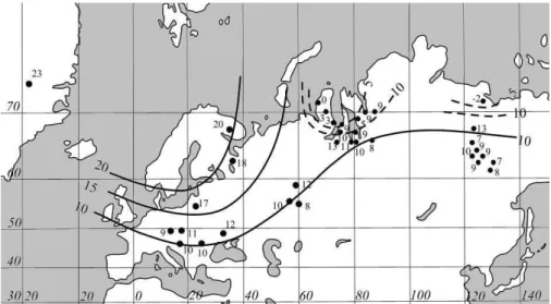
Fig. 1. Locations of the geothermal estimates of Pleistocene-Holocene warming (PHW)

ampli-tude. Numbers next to the estimates are the same as in Table 1.

(22)

CPD

3, 607–630, 2007

Full Screen / Esc

EGU

Fig 2. The spatial distribution of the geothermal estimates of PHW amplitude in Northern

Fig. 2. The spatial distribution of the geothermal estimates of PHW amplitude in Northern

Eurasia (K). Solid lines represent the main pattern the distribution follows; dashed lines show local anomalies.

(23)

CPD

3, 607–630, 2007

Full Screen / Esc

EGU

Fig. 3. Isolevel surfaces of functionalM(ϕ₀, λ₀) (left panels), and the dependence of PHW amplitude on the distance from the center of warming (right panels) for models S1–S3.

(24)

CPD

3, 607–630, 2007

Full Screen / Esc

EGU

Fig. 4. The spatial distribution of PHW amplitudes in Northern Eurasia (K) according the model

(25)

CPD

3, 607–630, 2007

Full Screen / Esc

EGU

Fig. 5. The Influence of Late Pleistocene ice sheets on the basal temperature. The solid

lines with points show the initial temperature distribution; the dashed lines show the station-ary temperature distribution with no vertical ice advection; the solid lines show the stationstation-ary temperature distribution with vertical ice advection.