HAL Id: hal-00316262
https://hal.archives-ouvertes.fr/hal-00316262
Submitted on 1 Jan 1996
HAL is a multi-disciplinary open access
archive for the deposit and dissemination of sci-entific research documents, whether they are pub-lished or not. The documents may come from teaching and research institutions in France or abroad, or from public or private research centers.
L’archive ouverte pluridisciplinaire HAL, est destinée au dépôt et à la diffusion de documents scientifiques de niveau recherche, publiés ou non, émanant des établissements d’enseignement et de recherche français ou étrangers, des laboratoires publics ou privés.
Modelling high-latitude electron densities with a
coupled thermosphere-ionosphere model
J. Schoendorf, A. D. Aylward, R. J. Moffett
To cite this version:
J. Schoendorf, A. D. Aylward, R. J. Moffett. Modelling high-latitude electron densities with a coupled thermosphere-ionosphere model. Annales Geophysicae, European Geosciences Union, 1996, 14 (12), pp.1391-1402. �hal-00316262�
Correspondence to: J. Schoendorf
Ann. Geophysicae 14, 1391—1402 (1996) ( EGS — Springer-Verlag 1996
Modelling high-latitude electron densities with a coupled
thermosphere-ionosphere model
J. Schoendorf1, A. D. Aylward1, R. J. Moffett2
1 Atmospheric Physics Laboratory, University College London, London, UK 2 Upper Atmosphere Modelling Group, University of Sheffield, Sheffield, UK Received: 15 February 1996/Revised: 23 July 1996/Accepted: 30 July 1996
Abstract. A few of the difficulties in accurately modelling high-latitude electron densities with a large-scale numer-ical model of the thermosphere and ionosphere are ad-dressed by comparing electron densities calculated with the Coupled Thermosphere-Ionosphere Model (CTIM) to EISCAT data. Two types of simulations are presented. The first set of simulations consists of four diurnally reproducible model runs for a Kp index of 4o which differ only in the placement of the energetic-particle distribution and convection pattern input at high latitudes. These simulations predict varying amounts of agreement with the EISCAT data and illustrate that for a given Kp there is no unique solution at high-latitudes. Small changes in the latitude inputs cause dramatic changes in the high-latitude modelled densities. The second type of simulation consists of inputting statistical convection and particle precipitation patterns which shrink or grow as a function of Kp throughout a 3-day period 21—23 February 1990. Comparisons with the EISCAT data for the 3 days indi-cate that equatorward of the particle precipitation the model accurately simulates the data, while in the auroral zone there is more variability in the data than the model. Changing the high-latitude forcing as a function of Kp allows the CTIM to model the average behavior of the electron densities; however at auroral latitudes model spatial and temporal scales are too large to simulate the detailed variation seen in individual nights of data.
1 Introduction
The processes governing the physics and chemistry of the upper atmosphere can be simulated using numerical modelling techniques. Large numerical thermosphere-ionosphere models such as the Coupled Thermosphere-Ionosphere Model (CTIM) (Fuller-Rowell et al., 1987) and the NCAR-TIGCM (Roble et al., 1988), have been used
extensively to study the thermospheric response to solar radiation and magnetospheric and ionospheric coupling. The results obtained from these models can be compared to data, and in turn the models are refined in light of the comparisons. As data from new satellites and ever-im-proving ground-based techniques like incoherent-scatter radar give higher-resolution measurements, the numerical models must improve in line with the data.
Numerical models of the thermosphere and ionosphere have been used in a number of studies to determine the basic structure, climatology, and phenomenology of the thermosphere (e.g., Fuller-Rowell et al., 1994; Millward
et al., 1993; Forbes and Roble, 1990; Maeda et al., 1989;
Roble et al., 1982, 1987). Comparisons between the coupled thermosphere-ionosphere models and data have largely been for neutral parameters and mid-latitude loca-tions (e.g., Fuller-Rowell et al., 1991; Crowley et al., 1989; Forbes et al., 1987). Direct comparisons between iono-spheric data and calculated ionoiono-spheric parameters from a global numerical model have been rare. Emery et al. (in press) compared NmF2 and hmF2 from combination AMIE and NCAR-TIGCM simulations with ionosonde measurements at various sites, and Codrescu et al. (1992) compared ionosonde measurements with foF2 and hmF2 calculated with the NCAR-TIGCM at mid-latitudes. Quegan et al. (1988) used a model of the ionosphere alone to simulate one particular experiment’s measurement of electron density in the F region, with mixed success.
Difficulties in modelling the high-latitude ionosphere with the CTIM arise from the model grid size being larger than the spatial variations of high-latitude phenomena, as well as the inaccuracy of high-latitude inputs into the model. At high latitudes, forcing by the convection pattern and heating from energetic particles drive the ionosphere. The forcing is extremely variable on short time-scales and small spatial scales, and the resulting temporal and spatial variation of the ionosphere is difficult to simulate. While theoretically it is possible to change the high-latitude inputs into the model on time-scales of a minute, this is not practical in most cases because of the introduction of numerical instabilities and large model run times
involved. This problem would best be addressed by in-creasing model resolution at high latitudes, and will not be considered in this paper.
The second problem arises from the types of high-latitude inputs used by global numerical models to drive the ionosphere. For modelling specific campaign periods, high-latitude forcing has been calculated from large quantities of data using the AMIE technique (e.g., Lu
et al., 1995; Knipp et al., 1989, 1993; Emery et al., 1990)
and input into the TIGCM (e.g., Emery et al., in press; Crowley et al., 1989). However, this is not done on a regular basis, and modelled high-latitude ionospheric parameters have not been compared to incoherent-scatter radar data for such simulations. In general, the high-lati-tude forcing and heating used by the CTIM are derived from statistical models, which makes quantitative simula-tions of the high-latitude variability virtually impossible. This paper addresses the issue of how well the high-lati-tude ionosphere is modelled using such inputs.
Direct comparisons are made between electron densi-ties measured by the EISCAT CP-3 experiment, both averaged and from an individual experiment, with those calculated by the CTIM. These two types of comparisons illustrate the effects of changing the high-latitude inputs for a given Kp and as a function of Kp, respectively. Averaged data is compared to four different model runs for the same Kp. The high-latitude forcing for these runs is altered by changing the latitudinal extent of the particle precipitation pattern and by slightly shifting the convec-tion pattern. The object of comparing the data to these four runs is to demonstrate that for a given Kp there is no unique solution, and that for a small spatial variation in the high-latitude forcing, electron densities will vary at high latitudes. Variation in the electron densities for the four runs indicates that it is possible to tune the high-latitude inputs into the model to match the data without changing the level of magnetic activity. In addition, this variation in calculated electron densities for a given Kp implies that the measured electron densities will also vary for a given Kp.
The second set of comparisons is between an individual CP-3 experiment which ran over a period of 3 days and a time-dependent model simulation for the same days. The simulation models changes in the high-latitude inputs by simply altering the size of the statistical convection and particle precipitation patterns as a function of Kp throughout the period. These comparisons demonstrate that the CTIM can simulate the general trend of the measured electron densities by forcing the model with smoothed and averaged high-latitude inputs rather than more realistic inputs derived specifically for the particular period. Equatorward of the auroral zone the simulation is quite accurate, while in the auroral zone there is far more variability in the data than the model, so the model predicts average behavior.
2 Model and data description
The CTIM evolved from a model of the thermosphere developed at University College London (Fuller-Rowell
and Rees, 1980) and an ionospheric model developed at Sheffield University (Quegan et al., 1982). The ionosphere and thermosphere are coupled through energy and mo-mentum interchange, so joining these models made obvi-ous sense. At first this was done on an ad hoc basis by exchanging outputs and using these as constraints on independent runs of the models (Fuller-Rowell et al., 1984), but by the mid-80s they had been coupled math-ematically into one program (Fuller-Rowell et al., 1987). The ionosphere code models the polar and auroral regions where the field lines are ‘‘open’’ and follow the high-latitude convection pattern caused by coupling be-tween the interplanetary magnetic field (IMF) and the Earth’s magnetosphere. It was found that this ‘‘open’’ region could actually be extended to a fairly low latitude (30°—50°) where the (closed) plasma tubes had such large volumes they never filled and so acted very like open plasma tubes. An empirical model (Chiu, 1975) is used for the low-latitude ionosphere (30°N—30°S).
The coupling between the ionospheric and thermo-spheric codes is complicated by the fact that they use different coordinate systems. Thermospheric parameters are calculated in the Eulerian frame (fixed to the Earth) on a grid consisting of 20 equally spaced longitude bins (every 18°), 91 bins of 2° latitude, and 15 constant-pressure level surfaces at one-scale-height separations from a lower boundary at 80 km (1 Pa). It is more convenient to calcu-late ionospheric parameters in a Lagrangian system, and in order to couple the ionospheric model to the thermo-spheric model, a semi-Lagrangian frame was implemented (Fuller-Rowell et al., 1987). Interpolation routines are used at the end of the ionospheric calculation cycles to transpose the ion results onto the thermospheric grid. The thermospheric code solves the three-dimensional energy, momentum, and continuity equations for the three major neutral species O, N2, and O2, with dependent calcu-lations of the minor neutral species. The ionospheric code solves the continuity, energy, and momentum equations for the major ion species which are constrained to the flux tubes of the Earth’s magnetic field.
The coupled model first calculates ionospheric para-meters because of the global importance of the energy and momentum inputs into the thermosphere via the high-latitude ionosphere. Locally these inputs can be equiva-lent to or greater than solar insolation. Transport of the energy and momentum gives measurable effects to low latitudes, well away from the source regions. The mo-mentum input comes mainly from the plasma flows pro-duced by the electric field inpro-duced across the Earth’s magnetic polar region by the interaction of the Earth’s magnetic field and the solar wind with its embedded IMF. Merging of the IMF and the Earth’s field (Dungey, 1961) and a possible viscous interaction at the flanks of the magnetosphere (Axford and Hines, 1961) cause plasma-flow cells to be set up in the magnetosphere. These are mapped down into the high-latitude ionosphere and are thought to take the form of a double-cell circulation pattern (e.g., Heppner and Maynard, 1987; Heelis et al., 1982) particularly when Bz (the north-south component of the IMF) is southwards. The CTIM uses a convection model such as Rich and Maynard (1989) for calculating
Fig. 1a–c. Rich and Maynard (1989) statistical convection patterns for Kp"4o on a magnetic latitude vs. MLT grid. a Default pattern used in RUN-DEF and RUN-1; the cross-cap potential drop is 82 kV. b RUN-2 convection pattern shifted slightly towards the day; the cross-cap potential drop is 65 kV. c RUN-3 convection pattern shifted slightly towards the morning; the cross-cap potential drop is 65 kV. The diamonds and circles represent the position of 68°N, 18°E and 72°N, 18°E geographic, respectively, in corrected geomagnetic coordinates. The perimeter latitude is 50°N magnetic
the momentum inputs and Joule heating due to the elec-tric fields.
Associated with these circulation patterns are regions of particle precipitation, as seen from the ground in their most energetic form as the aurorae. The pattern of precipi-tation is complex, with a number of different regions (Kamide and Akasofu, 1975). Over the polar cap there is a steady ‘‘drizzle’’ of low-energy particles, but the most energetic input occurs at or near the boundary between open and closed field lines where the ‘‘auroral oval’’ has been described from ground-based and satellite observa-tions. Empirical models of the precipitation in the auroral oval are derived from averages of large numbers of satel-lite overpasses (e.g., Fuller-Rowell and Evans, 1987; Hardy et al., 1985). The passes are binned by Kp and particle energy level, so the patterns tend to be spread geographically over a far larger area than any one indi-vidual precipitation event seen by the satellites. Energetic particle distributions such as that calculated by Hardy
et al. (1985) are input into the CTIM.
EISCAT, the European Incoherent Scatter radar asso-ciation (Rishbeth and Williams, 1985), started operations in autumn 1981, and there have been continual improve-ments in the system since then. It is capable of measuring a range of E- and F-region parameters to a time resolution of seconds or less, and to spatial resolutions of a few kilometers down to a few hundred meters, depending on conditions and experimental set-up. The CP-3 data is measured with the EISCAT UHF (933-MHz) radar, which is a tristatic system with a transmitter and receiver in Tromsø, Norway (70°N, 19°E Geographic, and 68°N, 104°E Magnetic), and receivers in Kiruna, Sweden and Sodankyla¨, Finland. These enable full tristatic velocities to be obtained for the intersection volume, while at the same time a range profile of the scalar parameters to be obtained at Tromsø.
The EISCAT CP-3 experiment includes a 16-position latitudinal scan perpendicular to the L-shells. At F-region altitudes the scan covers longitudes from about 19° to 25°E and latitudes from 65° to 74°N. Since the CTIM grid points are widely spaced, every 2° in latitude and 18° in longitude, EISCAT electron densities are binned every 2° in latitude and the longitudinal variation is ignored for this comparison.
Two years of winter CP-3 data near solar maximum were chosen at random from the EISCAT analyzed para-meter database. The data consist of 6 days: 31 January—8 March 1989, and 3 days: 21—23 February 1990. The Kp for this period varies from 0#to 6o with an average value of 4!.
Four comparisons are made between averaged EIS-CAT data and the CTIM at 140- and 300-km altitudes. The data are averaged hourly and are compared to output from diurnally reproducible simulations for February conditions modelled with an F10.7-cm flux of 185 and a Kp value of 4o. The simulations differ only in the high-latitude energetic-particle precipitation distribution and the placement of the convection pattern. Two runs, labelled RUN-DEF and RUN-1, are forced with the Rich and Maynard (1989) convection pattern illustrated in Fig. 1a. The circles and diamonds represent the
geographic locations of 72°N, 18°E and 68°N, 18°E, re-spectively, in corrected geomagnetic coordinates through-out the day. Data and model comparisons are made at these locations, and the positions of the circles and dia-monds with respect to the convection pattern will be discussed in detail in a later section. RUN-2 and RUN-3 are forced with similar convection patterns, however the patterns are slightly shifted towards the dayside (Fig. 1b) and the morningside (Fig. 1c), respectively.
Fig. 2a, b. Energetic-particle precipitation patterns for Kp"4o on a magnetic latitude vs. MLT grid. a Particle precipitation distribu-tion of Hardy et al. (1985); b new particle precipitadistribu-tion distribudistribu-tion derived from Hardy et al. (1985). The perimeter latitude is 50°N magnetic
The statistical particle precipitation pattern (Hardy
et al., 1985) used by RUN-DEF is illustrated in Fig. 2a. In
general, any single auroral oval would not be as wide as this distribution. Therefore, a new energetic-particle pat-tern has been calculated from this distribution by isolating the bins containing the maximum energy at each longi-tude and placing these bins along the convection reversal boundary. At each longitude, half the energy from the bin on either side of the convection reversal boundary is dumped into the bin along the boundary. Moving latitudi-nally outwards (poleward and equatorward) from the con-vection reversal boundary, half the energy from each bin is dumped into its neighbor’s bin nearer the boundary. The latitudinal spread of the distribution is thus decreased, but the same total energy is maintained (Fig. 2b).
While the new particle precipitation pattern is no more realistic than the default pattern, it is adequate to illus-trate that small variations in the placement of this high-latitude input result in a varied response from the ionosphere. This new energetic-particle distribution is placed along the convection reversal boundaries of the patterns shown in Fig. 1 for simulations RUN-1, RUN-2, and RUN-3, respectively. Differences in the electron dens-ities calculated in these runs are examined and compared to the averaged data.
Simulations illustrating the effect of varying the model forcing as a function of Kp are generated by using the 3-h
Kp indices and daily F10.7-cm fluxes for 21—23 February
1990 as inputs. The high-latitude forcing consists of pat-terns such as the default Rich and Maynard (1989) pattern and Hardy et al. (1985) particle precipitation pattern de-picted in Figs. 1a and 2a, respectively. Direct comparisons are made between these model runs and the 3 days of data. For the diurnally reproducible simulations the model is left to iterate to a steady state. The input parameters are fixed and the model runs through several simulated 24-h periods until the day-to-day variations stabilize. Under time-varying conditions, however, the model is initiated from a steady-state simulation similar to conditions at the beginning of 20 February 1990. It is run for the following 4 days, changing the high-latitude inputs every 3 h as a function of Kp. Previous simulations with the CTIM and NCAR-TIGCM modelling time-dependent forcing have compared well with data (e.g., Forbes et al., 1987).
3 Modelled and measured electron densities at 140 km Electron densities predicted by the four diurnally repro-ducible CTIM simulations are compared to EISCAT CP-3 densities averaged hourly over the 9 days near February solar maximum at 140 km. Although the runs are all for the same Kp, the agreement between each simulation and the data differs depending on the location of the high-latitude forcing for each simulation.
Dayside electron densities at latitudes from 66°—74° and 140 km are primarily due to photoionization. On the nightside, electron densities which are as large or larger than daytime densities are expected if auroral particle precipitation occurs at these latitudes. As an example of where the default model run (RUN-DEF) places EISCAT with respect to the high-latitude electron densities, Fig. 3 presents polar plots of electron densities calculated by the model at 140 km for 0, 6, 12, and 18 UT. The densities are plotted on geographic latitude vs. local time polar dials with the north pole in the center and 50°N latitude at the perimeter. Local noon is at the top. At each UT, the locations of 68° and 72° latitudes and 18° longitude (near EISCAT) are marked with a circle. For example, at 0 UT, EISCAT is in the midnight sector and is in the peak of the modelled electron densities. At 6 UT, EISCAT is located towards the edge of the high-density region, and at 12 UT it is on the dayside. At 18 UT, EISCAT is in the evening sector, and is again near the modelled high-density region. Using Fig. 3 as a guideline, it is expected that EISCAT will measure enhanced electron densities both pre- and post-midnight (Fig. 3a, d) until approximately 6 UT.
Modelled electron densities at 140 km are compared to the averaged CP-3 densities at 68° and 72°N as a function of UT (Fig. 4). The asterisks represent the hourly averaged data at the given latitude and the three lines represent the simulated electron densities at the same latitude as the data as well as latitudes which are 2° on either side of it. The variation in the modelled density as a function of latitude can be significant at high latitudes, particularly near regions of enhanced particle precipitation. For
Fig. 3a–d. Modelled Ne (RUN-DEF) at 140 km and a 0 UT (Ne ranges from 1.24]108 to 1.69]1011 m~3), b 6 UT (Ne ranges from 1.37]108 to 1.75]1011 m~3), c 12 UT (Ne ranges from 1.27]108 to 1.74]1011 m~3), d 18 UT (Ne ranges from 1.23]108 to
1.72]1011 m~3). The perimeter latitude is 50°N geographic, and local noon is at the top
Fig. 4a, b. RUN-DEF Ne (lines) and measured Ne (asterisks) at 140 km and 18°E. a data at 68°, b data at 72°. The dotted line is at the latitude of the data minus 2°, dashed line is at the same latitude as the data, and the dot-dash
line is at the latitude of the data plus 2°
example, modelled electron densities at 66°, 68°, and 70° are presented in Fig. 4a. During the nighttime hours, the electron density at 66° (dotted line) is considerably smaller than that at 68° (dashed line), since EISCAT’s longitude 66° is at the equatorward edge of the particle precipitation (i.e., Fig. 3a, d). However, the densities at 70° (dot-dash) are larger than those at 68°, since 70° is more often nearer the peak of the distribution. For example, at 18 UT, the model calculates densities of 5]1010 m~3 at 66°, while at 70° the densities are approximately doubled, near 1.1]1011 m~3. On the other hand, during the day (i.e., Fig. 3b, c), electron densities at the three latitudes are all very much the same, since the particle precipitation is offset towards the nightside and the three representative
latitudes in each plot are equatorward of the precipitating particles.
Measured and modelled electron densities at 140 km and 68° agree very well from 6 to 16 UT. While EISCAT is on the dayside, there is a small maximum in measured and modelled electron densities due to photoionization (Fig. 4a). However, the model overestimates the nightside electron densities at the three representative latitudes. At 72° (Fig. 4b), the model and data agree from about 0 until 14 UT but the model overestimates the measured densities in the evening sector. Modelled densities are overes-timated on the nightside at 68° and in the evening at 72° because the input particle precipitation pattern (Fig. 2a) is spread out over a wide latitude range. Therefore, EISCAT
Fig. 6a, b. Same as Fig. 4 but for RUN-1 Fig. 5a–d. Modelled Ne (RUN-1) at 140 km and a 0 UT (Ne ranges from 1.24]108 to
1.70]1011 m~3), b 6 UT (Ne ranges from 1.35]108 to 1.75]1011 m~3), c 12 UT (Ne ranges from 1.28]108 to 1.73]1011 m~3), d 18 UT (Ne ranges from 1.24]108 to
1.71]1011 m~3). The perimeter latitude is 50°N geographic, and local noon is at the top
is always in the modelled auroral zone on the nightside (e.g., Fig. 3d). Since the 68° nighttime modelled densities are larger than the CP-3 densities, and because 68° lati-tude is inside the modelled auroral oval at night (Fig. 3), it can be inferred that in this data the electron-density en-hancements at EISCAT due to nighttime auroral activity do not reach 68°. At 72°, the data match the modelled values in the morning, but are smaller than the model in the evening, implying that auroral enhancements in the data are apparent in the morning sector but not the evening sector. Therefore, EISCAT should be located equatorward of most of the auroral particle precipitation in the evening sector, even at 72° latitude.
High-latitude electron densities at 140 km calculated using the new particle precipitation distribution of Fig. 2b (RUN-1) are constrained to a narrower area (Fig. 5). Therefore, RUN-1 places EISCAT in a different position with respect to the auroral oval than does RUN-DEF. For example, at 0 UT, EISCAT is on the equatorward edge of the aurorally driven electron densities, while for RUN-DEF (Fig. 3a) it is in the peak of the density distribution. At 6 UT, EISCAT is located outside the auroral zone altogether. At 12 UT, it is on the dayside, and at 18 UT it is in the auroral zone, but near the equatorward edge.
RUN-1 electron densities are presented along with the averaged EISCAT data at 140 km in Fig. 6. At 68° the
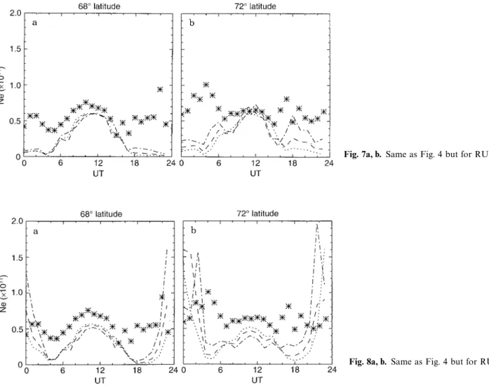
Fig. 8a, b. Same as Fig. 4 but for RUN-3 Fig. 7a, b. Same as Fig. 4 but for RUN-2
electron densities from 0—6 UT are much smaller than the RUN-DEF densities (Fig. 4) and underestimate the data. The modelled densities at 66°, 68°, and 70° are similar, since these latitudes are outside the RUN-1 auroral oval. On the dayside the densities are similar to the RUN-DEF and EISCAT densities. In the evening sector, the 66° and 68° lines approximate the densities fairly well, but the 70° line greatly overestimates the RUN-DEF and EISCAT densities. Because the energetic particles were con-solidated into fewer latitude bins, the latitudinal gradients of the distribution are larger, and the evening-sector modelled densities are far more variable than their RUN-DEF counterparts, which are calculated using a wider distribution of energies.
At 72° (Fig. 6b), the model greatly underestimates the densities in the morning and greatly overestimates them in the evening. With the high-latitude forcing in the RUN-1 configuration, the modelled electron densities are ex-tremely variable as a function of latitude. For example, at 70° (dotted line) the densities have a large peak near 20 UT, at 72° (dashed line) it occurs near 18 UT, and at 74° it peaks near 16 UT. With the high-latitude inputs in this configuration, the model predicts that EISCAT is in the auroral zone in the evening sector, but is equatorward of it postmidnight. The difference between the RUN-DEF
and RUN-1 densities on the nightside illustrates the deli-cacy involved in correctly specifying the high-latitude forcing.
Electron densities modelled with the convection and Fig. 2b particle precipitation patterns shifted slightly to-wards the dayside (RUN-2) are compared to data in Fig. 7. In this simulation there are no enhanced electron densities on the nightside from 66°—70°. At 72° (Fig. 7b) there is a slight evening-sector enhancement, but the dens-ities are still small. While the dayside measured and modelled densities are similar, nightside modelled densit-ies are too low. In the evening sector, RUN-2 places EISCAT equatorward of the auroral particle precipita-tion, while RUN-1 and RUN-DEF place EISCAT some-where in the auroral zone. In the morning sector, RUN-2 is similar to RUN-1, and places EISCAT equatorward of the energetic particles.
Figure 8 presents the electron densities from RUN-3, which were modelled by shifting the particle precipitation and convection slightly to the morningside. At 68°, modelled electron densities follow the general trend of the measured densities from 2 to 15 UT. However, in general the modelled values are too small. At both 68° and 72° modelled densities are far too large near midnight. Be-cause the high-latitude forcing is shifted towards morning,
Fig. 9a–d. Measured (asterisks) and modelled (lines) electron densities at 300 km and 72°N. a RUN-DEF, b RUN-1, c RUN-2, and d RUN-3. The dotted line is at the latitude of the data minus 2°, dashed line is at the same latitude as the data, and the dot-dash line is at the latitude of the data plus 2°
RUN-3 places EISCAT in the peak of the energetic par-ticles at these times. At most other times the RUN-3 location of EISCAT is equatorward of the precipitating particles.
Comparisons of electron densities from the four model runs illustrate that for small variations in the specification of the high-latitude inputs for a given Kp, the modelled densities vary significantly at high latitudes, particularly at night. In addition, comparisons of these model runs with EISCAT data imply that a configuration of high-latitude inputs can be found such that model electron densities will agree with EISCAT data at all UTs.
4 Electron densities at 300 km
Near EISCAT, the F-region response to the high-latitude inputs is complex because electron densities are greatly influenced by plasma flows in addition to the in situ forcing from the soft particle precipitation. EISCAT can be considered either a high- or mid-latitude site depending on its position with respect to the cusp region and the convection pattern. On the dayside, the cusp is usually to the north of EISCAT and the ion circulation is either north of EISCAT or over EISCAT, depending on condi-tions. Diurnal variations in electron density therefore are either influenced by transport or follow the availability of F-region solar insolation, with a sharp dawn rise at the onset of photoionization and a fairly rapid fall-off at dusk (Lockwood et al., 1984).
Because of EISCAT’s location near the convection-driven plasma flows, the nightside F region is rarely as empty as the purely insolation-controlled case implies. Additional sources of plasma in the EISCAT beam in-clude plasma carried along either by electrodynamic for-ces or by the neutral wind. Plasma can be carried from the dayside to the nightside in the main antisunward flow across the polar cap. Other nightside sources include local precipitation regions.
In this section, diurnal variations of hourly averaged CP-3 data at 300 km are compared to modelled electron densities at 72° (Fig. 9) and 68° (Fig. 10). Diurnal vari-ations in the EISCAT data at 72° and 68° differ because at 72° the EISCAT beam is pointed northward, toward the convection-driven plasma flows, and at 68° the beam points southward away from the high-latitude forcing. The 72° densities are not constant at night, and increase to a sharp narrow peak during the day (e.g., Fig. 9a), illustrat-ing the effects caused by the plasma flow sweepillustrat-ing densit-ies from one region and depositing them elsewhere. At 68° (e.g., Fig. 10a), densities illustrate typical solar-insolation-driven behavior of a low value at night, and a sharp rise to a broad peak in the daylight hours.
Modelled and measured electron densities at 72° are compared in Fig. 9. RUN-DEF, RUN-1, and RUN-2 model the general trends seen in the data, although RUN-DEF underestimates the peak near 10 UT and RUN-2 overestimates the postmidnight densities. The increase in RUN-1 dayside densities over RUN-DEF den-sities is due to the rebinning of the energetic particles into
Fig. 10a, b. Measured (asterisks) and modelled (lines) electron densities at 300 km and 68°N. a RUN-1, and b RUN-3. The lines are the same as Fig. 9
the configuration of Fig. 2b. In the new configuration, the dayside soft particle precipitation maximizes about 2° (one grid point) lower in latitude with almost 2.5 times the maximum energy than the default distribution. There-fore, although the RUN-1 and RUN-DEF convection patterns are colocated, the RUN-1 dayside precipitation is stronger and closer to EISCAT. RUN-2 densities differ from those of RUN-DEF and RUN-1 because RUN-2 has a dayside shift of the convection pattern and energetic particles.
The diurnal variation of RUN-3 electron densities (Fig. 9d) differs from the others because of the shift in the RUN-3 high-latitude inputs towards the morning. On the dayside, the particle precipitation and convection pattern are shifted towards higher latitudes, placing EISCAT at mid-latitudes with respect to the high-latitude forcing. At 72°, the RUN-3 diurnal variation is unlike the data and the other model runs because it demonstrates the insola-tion-driven sharp rise from a minimum near dawn and fast decrease to another minimum near dusk with a broad peak in between.
Modelled and measured densities at 68° are compared for RUN-1 and RUN-3 in Fig. 10. The measured dayside density peak is broader at 68° than 72°, and resembles a mid-latitude peak rather than a sharper high-latitude peak which is influenced by transport and energetic par-ticles. RUN-1 agrees well with the data, underestimating the densities only from 7 to 10 UT. At 68°, RUN-3 agrees well with the data from 3 to 23 UT, and is the only run to model the solar-insolation-driven behavior of a broad dayside peak and the slope of the data on either side.
Comparisons of electron densities from the four model runs illustrate a varied F-region response to the high-latitude forcing which depends on EISCAT’s location with respect to the soft particle precipitation and convec-tion-driven plasma flows. Solar insolation is the same in all four runs, so in the absence of the high-latitude forcing and heating, electron densities in all runs should be similar to those of RUN-3 on the dayside (Figs. 9d and 10b). The F-region electron densities differ among the runs largely because shifting the convection pattern causes EISCAT to be in a different place with respect to the plasma flows. For example, the locations of the circles (72°N, 18°E
Geographic) and diamonds (68°N, 18°E Geographic) with respect to the convection pattern in Fig. 1a illustrate that for RUN-DEF and RUN-1, EISCAT is expected to be in the high-latitude circulation at most times. The 68° loca-tion is equatorward of the convecloca-tion for more daylight hours than the 72° location, so fewer transport effects are apparent on the dayside. Both modelled and measured densities indicate this is the case: the higher-latitude RUN-1 and EISCAT densities (Fig. 9b) do not resemble densities affected by insolation only as closely as those at 68° (Fig. 10).
Shifting the convection pattern slightly towards the dayside (Fig. 1b) causes EISCAT to be in the high-latitude circulation except for in the evening. This is apparent in the extremely small premidnight RUN-2 densities in Fig. 9c. The morningside shift of the convection pattern (Fig. 1c) causes EISCAT to be outside the plasma flows entirely on the dayside, so that RUN-3 shows only insola-tion-driven behavior on the dayside at both latitudes. This shift also causes EISCAT to pass through the center of the dawn convection cell, causing the unreasonably large densities apparent at night.
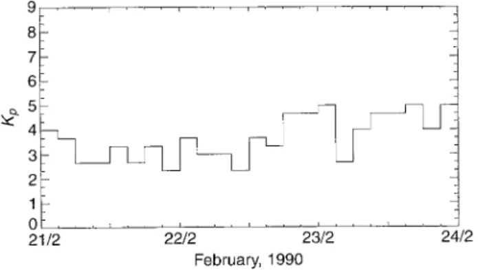
5 Individual days of data vs. time-dependent simulations In addition to modelling diurnally reproducible condi-tions by forcing the model with one convection pattern, the CTIM simulates time-dependent conditions by chang-ing the high-latitude inputs as a function of Kp. The time-dependent simulations calculate the statistical pat-terns of Rich and Maynard (1989) and Hardy et al. (1985) as a function of Kp for the period 21—23 February 1990. The Kp index for the February 1990 data varies from 2# to 5o with an average value of 4! (Fig. 11).
Comparisons between modelled and measured densi-ties at 300 km (Fig. 12) are presented at 64° (equatorward of the high-latitude forcing) and at 72° (in the high-lati-tude forcing). Equatorward of the high-latihigh-lati-tude forcing (Fig. 12a) there is little scatter in the data as a function of UT. Modelled electron densities vary little as a function of latitude because 62°—66°N are away from the region of high-latitude heating and forcing. The maxima, minima,
Fig. 13a, b. Modelled (lines) and measured (asterisks) Ne at 140 km for 21—23 February 1990. a 68°, b 72°. The lines are the same as Fig. 9
Fig. 12a, b. Modelled (lines) and measured (asterisks) Ne at 300 km for 21—23 February 1990. a 68°, b 72°. The lines are the same as Fig. 9
Fig. 11. Kp indices for 21—23 February 1990
and slope of the measured electron densities are matched by the model, except near 6 UT, where the model predicts a local maximum (similar to the one seen in Fig. 9), and on the first day when model values are smaller than the daytime densities. It is not clear why this peak is not simulated as well as the subsequent two peaks, since the model was run for the previous day as well, setting up the proper conditions for this period.
Where the EISCAT beam is pointed northward into the plasma flows at 72° (Fig. 1a), there is more variability
in the data, particularly at night (Fig. 12b). Modelled values are variable as a function of latitude, and are similar to the measured values. The change in density from night to day is well modelled.
Model predictions of electron densities at 140 km are compared to the EISCAT data for this period in Fig. 13. At 140 km and 68° the model captures the day-to-day variations seen in the data. At 72°, the data is variable enough so that it is difficult to pick out a specific trend; however the overall value of modelled electron densities matches that of the data.
Electron densities predicted by the CTIM forced with statistical high-latitude inputs are consistent with those measured by EISCAT, particularly equatorward of the energetic particles and convection pattern. In the auroral zone at 140 km and within the high-latitude circulation at 300 km there is so much variability in the data that with the existing high-latitude inputs the model is capable of only predicting overall values.
6 Conclusions
Models such as the CTIM are usually forced with statist-ical convection and energetic-particle precipitation pat-terns at high latitudes. It is generally accepted that these
patterns lead to realistic global energy input into the thermosphere, and so are adequate inputs for modelling latitudes equatorward of the high-latitude circulation. However, the modelled ionosphere in the vicinity of the inputs has not been examined in any detail in the past.
Therefore, the effectiveness of specifying statistical forc-ing for modellforc-ing the high-latitude ionosphere is exam-ined. CTIM electron densities are compared to electron densities measured by EISCAT at 140 and 300 km as a function of UT. The simulations have been divided into two sets. The four model runs from the first set of simula-tions are all for the same level of magnetic activity, and differ only in the placement of the input high-latitude convection and energetic-particle patterns. Default high-latitude forcing consists of statistical convection and ener-getic-particle precipitation patterns for a Kp index of 4o. The energetic-particle distribution is altered by narrowing the latitudinal extent of the particle precipitation pattern from about 15° to about 7° at its widest point and placing it along the convection reversal boundary. The three addi-tional model runs are forced with the new particle distri-bution and the default convection pattern; however these are input in slightly different locations in each case. One run leaves them centered on the magnetic pole, and the other two runs shift the inputs slightly towards the day-side and towards the morningday-side, respectively.
The purpose of the first set of four simulations is to use the EISCAT densities as a reference for examining the differences among the four model runs. For example, measured densities at 140 km are used as a reference for determining where the nightside hard particle precipita-tion might be expected. Similarly, the 300-km data are used as guidelines for determining whether solar insola-tion, plasma flows, or soft particle precipitation are predominantly influencing the densities in each case. In addition, the data are a guide for determining whether variations in modelled densities as a function of UT are reasonable, and whether the magnitudes of modelled densities are close to the expected values.
Comparisons of electron densities from the four model runs illustrate that for small variations in the high-latitude forcing, the modelled electron density varies significantly at high latitudes. For example, at 140 km, the densities differ mainly at night because they are predominantly affected by the in situ hard particle precipitation which is located in different positions in each case. At 300 km, the runs differ at all UTs because in addition to the influence of the soft particle precipitation on the dayside, densities are affected by transport processes due to the convection-driven plasma flows.
Comparisons of modelled electron densities with EIS-CAT data demonstrate differing agreement between the data and each run. The CTIM does not predict the entire UT variation of the electron densities in any one run. However, it predicts part of it in some of the runs. This indicates that any one of the set of high-latitude inputs, particularly the energetic-particle precipitation pattern, is not in the right place with respect to EISCAT at all UTs. Changing the high-latitude forcing a little bit produces large enough changes in the modelled electron densities so agreement with the data also changes.
However, while it might be possible to gain better agreement with data, care must be taken to be sure that the correct mechanism is causing the agreement. For example, EISCAT is generally considered to be too far equatorward of the F-region dayside soft particle precipi-tation to be affected by it. However, modelled dayside densities at 300 km are influenced by the particle precipi-tation. The increase in RUN-1 dayside densities over RUN-DEF densities indicates that shifting the soft par-ticle precipitation 2° equatorward is enough to cause increases in the modelled dayside densities at EISCAT. RUN-DEF and RUN-1 share the same convection pat-tern, so differing transport effects will be minimal.
If in reality the cusp region is north of EISCAT, then in the F-region RUN-DEF dayside densities should agree better with the data than the RUN-1 densities. Also, the added effects of the particle precipitation should cause 1 to overestimate the data. However, it is the RUN-1 densities that agree with the maximum value of the dayside densities. Therefore, while changing the high-latitude inputs gives better agreement with the data, it is not clear that it is the correct mechanism that is causing the improvement.
In the auroral zone at 140 km, densities at EISCAT are predominantly influenced by the in situ hard particle precipitation at night, so placement of the energetic-par-ticle distribution is important. In general, EISCAT is not typically located in the auroral zone throughout the night. However, RUN-DEF placed EISCAT in the auroral zone at all nightside UTs. The modelled auroral oval is there-fore too large. The narrower oval used for 1, RUN-2, and RUN-3 is smaller than the default Hardy et al. (1985) oval, and although it gives an indication of what sort of densities result from more precise placement of the energetic particles, this oval does not place the energy in the right place in any of its positions.
The second set of simulations consists of model runs which vary the default statistical high-latitude forcing as a function of Kp throughout a 3-day period 21—23 Febru-ary 1990. The purpose of modelling these 3 days is to illustrate that with a typical run modelling time-varying conditions, the CTIM accurately models the electron densities equatorward of the high-latitude inputs. Compari-sons with EISCAT data for the same period demonstrate that with the default statistical high-latitude forcing, the CTIM is adequate for determining the general behavior of the high-latitude ionosphere for the given conditions.
Presenting modelled electron densities at three adja-cent latitudes in both sets of simulations demonstrates that within the region of high-latitude forcing, modelled values are extremely variable as a function of latitude. Because of the model’s large grid size and the inaccurate high-latitude forcing, it is possible that electron densities calculated by the model at a given latitude are actually simulating behavior expected at a different latitude. This is not a problem equatorward of the high-latitude inputs as there is much less variability in the modelled values as a function of latitude.
While the simulations with time-dependent forcing give the promising result of fairly accurately modelling a par-ticular period with statistical high-latitude inputs which
are not specific to that period, the first set of simulations demonstrate an inherent difficulty in accurately modelling the high-latitude ionosphere using the CTIM. For a specific
Kp, small variations in the input high-latitude forcing will
result in differing electron densities at high latitudes. There-fore, for a given Kp there is no unique solution, and a set of high-latitude inputs can be chosen to give a desired result. One of the implications of this result is its effect on the high-latitude thermosphere. Since energy and momentum are input into the thermosphere via the high-latitude ionosphere, for a given Kp there will be no one thermo-spheric solution if there is no unique ionothermo-spheric solution. The thermospheric response to the four diurnally reproduc-ible simulations will be addressed in a subsequent paper.
Overall, the comparisons imply that a configuration of high-latitude inputs can be found such that CTIM electron densities will agree with EISCAT data at all UTs. However, tuning model inputs so that the model agrees with data presents its own set of problems, such as deter-mining the extent and placement of the energetic particles and how to warp the convection pattern to suit specific needs. In addition, tuning model inputs so that the model agrees with data at one high-latitude site does not imply that the model will be accurately simulating electron dens-ities at other high-latitude locations.
Acknowledgements. Topical Editor D. Alcayde´ thanks C. Fesen and
B. Emery for their help in evaluating this paper.
References
Axford, W. I., and C. O. Hines, A unifying theory of high-latitude geophysical phenomena and geomagnetic storms, Can. J. Phys., 39, 1433—1464, 1961.
Chiu, Y. T., An improved phenomenological model of ionospheric density, J. Atmos. ¹err. Phys., 37, 1563—1570, 1975.
Codrescu, M. V., R. G. Roble, and J. M. Forbes, Interactive iono-sphere modeling — a comparison between TIGCM and ionosonde data, J. Geophys. Res., 97, 8591—8600, 1992. Crowley, G., B. A. Emery, R. G. Roble, H. C. Carlson, Jr., and D. J.
Knipp, Thermospheric dynamics during September 18—19, 1984, 1, Model simulations, J. Geophys. Res., 94, 16925—16944, 1989. Dungey, J. W., Interplanetary magnetic field and the auroral zones,
Phys. Rev. ¸ett., 6, 47—48, 1961.
Emery, B. A., A. D. Richmond, H. W. Kroehl, C. D. Wells, and J. M. Ruohoniemi, Electric potential patterns deduced for the SUN-DIAL period of September 23—26, 1986, Ann. Geophysicae, 8, 399—408, 1990.
Emery, B. A., G. Lu, E. P. Szuszczewicz, A. D. Richmond, R. G. Roble et al., AMIE-TIGCM comparisons with global iono-spheric and thermoiono-spheric observations during the GEM/SUN-DIAL period of March 28—29, 1992, J. Geophys. Res., in press Forbes, J. M., and R. G. Roble, Thermosphere-ionosphere coupling —
an experiment in interactive modelling, J. Geophys. Res., 95, 201—208, 1990.
Forbes, J. M., R. G. Roble, and F. A. Marcos, Thermospheric dynamics during the March 22, 1979, magnetic storm 2. Com-parisons of model predictions with observations, J. Geophys.
Res., 92, 6069—6081, 1987.
Fuller-Rowell, T. J., and D. S. Evans, Height-integrated Pedersen and Hall conductivity patterns inferred from the TIROS-NOAA satellite data, J. Geophys. Res., 92, 7606—7618, 1987.
Fuller-Rowell, T. J., and D. Rees, A three-dimensionsal time-depen-dent global model of the thermosphere, J. Atmos. Sci., 37, 2545—2567, 1980.
Fuller-Rowell, T. J., D. Rees, S. Quegan, G. J. Bailey, and R. J. Moffett, The effect of realistic conductivities on the high-latitude
neutral thermospheric circulation, Planet. Space Sci., 32, 469—480, 1984.
Fuller-Rowell, T. J., D. Rees, S. Quegan, R. J. Moffett, and G. J. Bailey, Interactions between neutral thermospheric composition and the polar ionosphere using a coupled ionosphere-thermo-sphere model, J. Geophys. Res., 92, 7744—7748, 1987.
Fuller-Rowell, T. J., D. Rees, H. F. Parrish, T. S. Virdi, and P. J. S. Williams, Lower thermosphere coupling study — comparison of observations with predictions of the University College London-Sheffield thermosphere-ionosphere model, J. Geophys. Res., 96, 1181—1202, 1991.
Fuller-Rowell, T. J., M. V. Codrescu, R. J. Moffett, and S. Quegan, Response of the thermosphere and ionosphere to geomagnetic storms, J. Geophys. Res., 99, 3893—3914, 1994.
Hardy, D. A., M. S. Gussenhoven, and E. Holeman, A statistical model of auroral electron precipitation, J. Geophys. Res., 90, 4229—4248, 1985.
Heelis, R. A., J. K. Lowell, and R. W. Spiro, A model of the high-latitude ionospheric convection pattern, J. Geophys. Res., 87, 6339—6345, 1982.
Heppner, J. P., and N. C. Maynard, Empirical high-latitude electric field models, J. Geophys. Res., 92, 4467—4489, 1987.
Kamide, Y., and S.-I. Akasofu, The auroral electrojet and global auroral features, J. Geophys. Res., 80, 3585—3602, 1975. Knipp, D. J., A. D. Richmond, G. Crowley, O. de la Beaujardiere, and
E. Friis-Christensen, Electrodynamic patterns for September 19, 1984, J. Geophys. Res., 94, 16913—16923, 1989.
Knipp, D. J., B. A. Emery, A. D. Richmond, N. U. Crooker, M. R. Hairstonet al.,Ionospheric convection response to slow, strong variations in a northward Interplanetary Magnetic Field: A case study for January 14, 1988, J. Geophys. Res., 98, 19273—19292, 1993.
Lockwood M., A. D. Farmer, H. J. Opgenoorth, and S. R. Crothers, EISCAT observations of plasma convection and the high-lati-tude winter F-region during substorm activity, J. Atmos. ¹err.
Phys., 46, 489—500, 1984.
Lu, G., L. R. Lyons, P. H. Rieff, W. F. Denig, O. de la Beaujardiere, H. W. Kroehl, P. T. Newell, F. J. Rich, H. Opgenoorth, M. A. L. Persson, Characteristics of ionospheric convection and field-alig-ned current in the dayside cusp region, J. Geophys. Res., 100, 11845—11861, 1995.
Maeda, S., T. J. Fuller-Rowell, and D. S. Evans, Zonally averaged dynamical and compositional response of the thermosphere to auroral activity during September 18—24, 1984, J. Geophys. Res., 94, 16869—16883, 1989.
Millward, G. H., R. J. Moffett, and S. Quegan, Effects of an atmo-spheric gravity wave on the midlatitude ionoatmo-spheric F-layer, J.
Geophys. Res., 98, 19173—19179, 1993.
Quegan, S., G. J. Bailey, R. J. Moffett, R. A. Heelis, T. J. Fuller-Rowell, D. Rees, and R. W. Spiro, A theoretical study of the distribution of ionization in the high-latitude ionosphere and the plasmasphere: first results on the mid-latitude trough and the light-ion trough, J. Atmos. ¹err. Phys., 44, 619—640, 1982.
Quegan, S., R. S. Gill, and M. Lockwood, Comparisons between EISCAT observations and model calculations of the high-lati-tude ionosphere, J. Atmos. ¹err. Phys., 50, 1057—1076, 1988. Rich, F. J., and N. C. Maynard, Consequences of using simple
analytical functions for the high-latitude convection electric field,
J. Geophys. Res., 94, 3687—3701, 1989.
Rishbeth, H., and P. J. S. Williams, The EISCAT ionospheric radar: the system and its early results, Q. J. R. Astron. Soc., 26, 478—512, 1985.
Roble, R. G., R. E. Dickinson, and E. C. Ridley, Global circulation and temperature structure with high-latitude plasma convection,
J. Geophys. Res., 87, 1599—1614, 1982.
Roble, R. G., E. C. Ridley, and R. E. Dickinson, On the global mean structure of the thermosphere, J. Geophys. Res., 87, 8745—8758, 1987.
Roble, R. G., E. C. Ridley, A. D. Richmond, and R. E. Dickinson, A coupled thermosphere/ionosphere general circulation model,