HAL Id: insu-01373957
https://hal-insu.archives-ouvertes.fr/insu-01373957
Submitted on 29 Sep 2016
HAL is a multi-disciplinary open access
archive for the deposit and dissemination of
sci-entific research documents, whether they are
pub-lished or not. The documents may come from
teaching and research institutions in France or
abroad, or from public or private research centers.
L’archive ouverte pluridisciplinaire HAL, est
destinée au dépôt et à la diffusion de documents
scientifiques de niveau recherche, publiés ou non,
émanant des établissements d’enseignement et de
recherche français ou étrangers, des laboratoires
publics ou privés.
Interannual variability of ammonia concentrations over
the United States: sources and implications
Luke D. Schiferl, Colette L. Heald, Martin van Damme, Lieven Clarisse,
Cathy Clerbaux, Pierre-François Coheur, John B. Nowak, J. Andrew Neuman,
Scott C. Herndon, Joseph R. Roscioli, et al.
To cite this version:
Luke D. Schiferl, Colette L. Heald, Martin van Damme, Lieven Clarisse, Cathy Clerbaux, et al..
Interannual variability of ammonia concentrations over the United States: sources and implications.
Atmospheric Chemistry and Physics, European Geosciences Union, 2016, 16 (18), pp.12305-12328.
�10.5194/acp-16-12305-2016�. �insu-01373957�
www.atmos-chem-phys.net/16/12305/2016/ doi:10.5194/acp-16-12305-2016
© Author(s) 2016. CC Attribution 3.0 License.
Interannual variability of ammonia concentrations over the United
States: sources and implications
Luke D. Schiferl1, Colette L. Heald1,2, Martin Van Damme3, Lieven Clarisse3, Cathy Clerbaux3,4,
Pierre-François Coheur3, John B. Nowak5, J. Andrew Neuman6,7, Scott C. Herndon5, Joseph R. Roscioli5, and Scott J. Eilerman6,7
1Department of Civil and Environmental Engineering, Massachusetts Institute of Technology, Cambridge, Massachusetts, USA
2Department of Earth, Atmospheric and Planetary Sciences, Massachusetts Institute of Technology, Cambridge, Massachusetts, USA
3Spectroscopie de l’atmosphère, Chimie Quantique et Photophysique, Université Libre de Bruxelles, Brussels (ULB), Belgium
4LATMOS/IPSL, UPMC Université Paris 06 Sorbonne Universités, UVSQ, CNRS, Paris, France 5Aerodyne Research, Inc., Billerica, Massachusetts, USA
6Cooperative Institute for Research in Environmental Sciences, University of Colorado Boulder, Boulder, Colorado, USA
7Chemical Sciences Division, Earth System Research Laboratory, NOAA, Boulder, Colorado, USA
Correspondence to:Luke D. Schiferl (schiferl@mit.edu)
Received: 2 April 2016 – Published in Atmos. Chem. Phys. Discuss.: 18 April 2016
Revised: 12 September 2016 – Accepted: 14 September 2016 – Published: 29 September 2016
Abstract. The variability of atmospheric ammonia (NH3), emitted largely from agricultural sources, is an important fac-tor when considering how inorganic fine particulate matter (PM2.5) concentrations and nitrogen cycling are changing over the United States. This study combines new observa-tions of ammonia concentration from the surface, aboard air-craft, and retrieved by satellite to both evaluate the simulation of ammonia in a chemical transport model (GEOS-Chem) and identify which processes control the variability of these concentrations over a 5-year period (2008–2012). We find that the model generally underrepresents the ammonia con-centration near large source regions (by 26 % at surface sites) and fails to reproduce the extent of interannual variability ob-served at the surface during the summer (JJA). Variability in the base simulation surface ammonia concentration is dom-inated by meteorology (64 %) as compared to reductions in SO2and NOxemissions imposed by regulation (32 %) over this period. Introduction of year-to-year varying ammonia emissions based on animal population, fertilizer application, and meteorologically driven volatilization does not substan-tially improve the model comparison with observed ammonia
concentrations, and these ammonia emissions changes have little effect on the simulated ammonia concentration variabil-ity compared to those caused by the variabilvariabil-ity of meteo-rology and acid-precursor emissions. There is also little ef-fect on the PM2.5 concentration due to ammonia emissions variability in the summer when gas-phase changes are fa-vored, but variability in wintertime emissions, as well as in early spring and late fall, will have a larger impact on PM2.5 formation. This work highlights the need for continued im-provement in both satellite-based and in situ ammonia mea-surements to better constrain the magnitude and impacts of spatial and temporal variability in ammonia concentrations.
1 Introduction
The modern agricultural system developed to feed an in-creasing human population relies heavily on artificially pro-duced reactive nitrogen in the form of ammonia (NH3). The intensification of agricultural practices has significantly per-turbed the global nitrogen cycle over the past century,
in-cluding increases in ammonia emissions into the atmosphere (Galloway and Cowling, 2002; Erisman et al., 2008; Sutton et al., 2008). Agricultural ammonia emissions contribute to inorganic fine particulate matter (PM2.5)formation (e.g., am-monium sulfate and amam-monium nitrate) in the atmosphere (Seinfeld and Pandis, 2006). PM2.5 has numerous negative effects on human health, including respiratory and cardio-vascular distress and an overall decrease in life expectancy (Pope et al., 2009). Agriculture has a large impact on PM2.5 throughout the world, contributing up to 40 % of premature mortality due to outdoor air pollution in parts of Europe (Lelieveld et al., 2015). In the United States (US), ammo-nia emissions from agriculture exports alone react to increase population-weighted PM2.5 concentration domestically by 0.36 µg m−3, with contributions greater than 1 µg m−3 in parts of the Midwest (Paulot and Jacob, 2014). Thus, the reg-ulation of ammonia emissions may have the potential to re-duce PM2.5 in ammonia-limited areas (Pinder et al., 2006), and in a sulfate-limited environment (sulfate = SO2−4 ), am-monia can play a more important role, leading to ammonium nitrate formation. However, this potential for ammonia emis-sions reductions to reduce PM2.5may be decreasing as sulfur dioxide (SO2)and NOx(nitric oxide (NO) + nitrogen diox-ide (NO2))regulation is implemented in the US (Holt et al., 2015). PM2.5also contributes to reduced environmental vis-ibility and affects the radiative budget of the earth (IPCC, 2013). Finally, the release of excess nitrogen from agricul-tural sources into the atmosphere will also increase nitrogen deposition fluxes, which can cause negative ecosystem ef-fects such as acidification and eutrophication (Erisman et al., 2007). This is of particular concern in sensitive ecosystems such as alpine terrain and wetlands (Beem et al., 2010; Ellis et al., 2013).
The magnitude and timing of the ammonia emissions from agriculture are generally less well understood than for other anthropogenic emissions (e.g., mobile sources of NOx, power plant emissions of SOx(SO2+sulfate)). A sticky gas, ammonia is difficult to measure in situ, and this can lead to a low bias in measured concentrations (von Bobrutzki et al., 2010). The paucity of observational constraints has also lim-ited the evaluation of emission inventories and the resulting PM2.5formation simulated by models. Agricultural emission inventories are often based on emission factors from animals or fertilizers under certain field conditions, which are gen-eralized to known populations or mass applied, respectively. These conditions are highly variable due to meteorology, lo-cal livestock diet, and waste management and storage (Hris-tov et al., 2011). Recent studies have established that these bottom-up inventories often underestimate ammonia emis-sions due to difficulties in effectively scaling the low-biased measurements (Walker et al., 2012). Studies in California, in particular, show evidence of this ammonia underestimate in areas with rapidly increasing livestock populations, and they encourage improvements in ammonia emissions esti-mates to better predict PM2.5 (Nowak et al., 2012; Schiferl
et al., 2014). Models that underestimate the ammonia emis-sions will underestimate the surface PM2.5if sufficient acid is available, negatively affecting air quality management. How-ever, Paulot et al. (2016) suggest that ammonium nitrate for-mation globally is more limited by nitric acid (HNO3)than ammonia, and that the uncertainty associated with the forma-tion of nitric acid via N2O5 uptake has a greater impact on ammonium nitrate formation than the uncertainty associated with ammonia emissions. Regardless, as regulations in the US restrict SO2and NOx, the proportion of reactive nitrogen deposition is shifting from oxidized to reduced forms (Pin-der et al., 2011; Lloret and Valiela, 2016), and thus the need to understand ammonia emissions and their role in the en-vironment is growing. This importance has been recognized as new observations of ammonia have become available over longer time periods and with more spatial coverage.
Given these new observations and their relevance to un-derstanding inorganic PM2.5formation, our goal is to under-stand the factors that control ammonia concentrations and their variability in the atmosphere. This study uses newly available observations to investigate the variability of ammo-nia in the US during a 5-year time period (2008–2012). We first identify observed ammonia variability and investigate the ability of a chemical transport model to reproduce these observations. Then, we attribute sources of the model am-monia concentration variability and use known relationships in an attempt to more accurately represent the variability of agricultural ammonia emissions.
2 GEOS-Chem simulation 2.1 General description
We use the GEOS-Chem chemical transport model (www. geos-chem.org) to simulate ammonia concentrations over the US. The scenarios described throughout this paper are driven by GEOS-5 assimilated meteorology for 2008 to 2012 from the NASA Global Modeling and Assimilation Office. We use v9-02 of the GEOS-Chem model in a nested con-figuration over North America at a horizontal resolution of 0.5◦×0.667◦ (Wang et al., 2004; Chen et al., 2009). The chemistry and transport time steps for these nested simula-tions are 20 and 10 min, respectively. A global simulation at 2◦×2.5◦ horizontal resolution is used to generate the boundary conditions necessary for the nested simulations. There are 47 vertical layers in all cases. The representa-tion of the sulfate–nitrate–ammonium aerosol system and its relevant precursor gases in the standard version, including emissions, chemistry, and deposition schemes, generally re-mains as that described previously in Schiferl et al. (2014). Briefly, the coupling of gas-phase chemistry to aerosol chem-istry in GEOS-Chem is described by Park et al. (2004). The gas-particle partitioning of ammonium nitrate is calculated by ISORROPIA II (Fountoukis and Nenes, 2007) as
im-plemented by Pye et al. (2009), where the aerosols are as-sumed to exist on the metastable branch of the hygroscopic hysteresis curve. Relevant modifications from v9-01-01 used in Schiferl et al. (2014) to v9-02 used here include up-dates to the seasonal cycle of the US Environmental Protec-tion Agency’s (EPA) NaProtec-tional Emissions Inventory for 2005 (NEI-2005) ammonia emissions (Zhang et al., 2012) and to the algorithm controlling soil NOxemissions (Hudman et al., 2012) (described in Sect. 2.2).
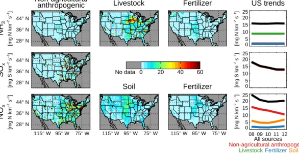
2.2 Emissions and emission trends in base scenario The “base scenario” referred to in this analysis incorporates modifications to the standard GEOS-Chem v9-02 simulation that have been made to the emissions in order to more accu-rately represent the study time period. In the base scenario, annual scale factors applied to anthropogenic SOxand NOx emissions to capture the emissions trends over time (which end in 2010 in the standard model version) are extended uni-formly spatially to 2011 and 2012 from EPA Trends data (www.epa.gov/ttn/chief/trends/). Mean anthropogenic SOx, largely from power generation, and NOx, largely from auto-mobiles, emission rates over the US in summer (JJA) 2008 are 18 mg S km−2s−1 and 16 mg N km−2s−1, respectively. As shown in Fig. 1, anthropogenic SOx and NOx emis-sions are highest in the eastern US and are often associ-ated with rural point or dense urban sources. These emis-sion rates decrease by 30 and 33 %, respectively, by 2012. The majority of the magnitude of these decreases occurs in the eastern regions of the US. For 2008, anthropogenic SOx makes up 98 % of total SOx emissions, and anthropogenic NOx makes up 65 % of total NOx emissions. Other major sources of NOx with large interannual variability are soils and fertilizer use. In the entire US, these summertime emis-sion rates vary from −23 to +20 % of the mean from 2008 to 2012, with most of the variability occurring in the Plains and the Midwest regions. The soil and fertilizer NOx emis-sion rates are simulated online and are controlled by a combi-nation of nitrogen storage and meteorology (Hudman et al., 2012). In 2012, high temperatures increase soil and fertil-izer NOxemissions, offsetting the decrease in anthropogenic NOxemissions (Fig. 1).
As in the standard version, our base scenario uses anthro-pogenic ammonia emissions from the EPA NEI-2005 inven-tory, which includes livestock, fertilizer, and non-agricultural sources. These emissions are for August and scaled uni-formly spatially each month as determined by Zhang et al. (2012). The summer mean anthropogenic ammonia emis-sion rate for the US is 12 mg N km−2s−1. Livestock and fer-tilizer use comprise 71 and 15 % of this emission rate, respec-tively. This proportion is unrealistically constant through-out the year as the scaling above does not, for example, ac-count for springtime crop fertilization. The Plains and the Midwest exhibit higher total anthropogenic emission rates of 20 and 19 mg N km−2s−1, respectively, with larger
contribu-tions from agriculture. The spatial distribution of these high ammonia emission regions are shown in Fig. 1. For the entire US, anthropogenic ammonia emissions make up 78 % of the total ammonia emissions in the summer. Other sources in-clude natural emissions (16 %), biofuel (3.7 %) and biomass burning (1.8 %). Biomass burning emissions are highly vari-able over the study period (by a factor of 2), which causes slight differences in the proportions mentioned above. In our base scenario, we use daily biomass burning emissions from the Fire INventory from NCAR (FINN) through 2012 (Wied-inmyer et al., 2011). Given a nearly constant rate of ammo-nia emission and the large changes in NOx emissions men-tioned above, changes in the ammonia concentrations may be driven by changes in the acid supply, which would affect gas-particle partitioning of ammonium nitrate and the overall PM2.5concentration.
There is no diurnal or interannual variability in the ammo-nia emissions in our base scenario. When we implement a di-urnal emission scaling determined by the local daily didi-urnal surface temperature profile, the mean surface summer am-monia concentration in the US is reduced by 12 % (1.62 ppb without vs. 1.43 ppb with diurnal emission scaling). This mean value is heavily influenced by a large daily overnight decrease in concentration of 24 %, while the daytime con-centration decrease is minimal, only 1 %. There is substan-tial uncertainty associated with any diurnal emission scaling scheme, and given its modest impact on ammonia concentra-tions (particularly in the daytime) and the minimal resulting impact on seasonal mean PM2.5 concentrations, the diurnal emission scheme is not used in this study.
We have not included any scheme that accounts for the bidirectional flux (deposition and re-emission) of ammonia in our base scenario. Rather, ammonia is permanently re-moved via wet scavenging in convective and stratiform pre-cipitation (Mari et al., 2000; Amos et al., 2012) and via sur-face resistance-driven dry deposition (Wesely, 1989). On-going research suggests that a unidirectional dry deposition scheme may be inappropriate with regards to ammonia (Mas-sad et al., 2010; Zhang et al., 2010). Under a bidirectional scheme, ammonia can be either taken up or re-emitted by a plant based on the comparison of the ambient ammonia concentration with a varying compensation point (an ambi-ent concambi-entration greater than the compensation point leads to deposition). Re-emitted ammonia has the potential to af-fect ecosystems farther downwind. Failing to account for this re-emission may locally cause an overestimation in dry de-position, resulting in low ammonia concentrations. Zhu et al. (2015) incorporate the bidirectional flux scheme of Pleim et al. (2013) into GEOS-Chem, which increases the July am-monia emissions and concentration in the US. This slightly reduces the July model bias compared to measurements at Ammonia Monitoring Network (AMoN) sites. However, the bidirectional scheme causes a decrease in ammonia emis-sions and concentration in April and October, which worsens the comparison with observations and does not account for
28° N 36° N 44° N 0 5 10 15 20 25 [mg N km − 2 s − 1] 28° N 36° N 44° N 0 5 10 15 20 25 [mg S km − 2 s − 1] 28° N 36° N 44° N 115° W 95° W 75° W 115° W 95° W 75° W 115° W 95° W 75° W 08 09 10 11 12 0 5 10 15 20 25 [mg N km − 2 s − 1] US trends All sources Non-agricultural anthropogenic LivestockFertilizerSoil
No data 0 20 40 60
Non-agricultural
anthropogenic Livestock Fertilizer
Soil Fertilizer NH 3 [mg N km − 2 s − 1] SO x [mg S km − 2 s − 1] NO x [mg N km − 2 s − 1]
Figure 1. Summer (JJA) ammonia (top row), SOx(middle row), and NOx(bottom row) emissions as implemented in the GEOS-Chem base
scenario. Maps show values for 2008; US emission rate shown for 2008 through 2012 on the right. Color bar is saturated at 60; local values may exceed this emission rate. Data outside the continental US are not shown here, nor in all subsequent figures.
missing primary emissions. Such bidirectional flux schemes, developed largely to simulate field conditions, require higher resolution observations for evaluation at finer scales than those offered by current observations and global models. 2.3 GEOS-Chem simulation of ammonia in previous
studies
A number of previous studies have evaluated the GEOS-Chem simulation of ammonia. These studies are often lim-ited in their comparison with ammonia observations and in-stead use measurements of PM2.5concentration and wet de-position flux, which are more commonly measured, to indi-rectly evaluate the model. The initial evaluation of the imple-mentation of the gas-particle partitioning mechanism by Pye et al. (2009) reveals an underprediction of inorganic aerosol in the US, but they do not attribute this bias to problems with the ammonia emissions inventory. Zhang et al. (2012) apply an updated monthly scaling to the NEI-2005 ammonia emis-sions to improve the model bias in NHx (NH3+ammonium (NH+4))based on network measurements of wet deposition fluxes over a limited timeframe. Even with these improve-ments, the model remains biased high for nitric acid, ammo-nium, and nitrate (NO−3), which they suggest is due to ex-cess production of nitric acid from N2O5hydrolysis, though Heald et al. (2012) show that altering this uptake process does not improve the simulation of nitrate in the model. An underestimate of ammonia emissions in California is sug-gested by Heald et al. (2012) and Schiferl et al. (2014) using Infrared Atmospheric Sounding Interferometer (IASI) satel-lite measurements and aircraft measurements of ammonia, respectively. Walker et al. (2012) also suggest that an
in-crease in ammonia emissions in California is required to re-duce the model bias compared to ammonium nitrate obser-vations. The GEOS-Chem adjoint is used along with Tro-pospheric Emission Spectrometer (TES) measurements by Zhu et al. (2013) to constrain ammonia emissions over the US. They find an optimized solution that increases ammo-nia emissions in Califorammo-nia and other parts of the western US and improves comparison of simulated surface concentration with observations from AMoN. Paulot et al. (2014) also use the GEOS-Chem adjoint along with ammonium wet deposi-tion measurements to similarly optimize ammonia emissions. These results increase ammonia emissions in California and the Midwest, consistent with underestimates described in previous studies, and decrease emissions in some regions of the northeast and southeast. Their optimization also suggests errors in the seasonality of emissions, particularly relating to fertilizer emissions in the Midwest.
3 Ammonia observations
3.1 IASI satellite column measurements
Recent work has shown that atmospheric ammonia concen-tration can be retrieved from satellite observations at thermal infrared wavelengths (Clarisse et al., 2009, 2010; Shephard et al., 2011; Shephard and Cady-Pereira, 2015; Warner et al., 2016). These retrievals provide greater spatial coverage of ammonia concentrations than current surface networks. Here we use a product from the IASI mission, which is designed to take full advantage of the hyperspectral character of the strument (Van Damme et al., 2014a). An infrared radiance in-dex, calculated from a wider spectral range than previous
am-monia satellite products to increase sensitivity, is converted to a total ammonia column value using look-up tables that de-pend on this index and the thermal contrast (temperature dif-ference between the surface (skin) and the air above). These look-up tables are computed using the Atmosphit forward ra-diative transfer model. The observations provide high spatial resolution (circular 12 km footprint at nadir) and up to twice-daily temporal resolution. Although there is vertical varia-tion in the concentravaria-tion sensitivity in the infrared retrieval, this information (e.g., an averaging kernel) is not available with this IASI product. However, an uncertainty estimate (re-trieval error) is associated with each individual measurement. In general, relative uncertainties are smaller for larger col-umn concentration and larger thermal contrasts. These errors range from more than 100 % to less than 25 % under good conditions. This IASI product was initially used to exam-ine both regional and global ammonia concentration varia-tion, highlighting the influence of biomass burning events on the global scale as well as the ability to capture smaller ammonia emission features (Van Damme et al., 2014a). In Van Damme et al. (2015b), seasonal patterns and interannual variability at subcontinental scale are identified and an IASI-derived climatology of the month of maximum columns is used to attribute major source processes. Ammonia column measurements from the retrieval scheme were also evalu-ated in Europe against a regional air quality model by Van Damme et al. (2014b). This comparison shows good agree-ment between observed and simulated ammonia column con-centrations in both agricultural and remote regions, although average measured columns are higher than those simulated. When accounting for the lack of retrieval sensitivity during colder months, the observations capture the seasonality sim-ulated in the agricultural regions. Van Damme et al. (2015a) attempt to validate the IASI product against in situ ammonia measurements, although this is challenging given the lack of highly spatially distributed measurements and the difference in measured quantities. The measured IASI columns tend to show less variability compared to surface measurements.
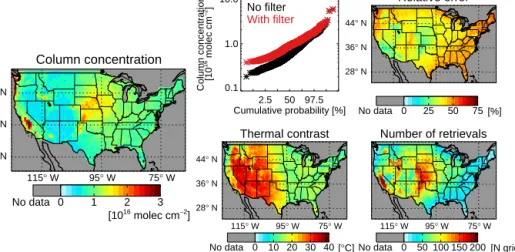
Our study uses data from the morning overpass (09:30 lo-cal solar time when crossing the Equator) of IASI onboard the MetOp-A satellite from 2008 to 2012. Each day is grid-ded by computing the mean column concentration (and other properties) weighted by relative error of the native retrievals within each GEOS-Chem horizontal grid box at the nested resolution (0.5◦×0.667◦). The results of this gridding and averaging scheme are shown in Fig. 2 as the mean of all sum-mers during the study period. We filter out retrievals with cloud cover greater than or equal to 25 % and skin tempera-ture less than or equal to −10◦C as recommended by Van Damme et al. (2014a). Post-gridded values are filtered by removing grid boxes with greater than 75 % relative error. This filtering alters the distribution of the column concen-tration by removing the smallest values, as shown in Fig. 2. We also isolate the continental US by removing grid boxes over Canada, Mexico and the ocean, but due to their size,
some grid boxes along the border may exhibit outside influ-ence (such as ocean retrievals along the Pacific Northwest coast). We calculate seasonal means as the simple arithmetic mean of all valid gridded daily values within that time pe-riod. This method weights each day with at least one valid retrieval evenly, rather than biasing the seasonal mean toward days with multiple valid retrievals in a grid box on a single day.
The gridded IASI values used in our analysis are more likely to be valid (meeting the retrieval and filtering restric-tions) on warm, cloud-free days with high ammonia concen-trations. The mean reported IASI concentrations are there-fore biased, as low ammonia concentrations are harder to de-tect with confidence, and are thus often filtered out. Most valid retrievals occur during the summer, the time of highest concentration (and emissions in most areas) and better in-frared retrieval conditions. As shown in Fig. 2, the range of mean (2008–2012) summer gridded and filtered concentra-tions is from 0.4 to 7 × 10¹⁶molec cm−2. The IASI column concentrations are highest in known agricultural regions such as the Central Valley of California, the Plains, and the Mid-west. Individual spatial features are well defined and benefit from the high horizontal resolution satellite product.
Although filtered to exclude a maximum relative error, the remaining errors remain higher along the eastern coast and throughout the southeastern US, which has lower ammonia concentrations and lower thermal contrast. The relative er-ror is also inversely related to the number of valid retrievals present in each grid box for a certain timeframe. These pa-rameters are shown for comparison in Fig. 2. The hot, dry, and cloud-free conditions experienced in the western US in the summer are ideal conditions for infrared retrievals. The higher emissions and concentrations of ammonia during the summer months also yield more information and higher con-fidence during this time. Thus, we restrict much of our analy-sis and discussion to the summers of 2008–2012. The lack of an averaging kernel provided with the IASI product makes a traditional model–measurement comparison challenging. We therefore focus on the qualitative spatial and temporal con-straints from IASI.
We do not use other satellite measurements of ammonia, available from TES aboard the Aura satellite, the Cross-track Infrared Sounder (CrIS) aboard the Suomi National Polar-orbiting Partnership (NPP) satellite, and the Atmospheric In-fraRed Sounder (AIRS) aboard the Aqua satellite (Shephard et al., 2011; Shephard and Cady-Pereira, 2015; Warner et al., 2016). While the footprint of TES (∼ 8 km) is smaller than that of IASI (∼ 12 km), IASI has substantially better spatial coverage given TES’s limited cross-track scanning. Thus, the measurement frequency over the same area is much higher for IASI and more useful for studying ammonia variability. The CrIS and AIRS products have only recently been devel-oped. Further, CrIS has been active since only 2011, provid-ing a limited timeframe for studyprovid-ing the variability of am-monia, and AIRS focuses on ammonia concentrations at a
28° N 36° N 44° N 115° W 95° W 75° W 2.5 50 97.5 Cumulative probability [%] 0.1 1.0 10.0 Column concentration [10 16 molec cm − 2] No filter With filter 28° N 36° N 44° N 28° N 36° N 44° N 115° W 95° W 75° W 115° W 95° W 75° W No data 0 1 2 3 No data 0 25 50 75 No data 0 10 20 30 40 No data 0 50 100 150 200 [1016 molec cm−2 ] [%] [°C] [N gridbox−1 ] Column concentration Relative error
Thermal contrast Number of retrievals
Figure 2. Mean gridded daily summer (JJA) 2008–2012 IASI ammonia column concentrations (left), filtered for cloud cover (< 25 % cloud
cover), skin temperature (> −10◦C), and relative error (≤ 75 %). Distribution of column concentrations with (red) and without (black)
described filtering (top center). Accompanying retrieval parameters and properties: relative error (top right), thermal contrast (bottom center), and number of retrievals (bottom right).
vertical height of 918 hPa, the location of highest instrument sensitivity, which excludes much of the western US, which is located above this height, from analysis.
3.2 AMoN surface measurements
AMoN (http://nadp.sws.uiuc.edu/amon/) reports integrated 2-week measurements of ammonia surface concentration at fixed ground sites across the US. While 14 days is the goal measurement frequency, this can vary by up to a week in ei-ther direction. AMoN was established in 2007, and we use measurements from 2008 through 2012 in our study. The number of sites and spatial coverage of the network has in-creased greatly throughout this timeframe (Fig. 3). Fourteen sites provide measurements for the entire study period, with 57 sites operating by 2012. Measurements are made using triplicate passive diffusion samplers, where ammonia sorbs to a phosphoric acid-coated surface. The resulting ammo-nium is removed via sonication and measured with flow in-jection analysis (Puchalski et al., 2011). The passive sam-pler measurements used by AMoN have a 2σ uncertainty of 6.5 % (www.radiello.com). Evaluation of these samplers against annular denuder measurements shows a consistent low bias, especially when measuring concentrations below 0.75 µg m−3(at 20◦C and 1 atm, which is 0.99 ppb at stan-dard temperature and pressure – STP) (Puchalski et al., 2011). However, we note that AMoN does not report blank corrections that could bias these measurements high (Day et al., 2012). AMoN measurements, reported in µg m−3, are converted to ppb using local temperature and pressure from the GEOS-5 meteorology in this study. The summer seasonal mean surface ammonia concentrations measured by AMoN range from 0.43 ppb in Coweeta, North Carolina, to 31 ppb in Logan, Utah, during our study period. When calculating
seasonal mean AMoN surface ammonia concentrations, we define the date of an individual AMoN measurement as the center date of its measurement time period. AMoN measure-ments from 27 sites from November 2007 to June 2010 have previously been used by Zhu et al. (2013) to evaluate the opti-mization of ammonia emissions used in GEOS-Chem. Their initial comparison prior to optimization showed that GEOS-Chem was generally biased low for surface ammonia con-centrations throughout the year, with particularly poor per-formance in the spring.
3.3 Airborne measurements
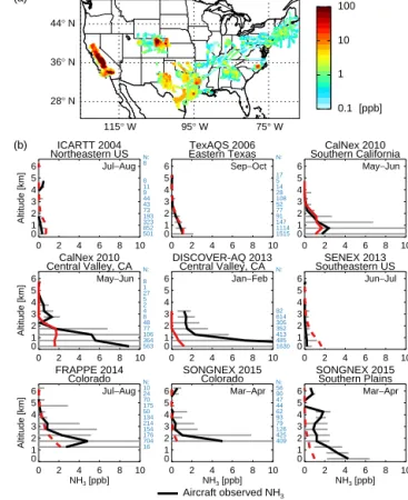
High resolution measurements of ammonia have recently been made in three dimensions aboard aircraft during field campaigns throughout the US. We use data from seven cam-paigns, which we separate into seven regions, for a total of nine snapshots of the vertical distribution of ammonia con-centration. Specific information regarding these cases, in-cluding locations, dates, instrumentation, and uncertainty, is listed in Table 1. All measurements were made with a 1 s interval, except those made during DISCOVER-AQ in Cal-ifornia, which used a 3 s interval, and those made during ICARTT in the northeastern US, which used a 5 s interval. In all cases, the ammonia concentration measurements are averaged to 1 min time resolution. The horizontal spatial dis-tributions of these measurements are shown in Fig. 4a. 3.4 Observed year-to-year ammonia variability
The observed ammonia concentration can be modulated by numerous anthropogenic and environmental factors, includ-ing ammonia emissions, meteorology, and the emission of acid precursors (i.e., SOx and NOx). Emissions of
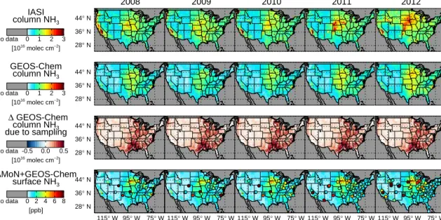
anthro-28° N 36° N 44° N 28° N 36° N 44° N 28° N 36° N 44° N 28° N 36° N 44° N 115° W 95° W 75° W 115° W 95° W 75° W 115° W 95° W 75° W 115° W 95° W 75° W 115° W 95° W 75° W IASI column NH3 GEOS-Chem column NH3 ∆ GEOS-Chem column NH3 due to sampling AMoN+GEOS-Chem surface NH3 2008 2009 2010 2011 2012 [1016 molec cm−2] [1016 molec cm−2] [1016 molec cm−2 ] [ppb] No data 0 1 2 3 No data 0 1 2 3 No data -0.5 0.0 0.5 No data 0 2 4 6 8
Figure 3. Mean summer (JJA) ammonia concentrations for 2008 to 2012 (columns): gridded and filtered IASI observed column concentra-tion, GEOS-Chem simulated column concentration sampled to valid IASI days, changes in GEOS-Chem simulated column concentration due to sampling to coincident IASI measurements, and AMoN observed surface concentration (circles) overlaid on GEOS-Chem surface concentration (rows, top to bottom).
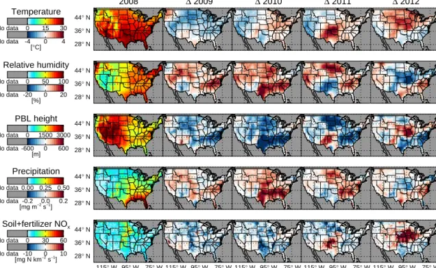
pogenic ammonia are affected by changes in agricultural ac-tivities such as livestock population and fertilizer applica-tion, as well as the implementation of catalytic converters in urban areas. These emissions are sensitive to meteorology that modulates volatilization from the agricultural ammonia sources, increasing with higher temperature and wind speed. Biomass burning events are highly variable and temporar-ily increase ammonia emissions. Our baseline simulation captures only the year-to-year variation in biomass burning emissions of ammonia; emissions from all other sectors are fixed. Meteorology affects the partitioning of ammonia into ammonium nitrate, where higher temperature and lower rel-ative humidity favor the gas phase, as well as the removal of ammonia from the atmosphere by changing the rates of both wet and dry deposition (Russell et al., 1983; Mozurkewich, 1993). Even in a well-mixed boundary layer, ammonia con-centrations may have strong gradients caused by temper-ature variations with altitude that alter gas-to-particle par-titioning of ammonium (Neuman et al., 2003). Figure 5 shows the year-to-year variation in key meteorological pa-rameters across the US from 2008 to 2012 from the GEOS-5 assimilated meteorological product. Emissions of SOxand NOxalso affect the ammonia concentration by regulating the amount of acid available to convert ammonia into ammonium sulfate and ammonium nitrate particles. Figure 1 shows that the anthropogenic component of these emissions decreases substantially in the US during our study period. Meteorology can also affect the rate of soil and fertilizer NOxemissions by changing the storage and volatilization processes (simulated changes also shown in Fig. 5).
Using IASI column concentration and AMoN surface concentration measurements, we show in Fig. 3 that ob-served ammonia concentrations vary significantly from year to year over the US. The mean IASI column concen-tration observed over the US in the summers of 2008 through 2012 is 0.95 × 10¹⁶molec cm−2, which ranges from a low of 0.90 × 10¹⁶molec cm−2 in 2010 to a high of 1.1 × 10¹⁶molec cm−2in 2012 (indicating that the mean am-monia column concentrations over the US range from −5.3 to +16 % of the mean during these 5 years). At the sur-face, the mean AMoN observed ammonia concentration in the summer from all sites with records from 2008 to 2012 is 3.4 ppb, ranging from 3.0 ppb in 2009 to 4.3 ppb in 2012 (or between −11 and +25 % of the mean). The IASI and AMoN observations differ on the year with the lowest mean summer concentration (2010 for IASI and 2009 for AMoN); this difference is likely due to a lack of AMoN sites dis-tributed throughout areas that have low IASI column concen-trations in 2010. The regions of high agricultural production, including California and the Plains, exhibit higher year-to-year variability in the magnitude of IASI column concentra-tions. For example, in the Plains region, maximum summer IASI values are 23 % higher in 2012 than the mean of the 5 study years. This is also the case for surface concentrations at several AMoN sites in the Midwest and the west.
In what follows, we will use the GEOS-Chem model to examine the source of the observed year-to-year variation in ammonia concentrations.
T able 1. Rele v ant details for the observ ed ammonia concentrations sho wn in Fig. 4, including the aircraft campaign, geographic location, dates, ammonia instrument, instrument sample rate, and typical instrument uncertainty range (calibration uncertainty + measurement imprecision), which sho w flight-to-flight v ariability detailed in the respecti v e archi v ed data files. Campaign Re gion (latitude; longitude range) Dates Instrument Uncertainty ICAR TT (No w ak et al., 2007) Northeastern US (38 ◦ N–47 ◦ N; 67–83 ◦ W) Jul–Aug 2004 NH 3 CIMS a ± (30 % + 0.115 ppb) + 0.045 ppb T exA QS (No w ak et al., 2010) Eastern T exas (27–35 ◦ N; 90–100 ◦ W) Sep–Oct 2006 N H 3 CIMS ± (25 % + 0.070 ppb) + 0.035 ppb CalNe x (No w ak et al., 2012) Southern California (CA) (see Schiferl et al., 2014) May–Jun 2010 NH 3 CIMS ± (30 % + 0.200 ppb) + 0.080 ppb CalNe x Central V alle y, California (see Schiferl et al., 2014) May–Jun 2010 NH 3 CIMS ± (30 % + 0.200 ppb) + 0.080 ppb DISCO VER-A Q Central V alle y, California (see Schiferl et al., 2014) Jan–Feb 2013 CRDS b (Picarro G2103) ± (35 % + 1.7 ppb) + 0.2 ppb SENEX Southeastern US (31–43 ◦ N; 75–96 ◦ W) Jun–Jul 2013 NH 3 CIMS ± (25 % + 0.070 ppb) + 0.020 ppb FRAPPE Colorado (38–42 ◦ N; 101–110 ◦ W) Jul–Aug 2014 Aerodyne Dual NH 3 /HNO 3 QCL c ± (22 % + 0.305 ppb) + 0.058 ppb SONGNEX Colorado (38–42 ◦ N; 101–110 ◦ W) Mar –Apr 2015 NH 3 CIMS ± (35 % + 0.500 ppb) + 0.035 ppb SONGNEX Southern Plains (26–36 ◦ N; 93–105 ◦ W) Mar –Apr 2015 NH 3 CIMS ± (35% + 0.500 ppb) + 0.035 ppb a CIMA: chemical ionization mass spectrometer . b CRDS: ca vity ring do wn spectrometer . c QCL: quantum cascade laser . 28° N 36° N 44° N 115° W 95° W 75° W 0.1 1.0 10.0 100.0 [ppb] 0.1 1 10 100 0 2 4 6 8 10 0 1 2 3 4 5 6 Altitude [km] 501 852 323 193 73 43 44 9 11 8 8 N: ICARTT 2004 Northeastern US Jul−Aug (a) (b) 0 2 4 6 8 10 0 1 2 3 4 5 6 1515 1114 147 91 77 52 108 28 14 5 17 N: TexAQS 2006 Eastern Texas Sep−Oct 0 2 4 6 8 10 0 1 2 3 4 5 6 365 1098 552 221 128 126 168 33 5 8 N: CalNex 2010 Southern California May−Jun 0 2 4 6 8 10 0 1 2 3 4 5 6 Altitude [km] 563 364 106 77 48 8 4 2 5 27 1 8 N: CalNex 2010 Central Valley, CA May−Jun 0 2 4 6 8 10 0 1 2 3 4 5 6 1630 485 413 352 305 614 82 N: DISCOVER-AQ 2013 Central Valley, CA Jan−Feb 0 2 4 6 8 10 0 1 2 3 4 5 6 85 2412 531 173 136 113 70 107 31 77 87 32 N: SENEX 2013 Southeastern US Jun−Jul 0 2 4 6 8 10 NH3 [ppb] 0 1 2 3 4 5 6 Altitude [km] 16 704 176 154 214 134 50 175 70 24 10 N: FRAPPE 2014 Colorado Jul−Aug 0 2 4 6 8 10 NH3 [ppb] 0 1 2 3 4 5 6 409 425 126 79 93 62 44 47 90 56 N: SONGNEX 2015 Colorado Mar−Apr 0 2 4 6 8 10 NH3 [ppb] 0 1 2 3 4 5 6 91 792 544 184 51 41 29 17 26 22 6 9 40 N: SONGNEX 2015 Southern Plains Mar−Apr Aircraft observed NH3
GEOS-Chem NH3 Approximate GEOS-Chem NH3
Figure 4. (a) Spatial distribution of 1 min mean observed ammo-nia concentrations for several aircraft campaigns throughout the US listed in Table 1. (b) Vertical profiles of median observed ammo-nia concentration (black) and median GEOS-Chem simulated am-monia concentration (red) averaged in 500 m vertical bins from these campaigns. Simulated concentrations matched to the year and flight tracks of the campaign are shown in solid red, while approx-imately sampled concentrations (mean 2008–2012 simulated con-centrations) are shown in dashed red. Gray bars show the standard deviation of observations in each bin. The number of observations in each bin are shown in blue. The 2 months during which the cam-paign took place are indicated in the top right of each profile.
4 Base scenario simulation of ammonia measurements Throughout this section, we use the GEOS-Chem model to investigate how well the model captures the observed magni-tude and variability in ammonia concentrations. We sample the model to simulate the ammonia concentrations observed in both temporal and spatial dimensions.
4.1 Column comparison
To evaluate the ammonia concentration throughout the col-umn, the simulated column concentrations are recorded at the local 09:00–10:00 overpass time, and this 1 h mean is compared to the IASI retrievals at 09:30 local time. It is not straightforward to compare this value in an unbiased way with the IASI measurements since the vertical
sen-28° N 36° N 44° N 28° N 36° N 44° N 28° N 36° N 44° N 28° N 36° N 44° N 28° N 36° N 44° N 115° W 95° W 75° W 115° W 95° W 75° W 115° W 95° W 75° W 115° W 95° W 75° W 115° W 95° W 75° W Temperature Relative humidity PBL height Precipitation Soil+fertilizer NOx 2008 ∆ 2009 ∆ 2010 ∆ 2011 ∆ 2012 [°C] [%] [m] [mg m−2 s−1] [mg N km−2 s−1 ] No data 0 15 30 No data -4 0 4 No data 0 50 100 No data -20 0 20 No data 0 1500 3000 No data-600 0 600 No data0.00 0.25 0.50 No data -0.2 0.0 0.2 No data 0 30 60 No data -10 0 10
Figure 5. Mean summer (JJA) assimilated GEOS-5 meteorology parameters and meteorologically driven NOxemissions used in
GEOS-Chem simulation for 2008 to 2012 (columns): temperature, relative humidity, planetary boundary layer (PBL) height, precipitation, and
soil + fertilizer NOxemissions (rows, top to bottom). Absolute values for 2008 shown along with changes from 2008 for 2009 to 2012.
sitivity of the instrument may not be consistent with the model. For this reason, this value cannot be quantitatively compared to the IASI retrieved column with confidence; however, we qualitatively compare trends and spatial fea-tures here. When sampling is applied, only simulated days with valid IASI retrievals (at least one per grid box) are in-cluded. Seasonal means are calculated as the mean of all days (no sampling) or of only days with valid IASI re-trievals (with sampling). The simulated ammonia column concentrations are generally well correlated with the IASI observations (Fig. 6) over the summer, particularly in the Plains and the Midwest (correlation (R) = 0.6–0.8). Sam-pled simulated column concentrations shown in Fig. 3 have a summer mean of 0.64 × 10¹⁶molec cm−2, ranging from 0.52 × 10¹⁶molec cm−2in 2009 to 0.80 × 10¹⁶molec cm−2 in 2012 (or between −19 and +25 % of the mean). We find considerable year-to-year variation in the simulated ammo-nia concentration, even with fixed ammoammo-nia emissions.
Sampling the model to match IASI observations, as shown in Fig. 3, increases the concentrations in regions with more invalid IASI days according to the filtering process described in Sect. 3.1. Valid days tend to have higher concentrations as they meet the filter requirements due to more favorable retrieval conditions, which include a higher retrieved am-monia signal. Cloudy days, being cooler and having greater probability of rain, also tend to have lower ammonia con-centrations, and these cannot be retrieved. In the
southeast-28° N 36° N 44° N
115° W 95° W 75° W No data-1.0 -0.5 0.0 0.5 1.0R
Figure 6. Summer (JJA) correlation (R) for all years (2008–2012) between daily gridded and filtered IASI ammonia column concen-tration and daily GEOS-Chem base scenario ammonia column con-centration.
ern US, sampling increases the regional summer mean sim-ulated ammonia column concentration significantly, by 26 % (2011) to 58 % (2012). Even after accounting for this sam-pling bias, the simulated column concentrations are tently lower than those observed by IASI, which is consis-tent with the findings of Van Damme et al. (2014b) over Eu-rope. This underestimate is because the filter requirement re-stricting high relative error inherently favors larger observed columns. Consequently, there is lower year-to-year variabil-ity in the mean summer IASI column concentrations (21 % of the mean between the highest and lowest years) than those simulated by the model (44 %). This discrepancy in variabil-ity may also be due to our use of total column values, rather
than isolating the layers where the satellite has greater sensi-tivity. For example, removing the more variable near-surface layers, where the satellite is presumed to be less sensitive, could reduce the model variability in the comparison men-tioned above.
The distribution of ammonia throughout the column is also relevant to assessing the ability of the model to represent the ammonia column concentration observed by IASI, as the re-trieval has varying sensitivity at different vertical levels. In Fig. 4b we use measurements of ammonia from several air-craft campaigns throughout the US to evaluate the simulated ammonia vertical profile. We show the median, rather than the mean, to account for the inherent inability of the model to reproduce highly concentrated plumes occasionally ob-served by the aircraft. To compare the observations with the simulation during campaigns that take place in our study pe-riod (extended to February 2013), we sample the model di-rectly in time and space for each flight of the campaign. For campaigns outside of this time period, we sample directly in space for each flight but approximate the time compo-nent by using the 5-year mean (2008–2012) of each 2-month campaign window. As shown in Fig. 4b, the observed me-dian ammonia vertical profile is highly variable in magnitude and shape between different regions. In high ammonia emis-sion regions, the observed ammonia concentration increases greatly toward the surface, and the median ammonia verti-cal profile is less variable between different campaigns in the same region (e.g., Central Valley in 2010 and 2013, Col-orado in 2014 and 2015) than between different regions. As with the observations, the model performance varies greatly between regions. Over areas such as Central Valley, previ-ously examined by Schiferl et al. (2014), the model underes-timates ammonia throughout the vertical profile, especially near the surface. The model also performs more poorly in the spring according to measurements in Colorado and the southern Plains in 2015, but limited sampling across seasons makes it difficult to be conclusive. Other regions, like south-ern California, eastsouth-ern Texas, Colorado in summer 2014, and the southeastern US have a much smaller bias. The slight high bias in the model at the surface in the northeastern and southeastern US regions is consistent with previous evalu-ation of NEI-2005 in GEOS-Chem against AMoN measure-ments (Paulot et al., 2014). Local conditions clearly influence the model simulation of the observed concentrations. Over-all, the model shows less variability than the observations, but the model profile shape is generally consistent with the observed shape outside of large source regions. This sug-gests that, outside of these source regions, model biases in the shape of the vertical profile are unlikely to bias compar-isons with satellite column observations.
4.2 Surface comparison
Summer seasonal mean simulated surface concentrations are compared with the seasonal mean AMoN surface
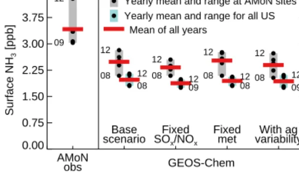
concentra-0.00 0.75 1.50 2.25 3.00 3.75 4.50 Surface NH 3 [ppb] 09 12 08 12 08 12 08 12 08 12 GEOS-Chem AMoN obs Base
scenario SOFixedx/NOx
Fixed
met variabilityWith ag
08 12 09 12 08 12 09 12 Yearly mean and range at AMoN sites
Mean of all years
Yearly mean and range for all US
Figure 7. Yearly summer (JJA) mean surface ammonia concentra-tion (black circles) and mean of all years (red bar) for observed AMoN sites valid from 2008 to 2012 and four GEOS-Chem
scenar-ios: base scenario, fixed anthropogenic SOx and NOx emissions,
fixed meteorology, and including agricultural ammonia emission variability (left to right). Vertical bars indicate the range of all years: simulation sampled to AMoN sites (gray) and simulation for the en-tire US (blue).
tion observations in Fig. 3. For a more direct comparison of individual observations, we match the hours of the AMoN sampling period with the corresponding hourly values from the simulation, and the mean of these hours is used for com-parison. We also apply a spatial interpolation scheme to this comparison, where the four nearest grid box values are aver-aged based on the distance between their center and the ob-servation site location. This adjusts the simulated concentra-tion to account for the influence of nearby grid boxes at sites near grid box edges and in regions that exhibit strong hori-zontal gradients. The mean summer simulated surface con-centration at AMoN sites with measurements from 2008 to 2012 (11 sites) is 2.5 ppb, which varies from a low of 2.1 ppb in 2008 (−16 % of the mean) to a high of 2.8 ppb in 2012 (+13 % of the mean) over the study time period. This mean simulated concentration is lower than that observed (2.5 ppb vs. 3.4 ppb). The range of simulated surface concentrations between high and low years is also half of the range ob-served (0.73 ppb vs. 1.3 ppb). These ranges are shown for comparison in Fig. 7 along with the range in surface ammo-nia concentrations over the entire US. The range in summer-time mean ammonia concentrations across the US is smaller, and the mean is lower (by more than 25 %) than when sam-pled to the AMoN sites. This suggests that the AMoN net-work does not adequately represent the range of ammonia concentrations across the US; as many AMoN sites are lo-cated near high ammonia source regions, there is a sampling bias for this network. The near-source location of many of these AMoN sites provides an additional challenge for the regional-scale resolution model simulation used here and is likely responsible for some of the model underestimate.
By limiting the above analysis to only summers 2011 and 2012, the number of sites with measurements in both years increases to 48. The mean bias in this case is more modest
(−0.02 ppb), with 2011 biased slightly high and 2012 biased slightly low. There is a consistent high bias at many of the eastern US sites, which is offset by a low bias in the west in 2012, likely due to local biomass burning that is not ade-quately captured in the model. However, even for this limited time period, the model fails to reproduce the observed year-to-year variation (observed 0.80 ppb increase in the summer-time mean from 2011 to 2012, with a simulated increase of only 0.11 ppb). This difference is dominated by high mea-surements in 2012 in the west, but the observed increase from 2011 to 2012 in the Midwest is also underestimated.
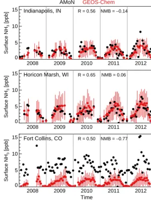
Figure 8 shows a detailed comparison of observed and base scenario simulated surface ammonia concentrations at three AMoN sites with records from 2008 to 2012; these are selected as representative regional sites and demonstrate the varying degree of model skill. Simulated concentrations at all three sites reproduce the observed seasonal cycle, with high-est concentrations in the summer and lowhigh-est in the winter. The Indianapolis, Indiana, site represents typical Midwest-ern sites, with nearby urban SOx and NOxemission sources surrounded by rural ammonia sources. This site is located in central Indianapolis, and the corresponding model grid box is made up of about 30 % city and 60 % rural land. The over-all comparison at Indianapolis is good throughout the study period, with an R of 0.56 and a normalized mean bias (NMB) of −0.14 (mean bias of −0.41 ppb). There is a noticeable in-creasing trend in the observed ammonia concentrations from 2008 to 2012; the model captures much of this upward trend. The Horicon Marsh, Wisconsin, site represents rural re-gions where ammonia emissions are primarily from agri-cultural sources. This site is located in a grid box that is nearly 90 % farm land (the remaining 10 % is made up of small towns and wetlands). This uniformity should be eas-ier for the model to represent. The comparison between ob-served and simulated ammonia concentration is generally very good when considering the entire time period (R = 0.65, NMB = 0.06, mean bias = +0.19 ppb). However, this com-parison is somewhat worse in the summer (R = 0.44), as the model does not properly simulate the timing or magnitude of the peak concentrations.
Finally, the Fort Collins, Colorado, site represents one of several sites in the western US that present a challenge to simulate due to large horizontal concentration gradients over areas with highly varying topography. This is an area of high livestock ammonia emissions to the east bounded on the west by the Front Range of the Rocky Mountains. Ammonia is ad-vected from feedlots to the east and observed high concentra-tions result. The site is located on the eastern side of a grid box that is made up of 75 % mountains and forest toward the west. There is considerable elevation increase as well from east to west. As a result, simulated concentrations in this grid box take on the characteristics of the mountain region rather than the agricultural plain. There is a large low bias at the Fort Collins site of −4.7 ppb (R = 0.50, NMB = −0.77) for the entire time period. If we compare the observations
0 5 10 15 Surface NH 3 [ppb] 2008 2009 2010 2011 2012 Indianapolis, IN R = 0.56 NMB = −0.14 AMoN GEOS-Chem 0 5 10 15 Surface NH 3 [ppb] 2008 2009 2010 2011 2012 Horicon Marsh, WI R = 0.65 NMB = 0.06 0 5 10 15 Surface NH 3 [ppb] 2008 2009 2010 2011 2012 Time Fort Collins, CO R = 0.50 NMB = −0.77
Figure 8. Observed (black circles) and base scenario simulated (red circles) surface ammonia concentration time series at three AMoN sites from 2008 to 2012: Indianapolis, Indiana (IN) (top, urban), Horicon Marsh, Wisconsin (WI) (middle, agricultural), and Fort Collins, Colorado (CO) (bottom, varying topography/high horizon-tal gradient). Standard deviation of simulated hours shown as ver-tical red lines. Gray verver-tical lines indicate the transition between calendar years.
with simulated values of the next grid box east in the agricul-tural region (without weighting neighboring grid boxes), the bias drops significantly (about 35 %), so that only −3.0 ppb bias in all months remains. However, even with this adjust-ment to account for site location, the model performance here is among the poorest. Similar comparisons for the eight re-maining sites with records during this time period are shown in Figs. S1–S3 in Supplement.
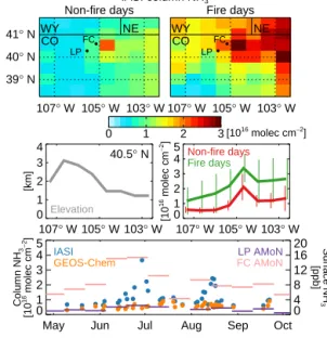
4.3 Integrated comparison: Colorado, summer 2012 The variation of both the observed column and surface am-monia concentrations in the western US is influenced by biomass burning events in the summer of 2012. The wild-fire activity in the Colorado Front Range during this time (May–September 2012) provides an opportunity to synthe-size the different ammonia concentration information dis-cussed above as this is an area that is also known for high agricultural ammonia emissions.
IASI measurements during days without fire emission in-fluence (determined by visual inspection of Moderate Res-olution Imaging Spectroradiometer (MODIS) imagery, with at least 75 % domain retrieval coverage) show a peak mean
column concentration of 2.1 × 10¹⁶molec cm−2 just to the east of Fort Collins (FC) (Fig. 9), corresponding to the loca-tion of feedlots. The mountains to the west of FC, along with ridges to the north and south, cause the agriculturally emit-ted ammonia to circulate throughout the Front Range, with only limited transport westward (Wilczak and Glendening, 1988). Column concentrations remain elevated to the south and east throughout the plain of eastern Colorado, while concentrations in western areas of the domain at high el-evations are quite low. Aircraft measurements in Colorado during the FRAPPE (summer 2014) and SONGNEX (spring 2015) campaigns confirm this distribution of ammonia in the region (Fig. 4a). Figure 9 shows that IASI column concentra-tions are considerably higher on days with wildfire activity. The largest increase takes place over the Front Range near FC and to the east due to fires located in the Colorado moun-tains during late June–early July, when the mean IASI col-umn over the region more than doubles. In August, colcol-umn concentrations are enhanced in the north and west of the do-main due to the transport of wildfire plumes into the region from fires in other areas of the northwestern US. Thus, we see in Fig. 9 that the average ammonia concentrations ob-served by IASI during the season are elevated throughout the region due to fire emissions. These wildfire emissions are present in addition to the persistent agricultural ammo-nia sources throughout the time period, as the feedlot grid box east of FC has the highest column concentration even on wildfire-influenced days (3.4 × 10¹⁶molec cm−2, increase of 62 %). However, the IASI retrieval is more sensitive to am-monia lofted vertically, as is the case in biomass burning outflow. The GEOS-Chem simulated ammonia column con-centrations in this domain do not capture the peaks observed by IASI throughout the time period. This suggests that the model inventory underestimates the fire emissions of ammo-nia or their injection height; these biases are likely exacer-bated by the IASI vertical sensitivity.
AMoN surface concentrations at the FC site, also in Fig. 9, follow the peaks in concentration observed by IASI in both June and August and show a similar relative increase (fac-tor of ∼ 2 in late June), while surface concentrations at the Longs Peak (LP) AMoN site show no evidence of an en-hancement due to fire, likely because the site is isolated from the Front Range source region. It is difficult to quantify the contribution of the wildfire ammonia source from these ob-servations because the fire events also correspond to the high-est surface temperatures of the year, thereby affecting ammo-nia volatilization and partitioning chemistry. Additional ob-servations of ammonia concentrations in fire plumes could help improve emissions estimates and clarify the importance of this source (e.g., Whitburn et al., 2015).
4.4 Updated inventory comparison
A more recent anthropogenic emission inventory, NEI-2011, is available over the US for 2011
(avail-39° N 40° N 41° N 107° W 105° W 103° W CO WY NE LP FC 107° W 105° W 103° W CO WY NE LP FC 0 1 2 3[1016 molec cm−2 ]
Non-fire days Fire days
IASI column NH3 107° W 105° W 103° W 0 1 2 3 4 [km] Elevation 40.5° N 107° W 105° W 103° W 0 1 2 3 4 5 Non-fire days Fire days [10 16 molec cm − 2]
May Jun Jul Aug Sep Oct
0 1 2 3 4 5 0 4 8 12 16 20 Column NH 3 [10 16 molec cm − 2] Surface NH 3 [ppb] IASI GEOS-Chem LP AMoN FC AMoN
Figure 9. Mean gridded IASI column ammonia concentration over the Colorado Front Range from May to September 2012 during non-fire days (top left) and fire days (top right). Elevation of each
grid box center at 40.5◦N over the longitude range above
(mid-dle left). Mean IASI column ammonia concentration at each grid
box at 40.5◦N over the longitude and time range above for
non-fire days (red) and non-fire days (green) (middle right). Mean daily IASI (blue) and GEOS-Chem (orange) column ammonia concentrations over the domain above and observed surface ammonia concentra-tions at the Longs Peak (LP) (purple) and Fort Collins (FC) (pink) AMoN sites (bottom).
able from www.epa.gov/air-emissions-inventories/ 2011-national-emissions-inventory-nei-data, adapted for GEOS-Chem by Travis et al., 2016). This inventory includes changes in both the magnitude and timing of anthropogenic ammonia, SOx, and NOx when compared to NEI-2005. Averaged over the summers during the study period of 2008 to 2012, anthropogenic ammonia emissions are 26 % higher, anthropogenic SOx emissions are 13 % higher, and anthropogenic NOxemissions are 11 % lower in NEI-2011 compared to in NEI-2005 as applied to GEOS-Chem over the US. Variable spatial seasonality for ammonia emissions has been included in NEI-2011 such that known emissions events like springtime fertilizer application in the Midwest are now accounted for.
We repeat our GEOS-Chem simulations with NEI-2011 for 2008 and 2012 and compare the simulated surface con-centrations with the observed AMoN surface concentration in these 2 years. Generally, the summer high concentration bias at the eastern US sites is reduced using the updated in-ventory. The simulation improves at a few of the western sites as well, but many biases remain or worsen. Strong gradients in local sources and geography still likely play a large role at many of these sites. At Midwestern sites, the new sea-sonality often better represents the springtime and summer
peak concentration, but the comparison during the transition to late summer and fall is degraded. For Horicon Marsh, Wis-consin, the summer R in 2008 and 2012 between observed and simulated surface concentrations decreases from 0.63 to 0.48 when using NEI-2011 rather than NEI-2005. While NEI-2011 may better represent the magnitude and timing of emissions in some locations, it is also a year-specific inven-tory and does not provide a better constraint than NEI-2005 on the year-to-year variations in ammonia emissions that are the main focus of this study.
4.5 Summary of base scenario to observation comparisons
From the comparisons described here, we conclude that the model generally captures the vertical, temporal, and regional variability of ammonia but underestimates the summertime ammonia concentration observed in both the column and at the surface, particularly near source regions (including both agricultural and fire emissions). The year-to-year variability in the model at the surface is lower than the variability ob-served, but the trends and variability captured by the sim-ulation are significant considering that ammonia emissions in the model are fixed. We next explore the processes in the model that contribute to this variability.
5 Attributing sources of ammonia variability 5.1 SOxand NOxemissions reductions
In order to identify the drivers of year-to-year variation in simulated ammonia concentrations, we run sensitivity stud-ies that isolate individual factors affecting the ammonia con-centrations. The first sensitivity simulation holds anthro-pogenic SOxand NOxemissions constant at 2008 levels for 2009 to 2012 in order to gauge the effects of these emis-sions reductions on the ammonia concentration in the base scenario. This analysis relies on an accurate simulation of the trends in sulfate and nitrate in areas of significant ammonia concentration. Briefly, we evaluate our base scenario against observations from all available sites (148) in the Interagency Monitoring of Protected Visual Environment (IMPROVE) network (vista.cira.colostate.edu/improve) over our study pe-riod. Comparison of the trend in summer mean indicates that GEOS-Chem reproduces well the decreasing trend in sul-fate over the eastern US and the Pacific coast (not shown). In the Intermountain West, which generally lacks high am-monia concentrations, the simulation predicts a decreasing trend in sulfate, while the observations show an increase. The model generally reproduces the trend in nitrate, although the decline in nitrate in the eastern US is somewhat stronger than observed. This indicates a possible oversensitivity to chang-ing NOxemissions in the model.
Figure 10 shows that SOxand NOxreductions over the US act to significantly increase the ammonia column
concentra-tion over time. Much of this increase takes place over the eastern US, where anthropogenic SOx and NOx emissions are highest (Fig. 1), and therefore where absolute reductions in SOx and NOx are largest. Decreases in the sulfate and total nitrate (TNO3=HNO3+NO−3)availability caused by the SOx and NOxemission reductions, respectively, require less ammonium to neutralize particle-phase acids, leaving more ammonia in the gas phase. For the US summer mean, the simulated ammonia surface concentrations increase by 8.8 % from 2008 to 2012 due to the anthropogenic emissions changes, compared to the 29 % decrease in total SOx emis-sions and the 17 % decrease in total NOxemissions. We at-tribute 32 % (0.17 ppb) of the range of summer surface am-monia concentration simulated by the base scenario to an-thropogenic SOx and NOx emissions reductions. In the col-umn, 26 % (0.07 × 10¹⁶molec cm−2)of the range is due to these reductions.
5.2 Meteorology variability
The second sensitivity simulation tests the effects that me-teorological variability has on the simulated ammonia con-centration. In this simulation, we hold the GEOS-5 assim-ilated meteorology constant at year 2008 conditions for all years of our simulation (2008–2012). Meteorology can al-ter the distribution and phase of ammonia via changes in transport, deposition, oxidation, and gas-particle partition-ing. Soil and fertilizer NOx emissions are also effectively held constant in this simulation given that their variability is largely controlled by meteorology. While meteorology may indirectly affect biomass burning emissions, such as by lead-ing to more fires durlead-ing a dry and hot year, we do not account for this here, as these emissions are allowed to vary in all cases. Comparison with both 10- and 35-year mean Modern-era Retrospective Analysis for Research and Applications (MERRA) meteorology from the NASA GMAO (Rienecker et al., 2011) shows that 2008 is a typical meteorological year in the US. Thus, anomalies from 2008 in 2009–2012 can be seen as realistic deviations from an average condition.
Figure 10 shows that the effects of meteorology on the ammonia concentration are highly variable both spatially and temporally. The spatial variability is generally greater at the surface (not shown) than in the column. Variations in simulated ammonia concentration can be connected with the meteorological features shown in Fig. 5. For exam-ple, the summer of 2010 in the southeastern US is a high-precipitation year that contributed to lower ammonia concen-tration throughout the column due to increased wet removal. Higher relative humidity also likely contributes to this de-crease by favoring the particle phase of the ammonium ni-trate equilibrium. Another example is the high-temperature, low-humidity and low-precipitation summer of 2012 in the Plains and the Midwest, which favors the gas phase of the ammonium nitrate equilibrium and generally higher concen-trations (due to reduced removal). However, these same high
28° N 36° N 44° N 28° N 36° N 44° N 28° N 36° N 44° N 115° W 95° W 75° W 115° W 95° W 75° W 115° W 95° W 75° W 115° W 95° W 75° W 2009 2010 2011 2012 ∆ GEOS-Chem column NH3
due to SOx/NOx reductions
∆ GEOS-Chem column NH3
due to meteorology variability
∆ GEOS-Chem column NH3
due to partitioning variability [1016 molec cm−2 ] [1016 molec cm−2 ] [1016 molec cm−2 ] No data -0.5 0.0 0.5 No data -0.5 0.0 0.5 No data -0.5 0.0 0.5
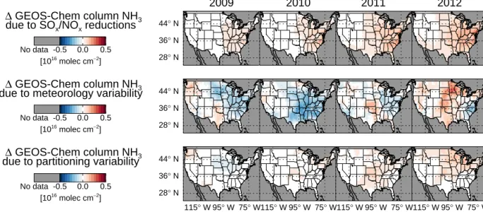
Figure 10. Simulated mean summer (JJA) ammonia column concentration changes for 2009 to 2012 (columns) caused by anthropogenic
SOx and NOx emissions reductions, assimilated meteorology variability, and meteorology variability affecting only ammonium nitrate
partitioning (rows, top to bottom). Compare to the baseline ammonia column shown in Fig. 3.
temperatures in 2012 lead to higher emissions of soil and fer-tilizer NOx, which modestly counteract this effect at the sur-face by encouraging more ammonia to partition to the par-ticle phase to neutralize this supply of acid (Fig. 5). Lower planetary boundary layer (PBL) heights, such as in the upper Midwest in summer 2011, can trap ammonia near the sur-face. More ammonia nearer the surface could increase the dry deposition flux as this is the primary direct removal method for gaseous ammonia, slightly offsetting the increased con-centration due to trapping and decreasing the concon-centration throughout the column. We attribute 64 % (0.34 ppb) of the range of summer surface ammonia concentration simulated by the base scenario to meteorology. In the column, 67 % (0.18 × 10¹⁶molec cm−2)of the range is due to these ations. Meteorology clearly dominates the year-to-year vari-ability in simulated ammonia concentration.
A third sensitivity simulation isolates the effects of two-way partitioning of ammonia on the simulated ammonia con-centration. This partitioning is driven by the ambient tem-perature and relative humidity as inputs into ISOROPPIA II. In this simulation, we hold these inputs constant at year 2008 conditions for all years of our simulation (2008–2012). Higher temperature and lower relative humidity generally fa-vor partitioning into the gas phase and an increase in ammo-nia concentration. The results of this simulation, shown in Fig. 10, indicate that the effects of partitioning are less spa-tially and temporally variable than those of all meteorology discussed above. The variability due to partitioning can make up a significant portion of the change due to all meteorology, such as in the warm summer of 2012 when partitioning ac-counts for 73 % of the net change due to all meteorology. This is also true to a smaller degree during the cool summer
of 2009 (13 %). In relatively wet summers, such as 2010 and 2011, enhanced partitioning acts to offset the losses due to all meteorology (likely caused by increased wet deposition) by 10 and 73 %, respectively. Overall, partitioning accounts for 23 % (0.06 × 10¹⁶molec cm−2)of the range in the sum-mer base scenario column concentrations, which is 33 % of the range due to all meteorology. Thus, the phase partition-ing due to meteorology plays a significant, but not always dominant, role in controlling the variability of ammonia. 5.3 Missing simulated ammonia variability
The simulated ammonia concentrations do show significant year-to-year variability despite constant ammonia emissions, but this variability is generally lower than that observed by IASI and AMoN at individual locations (Figs. 3 and 7). How-ever, maximum observed column concentrations in the west-ern US in 2012 are likely from smoke enhancements at the vertical levels at which IASI is more sensitive; the model cannot reproduce this column variability without properly weighting the different vertical levels sensitive to these con-centrations. There are also not enough AMoN sites over the entire time period to robustly indicate either regional varia-tions in surface ammonia concentration or whether a partic-ular site is impacted by local emission changes. The range of simulated mean ammonia concentrations is 0.53 ppb less than the range observed at the available sites over the sum-mers of 2008 to 2012 (Fig. 7). Most of this missing range is from sites in the west and the Midwest, where agricultural ammonia emissions are higher. The observed range is likely influenced by high biomass burning emissions in the west and high temperature effects on partitioning in the Plains and the Midwest, which are greater than in the model. In addition,