HAL Id: hal-02510833
https://hal.sorbonne-universite.fr/hal-02510833
Submitted on 18 Mar 2020
HAL is a multi-disciplinary open access archive for the deposit and dissemination of sci-entific research documents, whether they are pub-lished or not. The documents may come from teaching and research institutions in France or abroad, or from public or private research centers.
L’archive ouverte pluridisciplinaire HAL, est destinée au dépôt et à la diffusion de documents scientifiques de niveau recherche, publiés ou non, émanant des établissements d’enseignement et de recherche français ou étrangers, des laboratoires publics ou privés.
Advancing quantitative understanding of self-potential
signatures in the critical zone through long-term
monitoring
Kaiyan Hu, Damien Jougnot, Qinghua Huang, Majken Looms, Niklas Linde
To cite this version:
Kaiyan Hu, Damien Jougnot, Qinghua Huang, Majken Looms, Niklas Linde. Advancing quantitative understanding of self-potential signatures in the critical zone through long-term monitoring. Journal of Hydrology, Elsevier, 2020, 585, pp.124771. �10.1016/j.jhydrol.2020.124771�. �hal-02510833�
1
Advancing quantitative understanding of self-potential signatures in
the critical zone through long-term monitoring
Kaiyan Hu
1,2, Damien Jougnot
3, Qinghua Huang
1, Majken C. Looms
4,
Niklas Linde
2,*1Department of Geophysics, Peking University, 100871 Beijing, China
2Institute of Earth Sciences, University of Lausanne, 1015 Lausanne Switzerland 3Sorbonne Université, CNRS, EPHE, UMR 7619 Metis, F-75005, Paris, France 4Department of Geosciences and Natural Resource Management, University of
Copenhagen, Øster Voldgade 10, 1350 Copenhagen, Denmark
* Corresponding author. E-mail address: niklas.linde@unil.ch
Author contact:
Kaiyan Hu: huk@pku.edu.cn; kaiyan.hu@unil.ch
Damien Jougnot: damien.jougnot@upmc.fr
Qinghua Huang: huangq@pku.edu.cn
Majken C. Looms: mcl@ign.ku.dk
Niklas Linde: niklas.linde@unil.ch
This paper has been accepted for publication in Journal of Hydrology:
K. Hu, D. Jougnot, Q. Huang, M. C. Looms, N. Linde (2020), Advancing quantitative understanding of self-potential signatures in the critical zone through long-term monitoring, Journal of Hydrology, 585, 124771, doi: 10.1016/j.jhydrol.2020.124771
2 ABSTRACT
The self-potential (SP) method is a passive geophysical technique, which may offer
insights about water and ionic fluxes in the vadose zone. The main obstacles presently
prohibiting its routine use in quantitative vadose zone hydrology are the superposition
of signals arising from various source mechanisms, difficult-to-predict electrode
polarization effects that depend on electrode design and age, as well as water saturation,
pore water chemistry, clay content, and temperature in the immediate vicinity of the
electrodes. We present a unique long-term SP monitoring experiment focusing on the
first four years of data acquired at different depths in the vadose zone within the HOBE
hydrological observatory in Denmark. Using state-of-the-art SP theory combined with
flow and transport simulations, we attempt to replicate the observed data and suggest
reasons for observed discrepancies. The predictions are overall satisfactory during the
first six months of monitoring after which both the patterns and magnitudes of the
observed data change drastically. Our main observations are (1) that predicted SP
magnitudes are strongly sensitive to how the effective excess charge (or alternatively,
the voltage coupling coefficient) scales with water saturation implying that continued
research is needed to build more accurate models of electrokinetic phenomena in
unsaturated conditions, (2) that significant changes in electrode polarization occur in
the shallowest electrodes at time scales of a year, most likely due to desaturation by
capillarity of the fluids filling the electrodes, suggesting that electrode effects cannot
3
monitoring studies, and (3) that multi-rate mass transfer and reactive transport modeling,
with specific emphasis on fluid-mineral interactions, are needed to better predict
salinity and pore water conductivity. We hope to stimulate other researchers to test new
SP modeling approaches and interpretation strategies against these data by making the
SP and complimentary (temperature, dielectric constant, potential/actual
evapotranspiration, precipitation) data time-series available.
Keywords: Hydrogeophysics; Long-term monitoring; Self-potential; Vadose zone;
4 1. Introduction
Self-potential (SP) signals are mainly generated by naturally-occurring
electrokinetic, electrochemical and bioelectrical source mechanisms (Revil and Jardani,
2013). In the SP method, passive measurements with non-polarizing electrodes are used
to map or monitor voltages on the ground surface or in boreholes. Due to a rich set of
natural source mechanisms, the SP method has been used to study a wide range of
hydrological and critical zone processes. Most studies have based their interpretations
on the electrokinetic effect, which originates when water flowing in porous media drags
excess electric charges in the electrical double layer to produce the so-called streaming
potential. SP signals attributed to streaming potentials have been used to characterize
hydraulic parameters (e.g., Zlotnicki and Nishida, 2003; Jardani et al., 2009; Jougnot et
al., 2012; Soueid Ahmed et al., 2014), landslides (Lapenna et al., 2003) and seepage
from dams (e.g., Ikard et al., 2014; Rittgers et al., 2014; Soueid Ahmed et al., 2019). SP
signals of electrochemical origin arise in the presence of ionic concentration gradients
in the pore water or when redox reactions are facilitated by electronic conductors.
Self-potential signals of electrochemical origin have been used to constrain saline tracer and
contaminant transport (e.g., Maineult et al., 2005; Martínez-Pagán et al., 2010; Jougnot
et al., 2015), sea water intrusion (e.g., Graham et al., 2018; MacAllister et al., 2018), to
locate the corrosion of buried metallic bodies (e.g., Castermant et al., 2008; Rittgers et
al., 2013) and to invert for redox maps associated with contaminant plumes (Linde and
5
not only comprise information about subsurface processes of interest such as water and
solute fluxes in the vadose zone. The recorded voltages are also adversely affected by
electrode-related effects (Petiau and Dupis, 1980; Perrier et al., 1997; Petiau, 2000;
Jougnot and Linde, 2013) and external sources originating from telluric currents and
man-made electrical and electromagnetic installations (Perrier et al., 1997; Park et al.,
2007; DesRoches and Butler, 2016).
Self-potential monitoring data contain transient effects, as well as more periodic
short- and long-term variations of different origins. In the literature, SP data are often
interpreted in terms of one process of primary interest, while other possible effects and
time-scales are ignored or filtered out. Despite a large number of published SP studies,
only few have concerned longer-term monitoring (Perrier et al., 1997; Doussan et al.,
2002; Voytek et al., 2019). Here, we investigate four years of SP monitoring data
acquired with permanently installed electrodes at different depths within the vadose
zone at the HOBE hydrological observatory (www.hobecenter.dk) in Denmark. Our
emphasis is on understanding the main signatures of the observed SP data and to
highlight effects that currently limit our ability to make quantitative predictions about
vertical water and solute fluxes in the vadose zone. Instead of filtering out unwanted
effects such as electrode offsets and quasi-linear drifts, we attempt to use the SP record
in its entirety to truly understand to what extent the SP method can be used as a
predictive tool in vadose zone and critical zone science. For instance, can SP monitoring
data be used in a reliable manner to estimate in situ water fluxes in the vadose zone?
6
depth are directed upward or downward? We contrast the measured SP data with
state-of-the-art SP numerical modeling that accounts for electrokinetic and electrochemical
contributions, as well as electrode effects. In an effort to engage the SP community in
research towards an improved mechanistic and quantitative understanding of SP signals
in the critical zone, we make the full SP and complimentary (dielectric constant,
temperature, potential and actual evapotranspiration, precipitation) data record
available.
2. Methodology
Section 2.1 introduces basic self-potential theory followed by more detailed
sections describing the electrokinetic contribution (section 2.1.1), the electro-diffusive
contribution (section 2.1.2), and electrode-effects (section 2.1.3) leading to the total SP
response (section 2.1.4). Section 2.2 introduces the hydrodynamic characterization and
modeling that is needed input for self-potential modeling in the vadose zone. Water
flow and solute transport (section 2.2.1) is first introduced before explaining how in
situ field data are used to infer vadose zone properties by inversion (section 2.2.2).
2.1. Self-potential theory
Below we describe the theory used to perform numerical simulations of SP signals
in the vadose zone. In this treatment, we exclude the redox contribution since we do not
expect electronic conductors at the HOBE site.
7
∇ ∙ 𝐉𝐭𝐨𝐭 = ∇ ∙ (𝐉𝐜+ 𝐉𝐞𝐤+ 𝐉𝐞𝐝+ 𝐉𝐞𝐞) = 0, (1)
where the total electric current density 𝐉𝐭𝐨𝐭 is the sum of the conductive current density
𝐉𝐜 (A/m2) , the electrokinetic current density 𝐉
𝐞𝐤 (A/m2) and the electro-diffusive
current density 𝐉𝐞𝐝 (A/m2) and electrode-related contributions 𝐉
𝐞𝐞 (A/m2) . The
conductive current density 𝐉𝐜 (A/m2) obeys Ohm’s law:
𝜎(𝜃w)𝐄 = 𝐉𝐜, (2)
where 𝐄 (V/m) is the electric field, which is the negative gradient of electrical
potential 𝜑 (V), 𝜎(𝜃w) (S/m) is the effective electrical conductivity of the soil. For
coarser soils without fines, we have (Archie, 1942) :
𝜎(𝜃w) = 𝐹−1𝜎w𝑆𝑤𝑛, (3)
where 𝑆𝑤 = 𝜃w
𝜙 is the water saturation, 𝜃w is the water content, 𝐹 = 𝜙
−𝑚 is the
formation factor, 𝜙 is the porosity, 𝑚 is the cementation exponent and 𝑛 is the
saturation exponent. For soils containing fines, the relationship between bulk electrical
conductivity and pore water electrical conductivity is rather complex and non-linear
(e.g., Revil et al., 2019). Assuming that the pore water is a NaCl-solution, the electrical
conductivity of pore water 𝜎w (S/m) , the temperature of water 𝑇 (℃) and solute
8 𝜎w = (5.6 + 0.27𝑇 − 1.5 × 10²𝑇2)𝐶w−2.36+0.099𝑇 1+0.214𝐶w 𝐶w 3 2 . (4) 2.1.1. Electrokinetic contribution
The electrokinetic current density depends on the water flux 𝐮 and the effective
excess charge density 𝑄̂ (𝜃veff
w, 𝐶w) (C/m3) of porous media:
𝐉ek= 𝑄̂ (𝜃veff
w, 𝐶w)𝐮, (5)
where 𝑄̂ (𝜃veff w, 𝐶w) varies, for a given soil, with the water content 𝜃𝑤 and solute
concentration 𝐶w . It might also exhibit a hysteretic behavior that we ignore in the
present treatment (Revil et al., 2008). The main challenge in deriving the effective
excess charge is which it is a flux-averaged property (Linde, 2009). In this work, we
will mainly rely on the water retention (WR) formalism introduced by Jougnot et al.
(2012) in which the soil is conceptualized as a bundle of capillaries that can be either
filled with water or air (Jackson, 2008). In this approach, 𝑄̂(𝜃WReff
w, 𝐶w) is derived from
the water retention function by integrating the effective excess charge density
𝑄̂veff,𝑟(𝑟, 𝐶w) of each saturated capillary with radius 𝑟 over all capillaries in the soil:
𝑄̂(𝜃WReff w, 𝐶w) =
∫rminrmax𝑄̂veff,r(𝑟,𝐶w)𝑣𝑟(𝑟)𝑓WR(𝑟)𝑑𝑟
∫rmax𝑣𝑟(𝑟)
rmin 𝑓WR(𝑟)𝑑𝑟 ,
(6)
9
where 𝑣𝑟(𝑟) is the pore water flux in a capillary and 𝑓
WR(𝑟) is the capillary size
distribution derived from the relationship between pore pressure and saturation under
the van Genuchten water retention model (van Genuchten, 1980). An alternative for
calculating the capillary size distribution is the relative permeability (RP) method
𝑓RP(𝑟), which derives the saturation from the relative permeability function (Jougnot
et al., 2012). For the WR-approach, the relative excess charge density 𝑄̂ (𝜃WReff,rel
w, 𝐶w)
curves defined by the ratio of effective excess charge density with saturated excess
charge density 𝑄̂ (𝜃WReff w,𝐶w)
𝑄WReff,sat̂ (𝐶w)
depend on the shape of the water retention curves (𝛼VG and
𝑛VG) of different materials. This approach has been shown to predict the evolution of
the effective excess charge density with respect to the water content (e.g., Jougnot and
Linde, 2013; Voytek et al., 2019). Here, 𝛼VG (m−1) refers to the inverse of the air entry
pressure and 𝑛VG (-) is related to the pore-size distribution. Instead of using Eq. (6) and
in perfect analogy with the treatment of hydraulic conductivity in unsaturated media,
we scale this relative excess charge density with laboratory or field data at saturated
conditions. This leads to
𝑄̂ (𝜃eff w, 𝐶w) = 𝑄WR eff,rel
̂ (𝜃w, 𝐶w) 𝑄̂eff,sat(𝐶w), (7)
where 𝑄̂ (𝜃eff
w, 𝐶w) are the values used in subsequent modeling. Guarracino and
Jougnot (2018) and Soldi et al. (2019) proposed analytical solutions to obtain these
parameters, but with overall similar results.
10
coefficient 𝐶eksat (mV/m) at saturation and electrical conductivity of the pore water 𝜎 w
(S/m) is (Revil et al., 2003; Linde et al., 2007b; Jougnot et al., 2015):
log10|𝐶eksat| = 𝑎 + 𝑏 log10𝜎w+ (𝑐 log10𝜎w)2, (8)
where Jougnot et al. (2015) found that 𝑎 = −0.6 , 𝑏 = −1.319 , 𝑐 = −0.1227 are
appropriate for modeling SP profiles at the HOBE hydrological site. From this,
𝑄̂eff,sat(𝐶w) needed in Eq. (7) is obtained as (Revil and Leroy, 2004) :
𝑄̂eff,sat= −𝐶eksat(V/m)𝜎𝜌w𝑔
𝐾sat ,
(9)
where electrical conductivity σ (S/m) is computed by Eq. (4), 𝜌w (kg/m3) is the density
of groundwater, 𝑔 (m/s2) is the acceleration of gravity and 𝐾
sat (m/s) is the saturated
hydraulic conductivity.
2.1.2. Electro-diffusive contribution
Differences in ion mobility 𝛽𝑗 lead to electro-diffusive currents in the presence of
electrochemical potential gradients. Considering Na+ and Cl− as the only ions (𝐶
w =
𝐶Na+ = 𝐶Cl−) in the pore water, the electro-diffusive current density is written as (Pride,
11
𝐉𝐞𝐝= −kB𝑇K
e0 (𝑡Na H − 𝑡
ClH)𝜎(𝜃w)∇ln (𝐶w), (11)
where𝑇K is the temperature in Kelvin (K), e0 = 1.602 × 10⁻¹⁹ (C) is the elementary
charge and kB= 1.3806 × 10⁻²³ (J/K)is the Boltzmann constant. Furthermore,𝑡NaH
and 𝑡ClH are the microscopic Hittorf transport numbers related to the ion mobility 𝛽 Na and 𝛽Cl: 𝑡NaH = 𝛽Na 𝛽Na+𝛽Cl, 𝑡Cl H = 1 − 𝑡 NaH . (12)
The microscopic Hittorf transport number 𝑡NaH depends on concentration at high salinity,
while it is constant at low salinities (Revil, 1999; Gulamali et al., 2011; Leinov and
Jackson, 2014):
𝑡NaH = { 0.3962, 𝐶w < 0.09 mol/L
0.3655 − 9.2 × 10⁻³ln(𝐶w) , 𝐶w ≥ 0.09 mol/L
. (13)
When considering microporous media (e.g., clay), macroscopic Hittorf transport
numbers (Revil and Jougnot, 2008) should be used to properly account for the anion
exclusion effect (Leinov and Jackson, 2014). At the HOBE site, according to the
investigation of grain-size distribution (Uglebjerg, 2013), the soil mostly consists of
sand (> 90%), and the clay barely occurs in the shallow 50 cm (< 1%) and in the range
12
transport numbers assuming a negligible cation exchange capacity (CEC) (see Jougnot
et al. 2015 for comparative discussion of alternative formulations).
2.1.3. Electrode effects
Non-polarizable electrodes are electrodes for which the electrode polarization does
not depend on the current flowing through the electrode. At the HOBE site, we rely on
Petiau electrodes (Pb/PbCl2, NaCl) that are described in detail by Petiau (2000) and
manufactured by SDEC (PMS9000). These are electrodes of the second kind, which
implies that an auxiliary salt (NaCl or KCl) is used in addition to the principal salt
(PbCl2). Petiau electrodes have been designed to ensure long-term stability (the
electrode drift is on the order of 0.2 mV/month), minimal noise and low temperature
dependence. The choice of Pb/PbCl2 as a metal-salt couple is motivated by an extensive
comparison with other alternatives by Petiau and Dupis (1980). The stability of Petiau
electrodes is partly due to an appropriate combination of pH, and high principal salt
(PbCl2) and auxiliary salt (here NaCl, with KCl being a popular alternative)
concentrations. Furthermore, the outlet in the form of a porous plug is located
comparatively far (approximately 0.15 m) from the lead wire, and the design includes
an internal thin channel located behind the porous plug enabling electrolytic contact
while decreasing ionic diffusion. To further decrease ionic diffusion, the electrolyte is
mixed with clay mud. With this design, the desaturation time, defined as the time for
the diluted front originating at the outlet to reach the lead wire, is expected to be on the
13
(2000) suggests that this time might be further increased by 20-40% when electrodes
are installed under partially saturated conditions. This suggests that we can assume that
the ionic concentrations of the principal and auxiliary salts in the vicinity of the lead
wire are constant over many years. Nevertheless, this does not imply that the potential
difference between the lead wire and the pore water outside the porous plug is constant
over time.
A standard consideration is that the electrode potential depends on temperature,
which implies that temperature differences between electrodes lead to unwanted
voltages that need to be removed. For small temperature ranges, the self-potential due
to temperature differences can be expressed by a linear relationship (Petiau, 2000):
𝑆𝑃temp= 𝑘T(𝑇obs− 𝑇ref), (14)
where the temperature coefficient 𝑘T depends on the electrode type. For Pb/PbCl2
Petiau electrodes (Petiau, 2000) with a saturated NaCl electrolyte, 𝑘T is 0.2 mV/℃ ,
𝑇obsis the temperature in the position of the measurement electrode and 𝑇ref is the
temperature at the reference electrode. To predict the temperature at any depth and time,
we use the measured temperature data to fit a spatial-temporal distribution of
temperature with a sine function:
14
where 𝜔 = 2𝜋
365 (rad/d) is the angular frequency, 𝑇c is the annual average temperature
that is assumed constant. The amplitude factor 𝐴(𝑧) and the phase delay 𝜑0(𝑧) is
considered to vary linearly with depth. To further improve the corrections particularly
at shallow depths, we add the interpolated residual values 𝑟𝑒𝑠(𝑡, 𝑧) as:
𝑇̃(𝑡, 𝑧) = 𝑇(𝑡, 𝑧) + 𝑟𝑒𝑠(𝑡, 𝑧). (16)
A second non-standard consideration is that the membrane potential between the
interior of the clay mud at concentration Cele and the pore water outside of the porous
pot (Cobs and Cref for the concentrations in the vicinity of the observation and reference
electrodes, respectively) depends on the pore water chemistry. For practical purposes,
we are interested in the differential membrane potential 𝑆𝑃mb, that is, the difference in
membrane potential (Revil, 1999) between a measuring and reference electrode:
𝑆𝑃mb = −kB𝑇K e0 (2𝑇Na ∗ − 1)ln𝐶ele 𝐶obs− [− kB𝑇K e0 (2𝑇Na ∗ − 1)ln𝐶ele 𝐶ref] = kB𝑇K e0 (1 − 2𝑇Na ∗ )ln𝐶ref 𝐶obs, (17)
where 𝑇Na∗ is the macroscopic Hittorf transport number in the clay mud filling the Petiau
electrodes. Determining this value is difficult as the detailed design of the mud mixture
in the PMS9000 electrodes is unknown. Using Petiau (2000) as a guide, we make the
following assumptions concerning the clay mud in the electrodes: cation exchange
capacity CEC = 2.89× 10³ C/kg (0.03 in meq/g), density 𝜌
15
𝜙e= 0.5 and cementation exponent 𝑚e = 1.5. With these values, the total excess of
charge 𝑄v can be calculated by (Waxman and Smits, 1968):
𝑄v = 𝜌e 1−𝜙e
𝜙e CEC.
(18)
This volumetric excess charge 𝑄v of the clay mud is needed to determine the surface
electrical conductivity 𝜎s and is different in nature than the flux-averaged effective
excess charge density described in Eq. (5) (see discussions in Jougnot et al., 2019;
Jougnot et al., 2020). The ratio of 𝜎s to the electrical conductivity of electrolyte 𝜎w is
(Sen and Kan, 1987; Revil et al., 1998):
𝛾e = 𝜎s 𝜎w ≈ 2𝛽s𝑄v 3𝜎w ( 𝜙e 1−𝜙e) = 2𝛽sρeCEC 3𝜎w , (19)
where 𝛽s is the clay surface ionic mobility taken as 5.14 × 10⁻⁹ (m2s−1V−1) for Na+
(Revil, 1999). The macroscopic Hittorf number 𝑇Na∗ grows as a function of this ratio 𝛾 e following (Revil, 1999): 𝑇Na∗ = [ 1 + 1−𝑡Na∗ 𝛾e𝜙e−𝑚e+12(𝑡Na∗ −𝛾e)(1−𝛾e 𝑡Na∗ +√(1− 𝛾e 𝑡Na∗ ) 2 +4𝛾e𝜙e−𝑚e 𝑡Na∗ )] −1 , (20)
16
can be estimated by Eq. (13) assuming that 𝐶e is 6.8 mol/L (Petiau, 2000). Based on
the above assumptions, 𝑇Na∗ of the electrode clay mixture is 0.3492, which is only
slightly larger than 𝑡Na∗ due to the high concentration.
2.1.4. Total SP
The electrical potential response of the streaming current 𝐉ek and the
electro-diffusive source 𝐉ed are computed and indicated as 𝑆𝑃ek and 𝑆𝑃ed , respectively. The
total SP signal is:
𝑆𝑃 = 𝑆𝑃ek+ 𝑆𝑃ed+ 𝑆𝑃temp+ 𝑆𝑃mb. (21)
We design 𝑆𝑃sim = 𝑆𝑃ek+ 𝑆𝑃ed+ 𝑆𝑃mb as the simulated SP response that is to be
compared with the temperature-corrected raw data using Eqs. (14) and (15) that we
refer to as 𝑆𝑃obs. A modified version of the finite difference MaFlot code (Künze and
Lunati, 2012) is used to simulate the SP response by solving the Poisson’s equation
obtained by combining Eqs. (1) and (2). Figure 1a displays a sketch to illustrate the
calculation of total SP.
2.2. Hydrodynamic characterization
To apply the framework of section 2.1, we need inputs in terms of distributed
time-series of water content, water fluxes and water concentrations. To achieve this, we use
17
2.2.1. Water flow and solute transport
Richards equation is used to simulate water flow under variably-saturated
conditions (Richards, 1931):
𝜕𝜃w
𝜕𝑡 + 𝑆 = ∇(𝐾∇𝐻p),
(22)
where𝑆 (s−1) is the source term, 𝐻p (m) is the water pressure head, and 𝐾 (m/s) is the
hydraulic conductivity expressed as:
𝐾(𝜃w) = 𝐾rel(𝜃w)𝐾sat, (23)
where 𝐾rel (-) is the relative hydraulic conductivity described by the van Genuchten
(1980) model with parameters 𝛼VG and 𝑛VG.
For given boundary and initial conditions, 𝐻p and 𝜃w can be calculated by the
governing equation Eq. (22). The resulting water flux 𝐮 is expressed as:
𝐮 = − 𝐾(𝜃w)∇𝐻p. (24)
For solute transport, we rely on the advection-dispersion equation (ADE):
𝜕(𝜃w𝐶𝑗)
𝜕𝑡 + ∇ ∙ [𝐮𝐶𝑗 − 𝜃w(𝐷𝑗+ 𝛼v̅)∇𝐶𝑗] = 0,
18
where v̅ =𝐮
𝜃w is the average flow velocity, 𝐷𝑗 (m
2/s) is the ionic diffusion coefficient
and 𝛼 (m) is the dispersivity (Bear, 2012).
Using a conservative ADE, the fresh infiltrating rainwater will in a
recharge-dominated setting eventually fill the saturated portion of the pore space. This is
unrealistic as demonstrated by the fact that the electrical salinity of the undisturbed pore
water is around 0.02 S/m (Jougnot et al., 2015). Coupling the flow- and transport
simulations with a predictive soil chemical model including interactions between the
soil minerals and the water phase is extremely challenging and outside the scope of this
study. In an effort, to account for the leading effect of how fresh rainwater is turned into
more charged pore water, we use a very simple iterative approach (Fig. 1a). We output
the profile of simulated concentrations 𝐶cur daily (𝑑𝑡 = 1 day) and compare with an
assumed equilibrium concentration 𝐶eq:
if 𝐶cur < 𝐶eq then 𝐶in = 𝛾𝑑𝑡(𝐶eq− 𝐶cur) + 𝐶cur, (26)
else 𝐶in = 𝐶cur,
where 𝛾 determines how quickly equilibrium is reached. Considering two extreme
conditions: if 𝛾 = 0 d−1, no adaptation is made and 𝐶
in = 𝐶cur; if 𝛾 = 1 d−1, we have
𝐶in = 𝐶eq. The resulting 𝐶in is used as the initial concentration when simulating the
following day. We stress that this adaptation in the modeling framework is made to
qualitatively assess the impact of rain water properties on SP phenomena in the near
19
2.2.2. Inversion of hydrodynamic parameters
Based on Linde et al. (2006), we express the effective dielectric constant 𝜅𝑡sim as
𝜅𝑡sim = (𝐹 − 1)𝜅s+ (𝜃𝜙w) 𝑛 𝜅w + [1 − (𝜃𝜙w) 𝑛 ] 𝜅a 𝐹 , (27)
where 𝜅s = 4.3 and 𝜅a = 1 are the dielectric constants of the solid grains and air,
respectively. 𝜅w is the dielectric constant of pore water, which depends on temperature
𝑇 (℃) following (Weast et al., 1988; Wraith and Or, 1999):
𝜅w = 78.54[1 − 4.579 × 10⁻³(𝑇 − 25) + 1.19 × 10⁻⁵(𝑇 −
25)2 − 2.8 × 10⁻⁸(𝑇 − 25)3].
(28)
The observed temperature data at the field site is used in Eq. (28) to estimate the
dielectric constant of water 𝜅w before using Eq. (27) to obtain the simulated effective
dielectric constant 𝜅𝑡sim from the simulated water contents. We contrast the 𝜅
𝑡sim with
the observed effective dielectric constant 𝜅𝑡obs to evalute the likelihood of a given
vadose zone model by using an ℓ1-norm of residual errors. This leads to the following
Laplacian log-likelihood function:
20 ∑ ∑ (|𝜅𝑡 obs,𝑖−𝜅 𝑡 sim,𝑖| 𝜎𝑡𝑖 ) 𝑀 𝑖=1 𝑁 𝑡=1 ,
where 𝜎𝑡𝑖 is a data error, M is the total number of available sensors and 𝑁 is the total
number of times considered. The log-prior density is also taken into account when
calculating the log-posterior density of each model realization.
𝑝(𝜃wr, 𝜙, 𝛼VG, 𝑛VG, 𝐾sat|𝜅obs) = ℒ(𝜃𝑤𝑟, 𝜙, 𝛼𝑉𝐺, 𝑛𝑉𝐺, 𝐾sat|𝜅obs) +
∑𝑖=1𝑞 ∑5𝑘=1ln[ℕ(𝜇𝑖𝑘, 𝜎𝑖𝑘, 𝑋𝑖𝑘)],
(30)
where for q layers ℕ(𝜇𝑖𝑘, σ 𝑖 𝑘, 𝑋
𝑖𝑘) represents the normally-distributed prior distribution
with 𝜇𝑖𝑘 and σ 𝑖
𝑘 the expected value and standard deviation of parameter 𝑘 at the 𝑖th
layer, 𝑋𝑖𝑘 represents the sampled parameter value of 𝜃
wr, 𝜙, 𝛼VG, 𝑛VG and 𝐾sat
respectively.
The inversion process follows the diagram in Fig. 1b. As indicated by Fig. 1b, we
apply Markov chain Monte Carlo (MCMC) to infer the maximum a posteriori estimate
of the model parameters. For this, we rely on the DREAM(ZS) algorithm (Laloy and
21
Fig. 1. Flow diagrams for simulating SP signals (modified from Jougnot et al., 2015) displaying (a) the SP simulation scheme and (b) the inversion scheme for hydraulic parameters.
3. The HOBE observatory and data
The HOBE hydrological observatory is located within an agricultural field (Fig. 2)
in the Skjern river catchment (Fig. 2a), near Voulund, western Denmark (Jensen and
Illangasekare, 2011; Jensen and Refsgaard, 2018). It was established to study
22
and to establish water balance closure in the context of assessing and managing water
resources within the catchment by integration of data from multiple measuring
techniques (e.g., geophysics, hydrology, meteorology, remote sensing, geochemistry).
The patterns of dynamic hydrological landsurface and subsurface processes are
analyzed based on multi-scale monitoring in space and time. Previous findings relevant
to this work include (1) a description of the geological architecture and soil components
based on analysis of drilling samples (Uglebjerg, 2013); (2) the estimation of potential
and actual evapotranspiration (Ringgaard et al., 2011) and the establishment of the
water balance at the field-scale (Vásquez et al., 2015); (3) the detection of soil moisture
and other pools of hydrogen using the cosmic-ray neutron method (Andreasen et al.,
2016; Andreasen et al., 2017); (4) monitoring the pathway of saline movement based
on cross-borehole electrical resistivity tomography (ERT) and ground-penetrating radar
(GPR) (Haarder et al., 2015) and from SP data (Jougnot et al., 2015).
Based on the analyzed samples from five drill cores (Uglebjerg, 2013), the soil is
described by seven horizontal layers. In each layer, more than 90% of the soil is made
up of very fine to very coarse sand, with silt and clay content in layers 1 and 2 being
5-10%. In the present work, we assume that surface conductivity is negligible given the
soil description and that we did not have access to induced polarisation data (e.g., Revil
et al., 2019) at the site. The water table is fluctuating between 5.5 m and 6.5 m depth.
In September 14, 2011, 40 liters of saline water with an electrical conductivity of
22.1-24 S/m was injected during two hours uniformly over a 12 m × 12 m experimental plot.
23
signature of the saline injection was studied by Jougnot et al. (2015).
Fig. 2. (a) Map of Denmark with (b) top view with locations of sensors and (c) depth information about the sensors (modified from Jougnot et al., 2015). Electrode SP-0.5B was installed several meters away from the area depicted in (b).
3.1. Meteorological data
Precipitation data have been collected hourly at the site since April 2009 using
multiple rain gauges. A time series was developed, combining data from five rain
gauges, in order to obtain what was named the Best Assembled Precipitation Dataset.
In this dataset, the majority of the data (~70%) came from a ground-based rain gauge
located within 25 m from the SP installations (see below). Hourly potential
24
(Monteith, 1965) using wind speed, temperature, humidity, solar radiation and crop
height data from November 2008 until August 2013. Based on the analysis of rain water,
Uglebjerg (2013) found that its average electrical conductivity is approximately 50
μS/m.
3.2. Temperature and dielectric constant data
Temperature, dielectric constant measured at 70 MHz and electrical conductivity
data have been recorded every 20 minutes using 17 Decagon 5TE probes
(www.decagon.com) distributed in the upper 3 m of the soil since July 2011. Water
content was estimated using temperature and dielectric constant data (see section 2.2).
During the long-term monitoring, several of the sensors became dysfunctional,
especially the electrical conductivity sensors. In this study, we rely on eight sensors of
temperature and dielectric constant (shown by grey triangles in Fig. 2c) that acquired
data during the full considered time-period. They are located at depths of 0.25 m, 1 m,
1.5 m, 2 m, 2.25 m, 2.5 m, 2.75 m and 3 m, repectively.
3.3. Calibration of hydrological parameters
In order to predict the SP response, we first use a similar approach (see section
2.2.2) as Jougnot et al. (2015) to calibrate the hydraulic parameters, with the main
difference that we rely on a longer time-record (December 1, 2011 to July 22, 2013) of
dielectric constant and temperature data. We kept the petrophysical parameters 𝑚 and
25
respectively. For each tested combination of soil parameter values, Hydrus-1D
(Šimůnek et al., 2013) was used to calculate the water content 𝜃w at the sensor locations
(0.25 m, 1 m, 1.5 m, 2 m, 2.25 m, 2.5 m, 2.75 m, and 3 m). We initialize our simulations
on August 1, 2010 assuming a pressure head profile of -50 cm. The time-varying flux
boundary condition at the surface is determined by precipitation and potential
evapotranspiration data, except for the period of saline injection in September 2011
during which the vertical inflow was imposed at 3.6 cm/d. At the bottom of the
numerical domain with thickness of 6.5 m, a fixed pressure head of 50 cm is used
corresponding to an assumed constant water table at 6 m. The profile is divided into 7
soil layers that are discretized using 300 nodes. From the flow simulations, we output
the water content 𝜃w daily at midnight in the period from December 1, 2011 to July 22,
2013.
Table 1: Uncorrelated prior Gaussian distribution of model parameters (modified
from Jougnot et al., 2015) with 𝜇 and 𝜎 indicating the mean value and the standard
deviation, respectively. 𝐾satis saturated hydraulic conductivity and 𝜃𝑤𝑟 is residual
water content. Layer Depth (𝐦) 𝜽𝐰 𝐫 𝝓 𝐥𝐨𝐠 𝟏𝟎𝜶𝐕𝐆 (𝐜𝐦−𝟏) 𝒏𝐕𝐆 𝐥𝐨𝐠𝟏𝟎𝑲𝐬𝐚𝐭 (𝐜𝐦/𝐝) 𝜇 𝜎 𝜇 𝜎 𝜇 𝜎 𝜇 𝜎 𝜇 𝜎 1 0-0.2 0.05 0.01 0.39 0.01 -0.87 0.5 1.36 0.1 3.31 1.47 2 0.2-0.45 0.04 0.01 0.38 0.02 -1.15 0.32 2.3 0.36 2.74 0.49 3 0.45-0.8 0.03 0.01 0.38 0.02 -1.29 0.1 2.3 0.36 2.44 0.46 4 0.8-1.2 0.07 0.03 0.4 0.02 -1.02 0.17 1.71 0.31 2.13 0.12 5 1.2-1.75 0.06 0.02 0.37 0.04 -0.96 0.14 2.49 0.64 2.46 0.43 6 1.75-2.55 0.04 0.01 0.39 0.02 -1.21 0.36 2.89 1.04 2.46 0.43 7 2.55-7.3 0.04 0.01 0.39 0.02 -1.29 0.22 2.89 1.04 2.42 0.43
26
Gaussian prior distributions of material properties were used (Table 1) and the
initial models were obtained as random draws from the prior. The Metropolis
acceptance rule (Metropolis et al., 1953) is used to determine, at each MCMC step, if
the proposal is accepted. We use three MCMC chains each having a length of 2000.
The number of layers q is 7 in Eq. (30). The standard deviation of the dielectric constant
data, 𝜎𝑡𝑖, appearing in Eq. (29) data is assumed constant and equal to 1. This value is
not so crucial as we are interested in the maximum a posteriori estimate; it was
determined by trial-and-error and describes how well we are able to fit our observed
data. The log-likelihood value increases rapidly during the first 200 MCMC steps
before increasing more gradually. Using Eq. (30), we calculate the corresponding
log-posterior densities and the maximum value is picked. The corresponding model
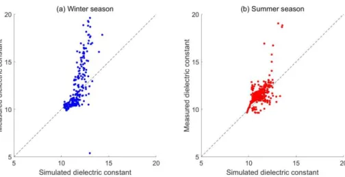
parameter values are then used in the subsequent SP simulations (Table 2). Figure 3 is
a scatter plot comparing the simulated and measured dielectric constant data for this
best-fitting model. The average absolute mean deviation is 0.7168. The simulated
dielectric constant underestimates the variability in the observed data, particularly
during the winter season when the water content can be very high due to decreased
evapotranspiration and snow melt events (Haarder et al., 2015).
Table 2: The parameter values of the maximum a posteriori model obtained by
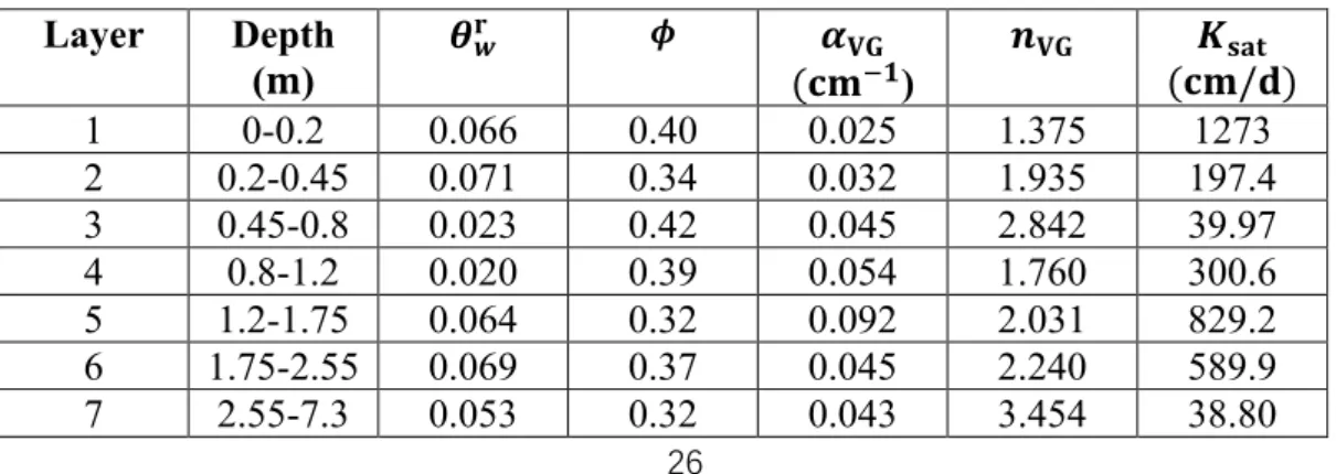
MCMC inversion. Layer Depth (𝐦) 𝜽𝒘𝐫 𝝓 𝜶 𝐕𝐆 (𝐜𝐦−𝟏) 𝒏𝐕𝐆 𝑲𝐬𝐚𝐭 (𝐜𝐦/𝐝) 1 0-0.2 0.066 0.40 0.025 1.375 1273 2 0.2-0.45 0.071 0.34 0.032 1.935 197.4 3 0.45-0.8 0.023 0.42 0.045 2.842 39.97 4 0.8-1.2 0.020 0.39 0.054 1.760 300.6 5 1.2-1.75 0.064 0.32 0.092 2.031 829.2 6 1.75-2.55 0.069 0.37 0.045 2.240 589.9 7 2.55-7.3 0.053 0.32 0.043 3.454 38.80
27
Fig. 3. Scatter plot of simulated dielectric constant against measured dielectric constant in the (a) winter season (October to March) and the (b) summer season (April to September) of 2012.
3.4. Self-potential data
With assuming only vertical flow, a total of 15 non-polarizable Petiau electrodes
(Pb/PbCl2, NaCl) were installed at depths of 0.25 m, 0.5 m, 0.75 m, 1 m, 1.45 m, 1.9 m,
3.1 m and 7.3 m in individual holes (Fig. 2c). Theses electrodes holes were drilled by
augering. Each electrode was inserted vertically in a thin hole and it was attached to a
wooden stick to ensure that the electrode had a good contact with the bottom of the hole
and to better estimate the depth of installation. The one exception to this procedure was
one of the top electrodes that was installed at 0.5 m in an individual dug hole, which
was later filled with bentonite. As shown in Fig. 2c, there are two electrodes installed
without bentonite surroundings at 0.25 m, 0.5 m, 0.75 m, 1 m and 1.45 m. The reference
electrode during the measurements was located well below the water table at 7.3 m
depth. To remove the strong influence of water table fluctuations from the acquired SP
28
depth) serve as the reference electrode. Due to the superposition principle, this is
achieved by subtracting the measured SP data at this location from all the other
measured SP time-series. Initially, from July 19, 2011 until September 9, 2011, SP data
were recorded every 20 minutes. Subsequently, SP data were recorded every 5 minutes.
Herein, we present data until July 28, 2015. Repeated crosshole ERT measurements
were performed in the area from September 2011 to August 2012 (Haarder et al., 2015),
leading to large recorded voltages that are unrelated to the processes of interest. To filter
out these effects, we first median filter the SP data at each recorded time 𝑡𝑖 within a
period of 𝑡𝑖− 75 minutes to 𝑡𝑖 + 75 minutes. Second, in the period of ERT
measurements we identify periods ∆𝑡𝑘 disturbed by the ERT measurements by
identifying times with anomalously high temporal SP variations. For these time-periods,
we replace the raw data with the median filtered data. Finally, we median filter the
resulting time-series using a 1-hour window corresponding to the time-interval used to
represent the SP data in this paper. See Mariethoz et al. (2015) for an alternative data
processing approach that has been demonstrated for a sub-set of the presented data.
4. Results
4.1. Calibration and sensitivity analysis of electrokinetic and electrochemical effects
We first consider the streaming potential generated by electrokinetic effects. In
doing so, we focus on the SP data acquired prior to the saline tracer injection. In this
29
and the electro-diffusive effect should be minimal. In addition to simulations using the
WR and RP methods mentioned in section 2.1.1, we also consider modeling based on
the thick double-layer assumption in which the effective excess charge density is scaled
with water saturation 𝜙
𝜃w (Linde et al., 2007a):
𝑄̂ (𝜃Lindeeff w, 𝐶w) = 𝜙
𝜃w𝑄
eff,sat
̂ (𝐶
w), (31)
where the saturated excess charge density 𝑄̂eff,sat(𝐶
w) is estimated by Eqs. (8) and (9).
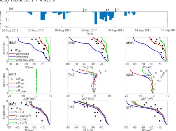
We present SP profiles (Figs. 4b-d) at three times corresponding to before, during and
after a rainfall event (Fig. 4a). As expected for a recharge-dominated regime with
associated downward flow, the recorded SP data (Figs. 4b-d) become increasingly
negative towards the surface. Furthermore, the electrodes located at the same depth
display similar SP values indicating that electrode-related effects are uniform. The
simulated SP signals have similar shapes (Figs. 4b-d), but it is only the WR method that
provides simulations of the same magnitude as the observed data. The RP method
overestimates the amplitudes roughly by a factor of two and the thick double-layer
assumption of Eq. (31) leads to simulated SP signals that are roughly 50% too small.
The temporal differences in the observed SP data (Figs. 4e-g) display small decreases
in SP magnitudes, which is in contrast to the simulations that show larger increases. In
the following, we only present predictions based on the WR method. In the simulations
described above, we used calibrated values of the inverse time constant 𝛾 = 0.025 d−1
30
signals. As shown in Figs. 4h-j, the vertical SP profiles are only slightly affected by the
delay factor for 𝛾 > 0.025 d−1.
Fig. 4. (a) Precipitation data with three chosen times (t1-t3) highlighted by black arrows. Comparison between observed and simulated SP profiles (b) before a heavy rain at t1, (c) during the rain at t2 and (d) after the rain at t3. The solid lines are simulated SP data using different excess charge densities 𝑄̂ obtained, respectively, from the WR method (red), the RP method (blue) and eff the thick double-layer model (green) of Linde et al. (2007). (e-g) Differences of observed SP (circles) and simulated SP (dashed lines) with respect to t1. (h-j) Simulated SP signals (solid lines) using the WR method with different γ-values in equation (26).
After choosing the WR method for calculating the effective charge density (Eq. 7)
and calibrating the delay factor at 𝛾 = 0.025 d−1 (Eq. 26) using the observed SP data
prior to saline injection, we now consider the SP simulations for longer time-series
including the saline tracer injection period. Following the ERT-based estimations of the
saline tracer test by Haarder et al. (2015), the dispersivity α (Eq. 25) is initially set to
31
to September 2012 at 0.25 m and 0.75 m (Fig. 5). The simulated SP data given as a
superposition of electrokinetic and electro-diffusive contributions without
electrode-related effects are presented in Figs. 5b and 5e. The simulated SP signals describe the
main shape of the observed SP data rather well, particularly the strong response caused
by the saline tracer injection. To assess electrode-related effects, we first consider the
estimated macroscopic Hittorf number 𝑇Na∗ of the electrode clay-mixture calculated by
Eq. (20). The simulated SP signals including the electrode-effect (Figs. 5c and 5f)
display a much slower decrease in SP amplitudes after the tracer injection than what is
observed, and the gradual relaxation observed in the data towards more negative values
is not reproduced. We then sought the macroscopic Hittorf number 𝑇Na∗ that maximises
the correlation between the observed and simulated SP data. In Figs. 5d and 5g, we
display the prediction for the best-fitting calibrated value of 0.43. This higher value is
rather consistent with the fact that the clay allows a larger mobility of the cation due to
an important volume of EDL in its pore space (see discussion in Revil and Jougnot,
2008). Here, the simulated responses are found to be intermediate between the two other
cases. For the shallow electrode, we see that the decrease of SP magnitudes (Fig. 5d)
32
in better agreement with the observed data.
Fig.5. (a) Precipitation data during the first year of SP monitoring with the red arrow indicating the time of saline tracer injection. Solid black and dashed lines indicate the observed SP data at two measuring electrodes located at (b-d) 0.25 m and (e-g) 0.75 m depth. (b, e) The sum of the simulated streaming potential and electro-diffusive potential is shown in blue. The sum of the simulated streaming potential, electro-diffusive potential and electrode membrane potential with (c, f) the calculated macroscopic Hittorf number of the electrode clay mixture in purple and (d, g) with the best fitting macroscopic Hittorf number (0.43) in red.
Using the optimized 𝑇Na∗ = 0.43 for the electrode clay mixture, we now investigate
the sensitivity of our simulated SP responses to the dispersivity α. The impact of α at
33
magnitudes decrease following the tracer injection, with faster decreases observed for
larger α, and the rate of relaxation towards more negative values being the strongest for
small α. The most satisfactory simulations are offered by α = 0.1 m and this value is
retained in the following. As an aside, we note that the observed SP curves at 0.25 m
(Fig. 6a) present a notable decrease in February 2012, which is attributed to the partially
frozen topsoil (and electrode). Indeed, the soil temperature at this depth is below 0 ℃
in this time period.
In Fig. 7, we present the simulated spatio-temporal evolution of the solute
concentration, which suggests that all of the injected saline should have reached the
groundwater in April 2013. The trajectory of the simulated maximum concentration
agrees well with the ERT-based estimates (Haarder et al., 2015), with both showing an
acceleration of the plume movement in the winter. We note further that our estimates
are in-between the ERT-based estimates of Haarder et al. (2015) and those determined
34
Fig. 6. Comparison between the observed (black solid and dashed lines) and simulated SP signals using the best fitting macroscopic Hittorf number (0.43) for different values of dispersivity at (a) 0.25 m and (b) 0.75 m depth. The chosen values of dispersivity are 0.05 m (green), 0.1 m (purple), 0.15 m (blue) and 0.25 m (red). The red arrow indicates the time of saline tracer injection and the blue arrows indicate the frozen period.
35
Fig. 7. The spatio-temporal variations of the simulated solute concentration of pore water assuming a dispersivity of 0.1 m. The dashed line corresponds to the depth of maximum concentration, the black triangles indicate the center of solute mass determined by drilled core data and the red diamonds are the center of solute mass inferred by Haarder et al. (2015) using ERT data.
4.2. Electrode stability
Using the calibrated parameters, we simulate the SP responses as a superposition of
electrokinetic, electro-diffusive, and electrode-related effects over four years and
consider five vertical SP profiles in the summer seasons of 2011, 2012, 2013, 2014, and
2015 (Fig. 8). The corresponding dates were chosen to correspond to periods with heavy
rainfall implying that the simulated SP data have similar shapes and magnitudes at all
of the considered dates. However, it is only in 2011 (Fig. 8a) shortly after the SP
installations that the observed SP data also show a trend of increasingly negative values
towards the surface as expected for an infiltration-dominated system. At later years, the
observed data start to deviate from this expected behavior. The observed data are
36
oscillations with depth. This pattern is similar in 2013 (Fig. 8c), but with smaller
magnitudes. The observed SP data turn positive in 2014 (Fig. 8d) and the magnitudes
of the most positive values in 2015 approach 200 mV (Fig. 8e), thus, the different scale
used on x-axis of Fig. 8e. Since no major changes in the state of the vadose zone is
expected between these years as indicated by the simulated data, this suggests that the
observed differences between the years are largely due to time-varying electrode
polarizations manifesting themselves by electrode-potentials that develop differently
with depth (different water content magnitudes and dynamics).
Fig. 8. Comparison between observed (black dots) and simulated (red lines) SP profiles on (a) 07 September 2011, (b) 22 August 2012, (c) 10 August 2013, (d) 30 August 2014 and (e) 28 July 2015 (e), respectively. These dates in during the late summer period of each year were chosen to correspond to days just during important rain events (25.32 mm, 33.77 mm, 18.66 mm, 22.48 mm and 37.74 mm, respectively).
4.3. SP responses to infiltration events after years of monitoring
Based on the simulation of solute transport presented in Fig. 7, the injected saline
water should disappear from the vadose zone after April 2013. Figure 8 highlighted
37
that we are unable to explain without invoking changes in the electrode potential (i.e.,
electrode drifts). The common approach when facing unexplained electrode offsets, is
to refer to changes in the SP data with respect to a reference datum. This approach can
only work satisfactorily if the “electrode drift” is slow and unrelated to the local water
content and salinity. With the aim of highlighting the SP response to heavy rainfall
events after more than three years of monitoring, we consider the SP data at 0.25 m and
1.9 m during three days in the summer of 2014 and the winter of 2015, respectively. We
show the curves in Figs. 9 and 10 with different scales, as there are large differences in
amplitudes between 0.25 m and 1.9 m. In Figs. 9 and 10, the SP data are presented as
relative changes compared with the SP data recorded at the corresponding depth at
00:00:00 on August 30, 2014 and at 12:00:00 on January 7, 2015, respectively. This
type of re-referencing of SP data is very common (e.g., Linde et al., 2007a).
Furthermore, the reference electrode was set at 2.5 m to focus on temporal changes in
the near surface. The periods were chosen to correspond to a long dry period followed
by heavy rainfall (Fig. 9a and Fig. 10a) leading to strong changes in water content (Figs.
9b, d and Figs. 10b, d). In the summer season of 2014, one of the SP electrodes at 0.25
m show responses corresponding to the timing of changes in the water content. At 1.9
m, there is an SP response (Fig. 9e) with the same sign as in the winter (Fig. 10e), but
the initiation of the SP signal occurs with a time delay with respect to the water content
signal (Fig. 9d). Considering the winter period, the SP data at 0.25 m (Fig. 10c) do not
show a clear unambiguous relationship to the rainfall event and the two SP electrodes
38
increasing negative amplitudes starting at a time that is only slightly earlier than the
response in the water content at 2.0 m (Fig. 10d). These differences might suggest
significant lateral variations in vertical flow.
Fig. 9. SP responses observed during a period with significant rain events separated by dry periods in the summer of 2014. (a) Precipitation data; (b) measured water content data at 0.25 m; (c) observed SP data at 0.25 m; (d) measured water content data at 2 m and (e) observed SP data at 1.9 m. Here, the SP reference is located at 2.5 m depth and the amplitudes are set to zero at the beginning of the plotted period.
39
Fig. 10. SP responses observed during a period with significant rain events separated by dry periods in the winter of 2015. (a) Precipitation data; (b) measured water content data at 0.25 m; (c) observed SP data at 0.25 m; (d) measured water content data at 2 m and (e) observed SP data at 1.9 m. Here, the SP reference is located at 2.5 m depth and the amplitudes are set to zero at the beginning of the plotted period.
5. Discussion
5.1. SP-data with bentonite installation
The electrode surrounded by bentonite was installed several meters away from the
saline injection area and is likely unaffected by the saline injection. The bentonite with
its low permeability is likely to offer a stable environment in which water content and
salinity variations are low. Indeed, the use of bentonite is often recommended for SP
monitoring (Petiau, 2000). We consider here the SP data at 0.5 m, from the installation
40
signals are of electrokinetic origin. The overall shape of the SP electrode in bentonite
(Fig. 11b) is similar to the numerical simulations, which ignores the presence of the
bentonite (Fig. 11d). The two time-series show a stepped shape with declines occurring
around July 22, August 7 and September 6 corresponding to the main rain events in this
time-period. On top of this, the electrode in the bentonite shows a shift in magnitude
and a linear drift with increasing negative values over time that is not present in the
simulated data. One of the electrodes installed at 0.5 m (Fig. 11c) shows temporal
variations corresponding to the same events, but the magnitudes are smaller than in the
bentonite and the polarity of the response is not always the same (negative on July 22,
negative on August 7 and positive on September 6).
Fig. 11. (a) Precipitation data in the considered time period. Comparison between the observed SP signals in (b) bentonite with (c) observed SP signals without bentonite installation and (d) simulated SP ignoring the presence of the bentonite at 0.5 m. SP data were not recorded from 26 August 2011 to 30 August 2011.
A notable feature is clearly that the SP signals in the bentonite (Fig. 11b) are much
smaller (-65 mV on average) than the other SP electrodes at the same depth (Fig. 11c)
and the simulated SP data (Fig. 11d). This is likely related to the fact that bentonite is a
41
electric double layers (EDL). One would thus expect anion exclusion effects (Jougnot
et al., 2009; Leinov and Jackson, 2014) implying that Cl− is excluded from the pore
space, leading to a different macroscopic Hittorf number 𝑇Naben in the bentonite
compared to the surrounding. Considering the simple case for which the soil salinity is
uniform, the difference of SP between the bentonite 𝑆𝑃benexc and the surrounding soil
𝑆𝑃soilele is:
∆𝜑benexc = 𝑆𝑃benexc− 𝑆𝑃soilele
= −kB𝑇K e0 (2𝑇Na ∗ − 1)ln 𝐶ele 𝐶ben− kB𝑇K e0 (2𝑇Na ben− 1)ln𝐶ben 𝐶soil +kB𝑇K e0 (2𝑇Na ∗ − 1)ln𝐶ele 𝐶soil = kB𝑇K e0 (1 − 2𝑇Na ∗ )ln𝐶soil 𝐶ben+ kB𝑇K e0 (1 − 2𝑇Na ben)ln𝐶ben 𝐶soil (32)
where 𝐶ele , 𝐶ben and 𝐶soil are the ion concentrations inside the electrode, in the
bentonite and in the surrounding soil. Considering the limiting case 𝑇Naben = 1, ∆𝜑 benexc
could be -66.32 mV when 𝐶ben
𝐶soil = 10 and 𝑇Na
∗ = 0.43 at 20℃ (293.15 K) in good
agreement with the observations in Figs. 11b and 11c. This example suggests that the
electrode installation method has a large effect on the measured SP signals (absolute
amplitudes, drifts and sensitivity to perturbations) and that monitoring of ion
concentrations or suitable proxies (e.g., electrical conductivity) in the vicinity of the
42
5.2. Electrode effects
One risk in the context of multi-year SP monitoring is that other ions than Cl− that
are naturally present in the soil enter into contact with the lead wire through diffusion
(Petiau, 2000). This may lead to unpredictable perturbations of the electrode
polarization that arise well before the desaturation time of Cl− (Petiau, 2000). Judging
from our data (Fig. 8), an even larger risk is related to dehydration of the electrolyte by
capillarity occurring when the SP electrodes are installed under unsaturated conditions
with the dehydration process varying over time and space as the capillary pressure
varies. In contrast to the short-term laboratory findings by Petiau (2000) discussed in
section 2.1.3, our long-term field-based results suggest that the lifespan of Petiau
electrodes is greatly reduced in partially saturated media. We attribute this to capillary
suction removing the electrolyte from the clay mud inside the electrodes. Petiau (2000)
reports that the measured electrode potential increases when the electrodes dry out as a
consequence of the limited contact between the remaining electrolyte and the lead wire
inside the electrodes. This is in strong agreement with the observed shift towards
positive values over time (Fig. 8). Our field observations suggest that Petiau electrodes
installed in the vadose zone have considerably shorter life-times than previously
suggested by Petiau (2000).
It could be argued that the impact of time-varying saturation and concentration state
on the electrodes could be included in the modeling and that their impact on the
measured SP data could be predicted. However, observed differences between
43
when considering 1-D flow and transport simulations. To characterize this aspect of
electrode drift related to local variations in the electrode installation, geological
heterogeneity and perhaps the electrodes themselves, we plot the median of the absolute
deviation of the electrode pairs installed at common depths (Fig. 12a). The electrodes
are stable with low absolute deviations before May 2012, after which the discrepancies
increase and reach a peak of almost 40 mV around May 2013. It is also seen that the
median of the absolute deviations is overall lower in the summers than in the winters.
The largest absolute deviations are found for the shallow electrodes. This behavior is
also seen in Fig. 5, in which the deviations among the electrode pairs increase notably
after May 2012. The median value of the absolute deviation between simulated water
content and measured water content inverted by measured dielectric constant data using
Eq. (27) shows similar seasonal trends (Fig. 12b). Figure 12b offers, thus, some possible
insights regarding the possible causes of the larger absolute deviations in the observed
SP data (Fig. 12a) during the winter period. Indeed, partial freezing of the soil and snow
accumulation on the surface lead to heterogeneous melt water infiltration (making the
underlying 1-D assumption increasingly questionable) and various measurement issues
44
Fig. 12. (a) Temporal variation of the absolute median deviation of observed SP data at depths (0.25 m, 0.5 m, 0.75 m, 1 m, 1.45 m) with two measurement electrodes. The corresponding absolute median deviations of each electrode pair for the whole time period are 15.08 mV, 12.92 mV, 9.03 mV, 9.04 mV, 8.96 mV, respectively. (b) Temporal variation of the absolute median deviation of observed water content data with simulated water content data at depths (0.25 m, 1 m, 1.5 m, 2 m, 2.25 m, 2.5 m, 2.75 m, 3 m). The corresponding absolute median deviations at each depth over time are 0.03, 0.02, 0.03, 0.01, 0.02, 0.02, 0.02, 0.02, respectively.
6. Concluding remarks
The analysis of four years of SP monitoring data at the HOBE hydrological
45
vadose zone is still a largely unresolved challenge. The main complication is the strong
variability of the effective excess charge ( 𝑄̂ (𝜃eff
w, 𝐶w) ) and the difficulties in
predicting this function accurately. Traditionally, it is expected that streaming potential
magnitudes increase when water fluxes increase (e.g., Doussan et al., 2002). However,
this does not need to be the case and increased flow might actually lead to decreases in
the observed SP amplitudes (see Figs. 4f and 4g). As the water content increases,
𝑄̂ (𝜃eff w, 𝐶w) decreases particularly at the onset of fluid flow in macro pores (these
pores carry a lot of flow without a significant drag of excess charge). So, this decrease
in 𝑄̂ (𝜃eff
w, 𝐶w) might offset the increase in current density offered by the increasing
water flux u (Eq. 5), while the increasing water content increases electrical conductivity
(Eq. 3), thereby, decreasing the observed self-potential (Eq. 2). Calibration of such
non-linear functions as 𝑄̂ (𝜃eff
w, 𝐶w) to achieve high predictive capability is very
challenging. Dual-domain formulations of porosity need to be considered to account
for the influence of macro pores on flow, transport and electrical properties (see also
discussion Romero-Ruiz et al. 2019). This work has also highlighted the need to
accurately model the time-evolving water salinity, which implies that water-soil
interactions need to be accounted for, and that water salinity needs to be monitored.
Furthermore, it is probably also needed to account for the fact that flux-averaged soil
water concentrations are different from in-situ concentrations (e.g., Evaristo et al.,
2015). This implies that predictive SP modeling in the vadose zone does not only need
to consider advanced SP theory, but also state-of-the-art flow and transport modeling
46
work clearly highlights that SP signals in the vadose zone cannot be interpreted as a
sensor of water movement by simply differencing SP differences between neighboring
depth levels. The reality is much more complicated than this even in absence of
electrode effects.
Our study confirms suggestions by Perrier et al. (1997) and Doussan et al. (2002)
that the design and installation of SP-electrodes for long-term monitoring in the vadose
zone is a largely open topic. Important electrode-related challenges in predictive SP
modeling concern (i) the membrane polarization between the interior of the electrode
and its immediate surroundings and (ii) dehydration of the electrodes by capillary forces
impacting electrode potentials. Except for one electrode, we did not follow the common
approach of installing the electrodes in a bentonite solution (Perrier et al., 1997; Petiau,
2000; Doussan et al., 2002). Clearly, a bentonite solution improves the contact
resistance with the ground and makes the data less sensitive to small-scale
heterogeneity (Petiau, 2000). However, it also leads to difficult-to-predict
electro-diffusive effects as the bentonite equilibrates with the surrounding media and the
electrode solution leading in our case to large electrode offsets with respect to other
electrodes and enhanced drifts (Fig. 11b). For instance, the soil mud in which Doussan
et al. (2002) inserted their electrodes displayed a threefold decrease in the pore water
electrical conductivity during the monitoring period and, thus, a similar decrease in
salinity. This implies significant electro-diffusive effects of 3-D nature in the soil and
does not ensure constant water salinity at the contact with the electrode. For future
47
monitored, which would help to elucidate some of the behaviors that we report.
Acknowledgments
We thank the Danish hydrological observatory HOBE for providing access to the
site, technical help, and full access to the data. The data used in this paper are available
here: http://dx.doi.org/10.17632/6r8898657w.1. To calculate the SP signals, we used a
version of Maflot (maflot.com) that was kindly provided by I. Lunati and R. Künze and
modified by M. Rosas-Carbajal. We are grateful for the financial support offered by the
China Scholarship Council and the helpful reviews by Emily Voytek and André Revil.
References
Andreasen, M., Jensen, K. H., Desilets, D., Zreda, M., Bogena, H., Loom, M. C., 2017. Cosmic-ray neutron transport at a forest field site: the sensitivity to various environmental conditions with focus on biomass and canopy interception. Hydrol. Earth Syst. Sci. 21, 1875-1894.
https://doi.org/10.5194/hess-21-1875-2017.
Andreasen, M., Jensen, K. H., Zreda, M., Desilets, D., Bogena, H., Loom, M. C., 2016. Modeling cosmic ray neutron field measurements. Water Resour. Res. 52, 6451-6471.
https://doi.org/10.1002/2015WR018236.
Archie, G., 1942. The electrical resistivity log as an aid in determining some reservoir characteristics. Trans. Am. Inst. Min. Metall. Eng. 146, 54-61. https://doi.org/10.2118/942054-G.
Bear, J., 2012. Hydraulics of groundwater. Courier Corporation.
Castermant, J., Mendonça, C. A., Revil, A., Trolard, F., Bourrié, G., Linde, N., 2008. Redox potential distribution inferred from self-potential measurements associated with the corrosion of a burden