The Molecular Gas Content and Fuel Efficiency of Starbursts at z ∼ 1.6 with ALMA

HAL Id: hal-02043173

https://hal.archives-ouvertes.fr/hal-02043173

Submitted on 21 Jan 2020

HAL is a multi-disciplinary open access

archive for the deposit and dissemination of

sci-entific research documents, whether they are

pub-lished or not. The documents may come from

teaching and research institutions in France or

abroad, or from public or private research centers.

L’archive ouverte pluridisciplinaire HAL, est

destinée au dépôt et à la diffusion de documents

scientifiques de niveau recherche, publiés ou non,

émanant des établissements d’enseignement et de

recherche français ou étrangers, des laboratoires

publics ou privés.

The Molecular Gas Content and Fuel Efficiency of

Starbursts at z

∼ 1.6 with ALMA

J. D. Silverman, W. Rujopakarn, Emanuele Daddi, A. Renzini, G. Rodighiero,

D. Liu, A. Puglisi, M. Sargent, C. Mancini, J. Kartaltepe, et al.

To cite this version:

J. D. Silverman, W. Rujopakarn, Emanuele Daddi, A. Renzini, G. Rodighiero, et al.. The Molecular

Gas Content and Fuel Efficiency of Starbursts at z

_{∼ 1.6 with ALMA. The Astrophysical journal}

The Molecular Gas Content and Fuel Ef

ficiency of Starbursts at z∼1.6 with ALMA

C. Mancini6,5 , J. Kartaltepe8 , D. Kashino9 , A. Koekemoer10 , N. Arimoto11,12, M. Béthermin13 , S. Jin4,14, G. Magdis15 , T. Nagao16 , M. Onodera12 , D. Sanders17 , and F. Valentino18

1

Kavli Institute for the Physics and Mathematics of the Universe, The University of Tokyo, Kashiwa, 277-8583(Kavli IPMU, WPI), Japan;silverman@ipmu.jp

2

Department of Physics, Faculty of Science, Chulalongkorn University, 254 Phayathai Road, Pathumwan, Bangkok 10330, Thailand 3

National Astronomical Research Institute of Thailand(Public Organization), Don Kaeo, Mae Rim, Chiang Mai 50180, Thailand 4_{Laboratoire AIM, CEA/DSM-CNRS-Universite Paris Diderot, Irfu/Service d’Astrophysique, CEA Saclay, France}

5

INAF—Osservatorio Astronomico di Padova, Vicolo dell’Osservatorio 5, I-35122, Padova, Italy 6

Dipartimento di Fisica e Astronomia, Universita di Padova, vicolo Osservatorio, 3, I-35122, Padova, Italy 7

Astronomy Centre, Department of Physics and Astronomy, University of Sussex, Brighton, BN1 9QH, UK 8

School of Physics and Astronomy, Rochester Institute of Technology, 84 Lomb Memorial Drive, Rochester, NY 14623, USA 9

Department of Physics, ETH Zürich, Wolfgang-Pauli-Strasse 27, CH-8093, Zürich, Switzerland 10

Space Telescope Science Institute, 3700 San Martin Drive, Baltimore, MD 21218, USA 11

Astronomy Program, Department of Physics and Astronomy, Seoul National University, 599 Gwanak-ro, Gwanak-gu, Seoul, 151-742, Republic of Korea 12

Subaru Telescope, 650 North A’ohoku Place, Hilo, HI 96720, USA 13

Aix Marseille Université, CNRS, LAM(Laboratoire d’Astrophysique de Marseille) UMR 7326, F-13388 Marseille, France 14

Key Laboratory of Modern Astronomy and Astrophysics in Ministry of Education, School of Astronomy and Space Sciences, Nanjing University, Nanjing, 210093, People’s Republic of China

15

Cosmic DAWN Centre, Niels Bohr Institute, University of Copenhagen, Juliane Mariesvej 30, DK-2100, Copenhagen, Denmark 16

Research Center for Space and Cosmic Evolution, Ehime University, 2-5 Bunkyo-cho, Matsuyama 790-8577, Japan 17

Institute for Astronomy, University of Hawaii, 2680 Woodlawn Drive, Honolulu, HI 96822, USA 18

Dark Cosmology Centre, Niels Bohr Institute, University of Copenhagen, Juliane Maries Vej 30, DK-2100 Copenhagen, Denmark Received 2018 May 15; revised 2018 August 24; accepted 2018 September 14; published 2018 November 2

Abstract

We present an analysis of the molecular gas properties, based on CO(2−1) emission, of 12 starburst galaxies at z∼1.6 selected by having a boost (4×) in their star formation rate (SFR) above the average star-forming galaxy at an equivalent stellar mass. ALMA observations are acquired of six more galaxies than previously reported through our effort. As a result of the larger statistical sample, we significantly detect, for the first time at high z, a systematically lowerLCO¢ /LIRratio in galaxies lying above the star-forming“main sequence” (MS). Based on an

estimate ofαCO(i.e., the ratio of molecular gas mass to ¢LCO 1 0- ), we convert the observational quantities (e.g., ¢

LCO/LIR) to physical units (Mgas/SFR) that represent the gas depletion time or its inverse, the star formation

efficiency. We interpret the results as indicative of the star formation efficiency increasing in a continuous fashion from the MS to the starburst regime, whereas the gas fractions remain comparable to those of MS galaxies. However, the balance between an increase in star formation efficiency and gas fraction depends on the adopted value of αCOas discussed.

Key words: galaxies: high-redshift– galaxies: ISM – galaxies: starburst – galaxies: star formation

1. Introduction

On occasion, galaxies experience a rapid rise in their production rate of forming new stars, usually referred to as a starburst (e.g., Sanders & Mirabel 1996). Such explosive

phenomena, in the local universe, are the result of the merger of two massive, gas-rich galaxies that induce intense star formation and can boost the growth of their central supermassive black hole (e.g., Di Matteo et al. 2005; Hopkins et al. 2006; Volonteri et al.2015). It remains to be demonstrated whether the

same process is also responsible for starburst galaxies in the early universe, with star formation rates (SFRs) several times higher than those of more common galaxies. Recent hydro-dynamical simulations of galaxy mergers(Fensch et al.2017) at

high redshifts show rather mild boosts in star formation, as compared to the typical star-forming galaxy population, which is attributed to the already-enhanced SFRs as a result of their high gas fractions. While such starburst galaxies do not appear to be the leading mechanism responsible for the cosmic history of star formation(Lotz et al.2008; Rodighiero et al.2011; Sargent et al.

2012; Lackner et al. 2014), they may still represent a crucial

passage in the life cycle of galaxies.

Local starbursts appear to support the scenario of having a higher efficiency in forming stars (Solomon et al. 1997) and

suggest a different mode of star formation distinct from that of typical star-forming galaxies (Daddi et al. 2010b; Genzel et al. 2010). However, it is still unclear whether starbursts,

including those at higher redshifts, are the result of either enhanced levels of molecular gas out of which stars form(i.e., a higher gas fraction; Scoville et al. 2016; Lee et al. 2017), a

higher efficiency to form stars from a given supply of gas (Magdis et al. 2012a; Genzel et al. 2015; Silverman et al.

2015a; Elbaz et al.2018), or a combination of both (Combes

et al. 2013; Scoville et al. 2017; Tacconi et al. 2017). It

is therefore imperative to establish whether such different modes of star formation are active at earlier stages in the evolution of our universe when most of the star formation was actually taking place. Alternatively, the efficiency to form stars may be a continuous function with distance above the star-forming “main sequence” (MS; Speagle et al. 2014; Renzini & Peng2015). With sufficient investigations, we can

also determine whether mergers are the sole mechanism responsible for enhanced star formation efficiency (SFE) or whether other processes, such as violent disk instabilities

(Bournaud et al.2010; Dekel & Burkert2014), can drive SFRs

well above that of the typical star-forming MS. Carilli & Walter (2013) present a overview of the molecular gas properties of

high-redshift star-forming galaxies as related to this topic. To address these issues, we have undertaken a study, asfirst presented in Silverman et al.(2015a), to measure the molecular

gas properties using carbon monoxide 12CO, primarily the J=2−1 transition, of galaxies in the COSMOS field (Scoville et al. 2007) having SFRs well above (4×) the star-forming

MS at z∼1.6. Observations are mainly acquired with the Atacama Large Millimeter/submillimeter Array (ALMA) and supplemented with those from the Northern Extended Milli-meter Array (NOEMA) Interferometer. The rotational trans-ition CO (2−1) is at an excitation level close to the locally calibrated tracer CO (1−0) of the total molecular gas mass; thus, it has been used for many studies of high-redshift galaxies to date(e.g., Tacconi et al.2017).

Our starburst sample has been selected to span a narrow range of accurate spectroscopic redshifts(z∼1.6) from which it has been drawn(Silverman et al.2015b). At these redshifts,

there are still limited numbers of starburst galaxies with CO observations in the literature (see Figure2 of Tacconi et al.

2017). The stellar mass and SFRs of galaxies in our sample are

based on mid- and far-IR observations from the Spitzer and Herschel satellites, placing them securely in the starburst class (Rodighiero et al. 2011) and matching fairly well in stellar

mass to existing samples of more normal galaxies with CO detections at a similar redshift. Being located in the COSMOS field, we have a wealth of multiwavelength data across the electromagnetic spectrum; thus, our approach, in particular the selection method, complements that used in the literature for starburst galaxies, such as the brightest submillimeter galaxies (SMGs) at high z (e.g., Ivison et al. 2005, 2011; Casey et al.2011,2017; Danielson et al.2017). Compared to classical

SMGs, our selection avoids contamination by massive galaxies on the MS(Magnelli et al.2012), reduces SED bias compared

to SMG selection (which prefers cold objects), and is able to pick objects even with less extreme SFRs, but much higher above the MS population. We refer the reader to Casey et al. (2014), which provides a comprehensive review of the vast

literature on dust-obscured star-forming galaxies at high redshift.

To build on our past study, we report here on ALMA observations of the molecular gas content as traced by CO (2−1) of six additional starburst galaxies that have SFRs highly elevated (4×) from the star-forming MS at z∼1.6. This larger sample of 12 galaxies enables us to confirm trends (e.g., ¢LCO/á ¢ ñLCO MSvs. dMS= sSFR/ásSFRñMS, where sSFR=SFR/Mstellar) seen in the previous study with

higher statistical significance due to the larger size of the sample and higher boost in SFR above the star-forming MS. We present our results with consideration of the likely range of the factor (αCO) required to convert CO luminosity to

molecular gas mass(Bolatto et al.2013; Carleton et al.2017),

a critical aspect of this analysis. Correspondingly, we have measuredαCObased on dynamical arguments for three

of our sources, as presented in Silverman et al. (2015a)

and Silverman et al. (2018), and have information on the

metallicity from the [NII]/Hα ratio acquired through near-infrared spectroscopy(Zahid et al.2014; Kashino et al.2017; Puglisi et al. 2017). Throughout this work, we refer to the

total molecular gas mass as primarily composed of H2 and

He, and we assume H0=70 km s−1Mpc−1, ΩΛ=0.7, and

ΩM=0.3. We use stellar masses and SFRs converted to a

scale based on a Chabrier initial mass function (IMF); we chose this IMF (different from that presented in Silverman et al.2015a) to aid in comparisons with the literature (Sargent

et al.2014; Tacconi et al.2017).

2. Selection of the Sample and Physical Characteristics To construct a robust sample of starburst galaxies at z∼1.6, we first acquired spectroscopic redshifts of Herschel sources through the FMOS-COSMOS survey(Silverman et al.2015b),

a spectroscopic survey of star-forming galaxies at 1.4 z1.7 in the near-infrared (1.11–1.35 μm and 1.6–1.8 μm) using the instrument FMOS(Kimura et al.2010) on the Subaru

Telescope. Fibers were allocated to Herschel sources with a high priority, especially for those having SFRs that place them above (>4×) the MS (see below). Spectroscopic redshifts are determined from the centroid of the Hα emission line with additional lines ([NII] λ6584, [OIII] λ5008, and Hβ), providing further assurance of the redshift. These emission lines also provide a measure of the level of dust extinction and chemical enrichment. On the rest-frame optical emission line properties of high-z starbursts, we refer to a separate study (Puglisi et al. 2017) that makes use of a larger sample than

presented here since only a subset of the outliers from the MS have been observed with ALMA. In Figure1, we present the SFR and stellar mass distribution of the full sample of 108 galaxies detected by Herschel and having spectroscopic redshifts(1.4<z<1.7) from our FMOS-COSMOS program.

2.1. Stellar Mass

Stellar masses are determined byfitting the spectral energy distribution (SED) using Hyperz (Bolzonella et al. 2000) and

stellar population synthesis models(Bruzual & Charlot2003),

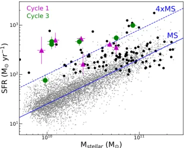
Figure 1. SFR vs. Mstellar for star-forming galaxies (including starbursts

detected by Herschel) at 1.4<z<1.7. The large colored symbols indicate the 12 starbursts observed by ALMA(Cycle 1: magenta; Cycle 3: green) that constitute the focus of our study. With black symbols, we indicate the location of Herschel-detected galaxies that have spectroscopic redshifts over the same interval from the FMOS-COSMOS survey. Smaller circles show the location of MS galaxies(gray) having photometric redshifts from Laigle et al. (2016). The

solid line indicates the MS, as determined by afit to the gray data points having sSFR>2×10−10yr−1, and a parallel track(dashed) at an elevated rate of 4×above the MS that illustrates the typical boosts in SFR for our starbursts.

based on a Chabrier IMF, at the FMOS spectroscopic redshift. Our motivation to recompute the stellar masses ourselves, for the initial selection, was to have consistency for both starbursts and MS galaxies as done in Puglisi et al. (2017). This ensures

that the enhancement in SFR for the starbursts, at a given stellar mass, is not due to different methods applied to each galaxy type. We implement constant star formation histories while being aware that the stellar masses may be systematically lower than if assuming an exponentially declining model with a recent burst of star formation. Photometric data cover the full spectrum from the near-UV to the IR, with the latter being especially important for stellar mass estimates of our highly

obscured starbursts. The COSMOS field has deep imaging

from UltraVISTA (YJHKS; McCracken et al. 2012), Subaru

Hyper Suprime-Cam(grizy; Tanaka et al.2017), and Spitzer/

IRAC(3.6, 4.5, 5.8, and 8.0 μm; Sanders et al.2007; P. Capak et al. 2018 in preparation). Spitzer MIPS 24 μm priors are used for deblending Herschel(or 70 μm Spitzer) sources required for accurate estimate of SFR. The stellar masses are in very good agreement with those given in Laigle et al. (2016) while

considering differences between the spectroscopic and photo-metric redshifts.

2.2. SFR

For all Herschel-detected starbursts with spectroscopic redshifts, SFRs are determined from the total infrared (TIR) luminosity LTIR and the calibration of Kennicutt & Evans

(2012) to fully account for the obscured component that

dominates the emission from starbursts (∼90%; Rodighiero et al. 2011). We use the long-wavelength photometry from

Spitzer(24 μm; Sanders et al.2007), Herschel PACS (100 and

160μm; Lutz et al.2011), and SPIRE (250, 350, and 500 μm)

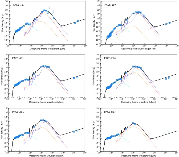
bands, available over the COSMOSfield. In Figure2, we show the SEDs of our starbursts(observed with ALMA in Cycle 3). The photometric data are fit with a dust model (Draine & Li

2007), with the integral from 8 to 1000 μm providing our

measure of LTIR.

A galaxy is defined to be a starburst if the SFR exceeds, at their respective stellar mass, the mean SFR of MS galaxies by a factor4 (Figure1). This is effectively a selection in sSFR and

not a cut on SFR alone. Our starburst sample, observed with

ALMA, has SFRs ranging from ∼100 to 1000 M_eyr−1

(Table 1). As a confirmation on the accuracy of the SFRs,

the radio emission, as detected by the VLA at 1.4(Schinnerer et al. 2007) and 5 GHz (Smolčić et al.2017), is in very good

agreement with the power-law synchrotron component as shown in each panel of Figure2that has a normalization only set by the infrared—radio relation. In Figure1, the distribution of star-forming galaxies in theSFR- Mstellar plane illustrates the robust selection of outliers (i.e., starbursts) that fall above the star-forming MS as indicated by the best-fit linear relation (Equation (1)) to 5266 sBzK-selected galaxies (Daddi

et al. 2004; Puglisi et al. 2017) in the COSMOS field with

1.4<zphot<1.7.

=  ´ M -  ( )

log SFR 0.91 0.09 log stellar 7.70 0.10. 1

By selecting galaxies based on their sSFR(Rodighiero et al.

2011), we avoid the inclusion of star-forming galaxies at the

massive end of the MS that would be selected if employing a method (e.g., submillimeter flux alone) primarily sensitive to SFR. This requires an accurate determination of the

star-forming MS that has been achieved with our FMOS-COSMOS sample(Kashino et al. 2013). For this purpose, we

rely on accurate measurements of stellar mass and SFRs provided by the COSMOS multiwavelength effort, particularly the deep IR imaging with UltraVISTA and Herschel photo-metry as described above. This method allows us to select objects offset(4× above) from the MS but less extreme than ULIRGs at low redshift.

2.3. Cycle 1 ALMA Sample

The five Herschel-detected starbursts observed in Cycle 1 with ALMA, as fully described in Silverman et al. (2015a),

were selected to have a boost in SFR greater than 4×above the MS at their respective stellar mass, while the Cycle 3 observations, presented below, are selected to be further elevated from the MS. The Cycle 1 sample has spectroscopic redshifts within 1.44<zspec<1.66, stellar masses between

1010 and 1011M_e, and SFRs greater than 300 M_eyr−1, with the exception of one of them (PACS-325) at a slightly lower SFR(Table 1).

Total CO(2−1) emission was detected for five galaxies with aflux density for each ranging between 0.37 and 2.7 mJy and at a significance greater than 4.7σ. Having been observed at higher spatial resolution (beam size of 1 3×1 0), two sources (PACS-819 and PACS-830) show signs of extended emission, while the rest are unresolved. The size and velocity measurements for these two enable us to estimate their gas mass, independent of CO luminosity, through dynamical arguments, thus making an estimate of the conversion factor αCO, the ratio of molecular gas mass to CO(1−0) luminosity.

Further details on the scientific results are given in Silverman et al. (2015a). For the remainder of this investigation, we

extend the analysis to 12 starbursts, with 11 based on ALMA observations and a single observation of PACS-164(Silverman et al.2015a) with the NOEMA interferometer. We chose not to

include the CO (3−2) observation of PACS-282 since the galaxy is at a higher redshift (z=2.187) than the rest of the sample.

2.4. Comparison Sample

For subsequent comparative analyses, a reference sample is utilized as compiled by Sargent et al.(2014) that includes 131

“typical” star-forming galaxies at z4 with measurements of their CO luminosity(Figure3). Here, we list and give credit to

the teams responsible for these data sets. In the local universe, the HERACLES survey(e.g., Leroy et al. 2013) provides CO

(2−1) observations of galaxies in the THINGS survey (Walter et al.2008) with the IRAM 30 m single-dish telescope. COLD

GASS (Saintonge et al. 2011) provides CO (1−0) fluxes for

late-type galaxies with 0.025<z<0.05 from IRAM 30 m. Higher redshift star-forming MS galaxies have been reported in many studies (e.g., Daddi et al. 2010a, 2010b; Geach et al.

2011; Magdis et al.2012b,2017; Tacconi et al. 2013).

The starbursts included here are a restricted sample of nine local ULIRGs with two independent measurements of αCO, a

dynamical assessment (Downes & Solomon 1998) and that

based on radiative transfer modeling (Papadopoulos et al.

2012). This local starburst sample has boosts above the average

star-forming population of factors between ∼10 and 100 (Rujopakarn et al. 2011). In addition, three high-redshift

SMM J2135−0102 (z=2.325; Swinbank et al. 2011) and

HERMES J105751.1+573027 (z=2.957; Riechers et al.

2011). We refer the reader to Sargent et al. (2014) and Tacconi

et al. (2017) for a complete description of the individual

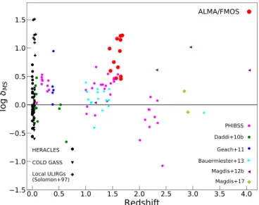
samples. In Figure 3, we also include our ALMA/FMOS

starburst sample at z∼1.6. It is evident that this study improves the statistics with respect to the number of starbursts at z>1 with CO detections; this is also exemplified in Figure2 of Tacconi et al. (2017).

We mention that the published samples used in this analysis were chosen to well represent the molecular gas properties of star-forming galaxies over a wide redshift range for comparison with our high-z starbursts. There are additional samples that are available (e.g., Bothwell et al.2013; Combes et al.2013) but

not included here since our aim was not to present a comprehensive assessment of the field. For this, we refer the reader to the recent work by Tacconi et al. (2017).

3. ALMA Observations and Data Analysis

Seven galaxies were observed in Cycle 3 (Project

2015.1.00861.S) with 38−39 12 m antennas on 2016 March 4, 11, and 13. Slightly different configurations for each science block yielded an angular resolution between 1 7 and 1 8, slightly higher than the request of 3″. We selected spectral windows to detect 12C16O (2−1; νrest=230.538 GHz)

red-shifted into Band 3. Four base bands(Δν=1.875 GHz each) were configured to detect CO emission for multiple targets (2–3) at different redshifts within a single science block and provide a measure of the continuum as an additional science product. Standard targets were used for calibration(e.g., flux, phase, bandpass), including J0854+2006, J0948+0022, Calli-sto, and J1058+0133.

Based on ALMA data from another program(PI. E. Daddi;

Project 2015.1.00260), one target (PACS-472; R.A.=

10:00:08.95, decl.=02:40:10.8) has a clear CO emission line

Figure 2.SEDs of our Cycle 3 sample from IR to radio wavelengths(photometric data are shown in blue), with the best-fit model shown by the black curve. The model of the dust emission is given for both a warm(red) and a cool (purple) component that contributes to the mid- to far-infrared emission. The unobscured stellar emission is shown by the cyan curve. An AGN contribution(yellow) is negligible for all cases.

detection in Band 6 (private communication) that places the object at a higher redshift than that based on our FMOS spectra. This misidentification explains a lack of a CO detection at the expected observed frequency; thus, we remove it from the sample. In Table 1, we list the targets and give their physical characteristics(e.g., redshift, stellar mass, SFR).

Analysis of the interferometric data set is carried out using the standard analysis pipeline available with CASA Version 4.6 (McMullin et al.2007). We first generate an image of the CO

emission using the task “immoments” with a channel (i.e., velocity) width encompassing the full line profile as given in Table 2. The emission is then modeled with an elliptical Gaussian using the CASA tool “imfit” that returns a source centroid, deconvolved source size, and integrated flux. As a precaution, we confirm these measurements by fitting the

emission in the uv-plane and through an independent effort using GILDAS available in the MAPPING package.

4. Results

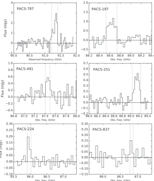
We detect CO at signal-to-noise ratio (S/N)>7 in five out of six galaxies observed in Cycle 3 (Figure 4; Table 2).

The line intensities(ICO) span a range of 0.26–1.64 Jy km s−1,

with the brightest source in CO emission attributed to our

most extreme outlier from the MS (PACS-787; SFR=

991 M_eyr−1). In Figure 5, the velocity profiles of the CO detections are shown in bins of either 100 or 200 km s−1. The majority have significant detections across multiple velocity bins. Overall, the strength of the CO emission is indicative of large amounts of molecular gas out of which deeply embedded stars are forming(see Section4.2).

All five sources with CO detections are essentially

unresolved with the beam sizes given in Table 2. However, we were able to measure a size for PACS-787 of 1 96±0 54 (16.6 kpc; FWHM−major axis)×1 02±0 39 (8.6 kpc; FWHM−minor axis) based on an elliptical Gaussian fit. We now know that the CO(5−4) emission from PACS-787, based on higher-resolution imaging with ALMA in Band 6, is nearly equally distributed between two galaxies undergoing a major merger, each with compact(r_1/2∼1 kpc) disks and having a separation of 8.6 kpc(Silverman et al.2018).

PACS-837 does not have significant emission in either CO or the continuum, although there is a tentative CO detection (0.42 ± 0.20 mJy) of 2.1σ significance at the expected spatial location and redshift (zCO=1.6569). For these reasons, we

include a panel for this object in Figures4and5. In subsequent analyses, we have derived a 3σ upper limit that places important constraints on our characterization of the CO properties of the sample since it should have been detected at a higher significance if it had CO properties similar to starburst galaxies given their LTIR.

Below, we present derived quantities such as CO luminosity, gas mass, and gas depletion time as a function of SFR and stellar mass. To aid in the interpretation of our results, we also

Table 1 Starburst Samplea

ID R.A. Decl. zspec

b

log Mstellar

c

LIRTotal SFR(IR) logδMS

d (Me) (Le) (Meyr−1) 787 10:02:27.95 02:10:04.4 1.5234 10.56 12.83±0.04 991-+8796 0.8 197 10:01:34.46 01:58:47.7 1.6005 10.75 12.58±0.06 551-+7283 0.7 491 10:00:05.16 02:42:04.7 1.6366 10.35 12.50±0.08 463-+8096 0.9 224 09:58:56.51 02:03:47.5 1.6826 10.05 12.51±0.10 467-+96121 1.2 251 10:02:39.63 02:08:47.2 1.5847 10.05 12.45±0.10 409-+81101 1.2 837 10:00:36.31 02:21:17.5 1.6552 9.98 11.72±0.12 76-+1925 0.5 299 09:59:41.31 02:14:42.8 1.6467 10.09 12.53±0.15 497-+147208 1.2 325 10:00:05.53 02:19:42.83 1.6557 10.39 12.05±0.22 162-+64106 0.4 819 09:59:55.54 02:15:11.46 1.4449 10.37 12.56±0.05 533-+6068 1.0 830 10:00:08.73 02:19:02.47 1.4610 10.68 12.45±0.06 412-+5462 0.6 867 09:59:38.10 02:28:57.06 1.5673 10.75 12.38±0.18 353-+119179 0.5 164 10:01:30.42 01:54:12.50 1.6489 9.94 12.33±0.28 309-+145274 1.1 Notes. a

The horizontal line differentiates between galaxies observed in Cycles 1(below) and 3 (above) with the exception of PACS-164, which was observed with NOEMA. b

Spectroscopic redshifts are based on Hα and have errors sDz (1+z)=1.8 ´ 10-4. c _{s ~ 0.07}

M dex error on the stellar mass(Ilbert et al.2015). d _d

MS=sSFR/ásSFRMSñ.

Figure 3.Compilation of samples from the literature used in this analysis with their redshifts and elevation above the MS as parameterized byδMS=sSFR/

ásSFRMSñand described in Section4. Our ALMA sample of 12 starbursts is shown by the larger red circles. Further details are provided in the text, including a more extensive set of references to these data sets.

present these measurements normalized to the expected value for MS galaxies at their respective redshift and stellar mass using average relations available from the literature. In particular, the expected value of the CO luminosity for MS galaxies (á ¢L_CO,MSñ) is based on Equation (1) of Sargent et al.

(2014), which depends on the LTIR of each galaxy. A similar

relation is given in Equation(4) of Sargent et al. (2014) for the

mean molecular gas mass of MS galaxies as a function of SFR. We then compare these normalized quantities as a function of their sSFR relative to the mean sSFR (ásSFRMSñ) of MS galaxies at an equivalent redshift and stellar mass such that δMS=sSFR/ásSFRMSñ. This normalization scheme applies to all figures that present the measurements in terms of δMS

including Figure 3. For our ALMA starbursts at z∼1.6, we use the MS relation as given in Equation (1). To show the

effect of using a different parameterization of the MS at z∼1.6, we also show results using the definition of the MS from Speagle et al.(2014) in the following subsection only. For

the comparison sample, we use the parameterization of

(M z)

sSFR stellar, as given in Equation (A1) of Sargent

et al.(2014).

4.1. CO-to-TIR Luminosity Relation

We revisit the relation between the CO luminosity LCO¢ and LTIRfor starbursts as reported by many studies (e.g., Magdis

et al.2012a; Sargent et al.2014). For our sample, the CO line

luminosity is calculated as follows and given in units of K km s−1pc2: n ¢ = ´ ´ D + ( ) ( ) L S v D z 3.25 10 1 , 2 L 7 CO 2 3 obs 2

where SCOΔv is the line flux in units of Jy km s−1, DL is the

luminosity distance in Mpc, and νobs is the observed line

frequency in GHz. We then convert the luminosity to the value of the J=1 -0 transition using LCO 2 1¢ ( - )/ ¢LCO 1 0( - ) =0.85 (Daddi et al. 2015). As mentioned above, LTIR is determined

from an integral of the best-fit model over 8–1000 μm, which tightly correlates with the obscured SFR (Kennicutt 1998).

Before introducing additional uncertainties with converting to physical units, we point out that these quantitiesL_CO¢ and LTIR

are essentially based on flux measurements and distance measures from their spectroscopic redshifts, with the exception

of converting between CO transitions. This allows us to establish observable trends independent of conversion factors to quantities such as gas mass and SFR, which will be presented in the following section.

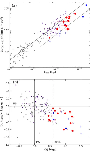
We plot LCO¢ versus LTIR for our starburst galaxies

(Figure6(a)) and a comparison sample of galaxies as described

in Section2.4. The well-established linear relation(solid line) is seen for which all MS galaxies lie along (Sargent et al.

2014). As presented by others (e.g., Solomon et al.1997; Daddi et al.2010b; Genzel et al.2010), the local ULIRGs (shown by

the blue plus signs) are offset from this relation with lower CO luminosities at a given LTIRas further illustrated by a parallel

relation (dashed line), a factor of 3×below the MS relation. Pertaining to our high-z starbursts, the entire ensemble(large red symbols) is visibly displaced to lower ¢LCO than expected for MS galaxies at their respective LTIR, even though a few

galaxies do fall close to(but below) the mean relation for MS galaxies. While some of our high-z starbursts lie along this parallel track (dashed line) to the MS, similar to the local ULIRGs, our sample appears tofill in the region between the MS and local starburst galaxies and thus is not as extreme in its difference from the MS galaxies.

In Figure 6(b), we illustrate that the decrement in CO

luminosity for high-z starbursts is larger with increasing boost in SFR above the MS by plotting this quantity as a function of sSFR, with each quantity normalized to the mean value of the star-forming MS population as described above. As shown in the figure, there is a general decline in ¢L_CO/á ¢L_CO,MSñ with increasing dMS. Since there are no clear signs of a gap in the ratioL_CO¢ /á ¢LCO,MSñbetween the MS and starburst galaxies, we argue that this decline is continuous in these parameters. This result appears to be valid even if using the parameterization of the MS at z∼1.6 from Speagle et al. (2014) that shows

slightly higher boost factors. These results are likely enabled by our selection of starbursts that includes those with milder offsets from the MS as compared to the local ULIRGs, thus effectively filling the gap seen in other studies (Daddi et al.2010b; Genzel et al.2010).

Based on a Kolmogorov–Smirnov test, there is only a probability of 0.07% of randomly drawing values of

¢

LCO/á ¢LCO,MSñ from the distribution of normal star-forming galaxies that matches the distribution of our starbursts with

á ñ >

sSFR sSFRMS 4. Furthermore, the difference in the mean

Table 2

ALMA Cycle 3 CO(2−1) Measurements

ID R.A. Decl. zCOa ICOb Δvc LCO¢

d _{Beam s}

rmsf

(CO) (CO) Sizee

787 10:02:27.954 +02:10:04.40 1.5249 1.64±0.20 600 10.69 2.67×1.79 (67.0) 0.085 197 10:01:34.461 +01:58:47.69 1.6016 1.086±0.088 700 10.55 2.11×1.79 (−69.6) 0.117 491 10:00:05.164 +02:42:04.69 1.6358 0.295±0.038 300 10.00 2.16×1.73 (−69.0) 0.067 224 09:58:56.515 +02:03:47.70 1.6826 0.262±0.034 400 9.98 2.39×2.02 (63.3) 0.026 251 10:02:39.626 +02:08:47.19 1.5863 0.413±0.040 700 10.12 2.36×2.01 (62.4) 0.040 837 10:00:36.233 +02:21:18.08 1.6572 0.127±0.061 300 <9.66 2.38×2.02 (62.8) 0.026 Notes. a σz=0.0003–0.0004. b Units of Jy km s−1. c

Full width of the CO line at zero intensity in units of velocity(km s−1). d

Log base 10; units of K km s−1pc2. e

Units of arcseconds(position angle in degrees). f

of theLCO¢ /á ¢LCO,MSñdistribution between typical galaxies and our starburst sample is significant at the 13σ level. This decline of theLCO¢ /LTIRratio suggests that starburst galaxies are able to

sustain high levels of star formation without the need for a larger gas supply, hence supporting a scenario of a higher SFE (=SFR/Mgas; see below) in a continuous manner from MS

galaxies to the most extreme starbursts as seen in the local ULIRGs. As an alternative explanation, if molecular clouds in starbursts are simply denser than MS galaxies, the reduced CO luminosity may be attributed to the lower surface area of the clouds since CO lines are optically thick.

4.2. Total Molecular Gas Mass

We expand on the above results by converting the CO luminosity, LCO 1 0¢ ( _- ), to the total molecular gas mass (Mgas)

using a scale factor (αCO) as routinely done in the literature

(Bolatto et al. 2013). A single value of this factor

(αCO=1.3 Me/(K km s−1pc2)) is applied across our starburst

sample. This estimate of αCO is based on a dynamical

assessment of the gas mass using a higher-resolution

observation with ALMA of CO(5−4) emission from

PACS-787(Silverman et al.2018). This value of αCOis similar to that

reported in the literature for local (Sargent et al. 2014) and

high-redshift starburst galaxies (e.g., Hodge et al. 2015),

including two other cases in our sample (Silverman et al.

2015a). We recognize that different values of αCOhave been

assumed in the literature. For example, Tacconi et al. (2017)

use a single value of αCO=4.36 (slightly depending on

metallicity) for all MS and starburst galaxies alike (i.e., for all δMS values). To assess the impact of this difference on our

results, we present our analysis in all subsequent plots also with this higher value for αCO=4.36 Me/(K km s−1pc2) and

discuss the implications in Section 5. We highlight that the uncertainty on the appropriate value of αCO is the dominant

systematic error in our measure of derived properties that include the molecular gas mass.

In Figure7(a), we plot the molecular gas mass as a function

of stellar mass for our high-z starbursts along with comparison samples (Section 2.4). Gas masses for the ALMA starbursts

(filled red circles) range between 1.4 and 7.5×1010_M e,

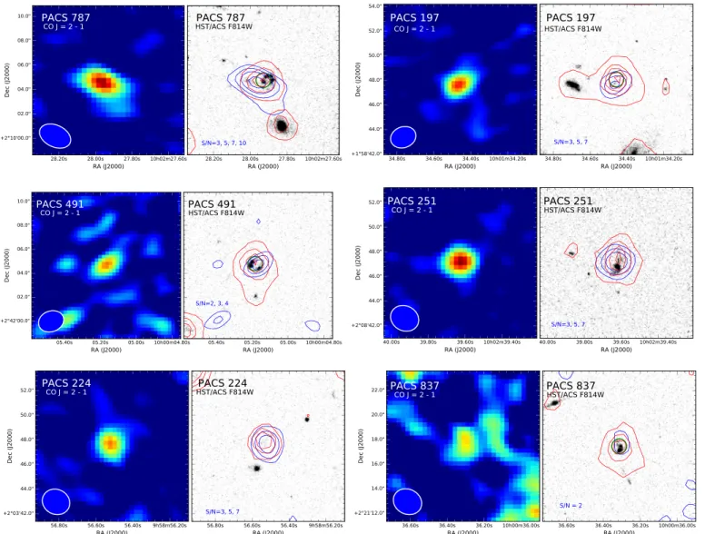
Figure 4.CO(2−1) maps of six high-z starbursts observed by ALMA in Cycle 3 (color panels on left). The shape of the ALMA beam is displayed in each panel. The minimumflux level is set at 0.5×σrms(Table2). Right panels: grayscale images of each starburst, from the COSMOS HST/ACS F814W mosaics (Koekemoer et al. 2007). CO emission is indicated with blue contours in steps of S/N as shown in each panel. Red contours indicate Spitzer/IRAC 3.6 μm detections that are typically

cospatial with the CO emission, indicating a close association between gas, obscured star formation, and the peak of the stellar mass distribution. The green circle in each HST panel marks the position of the FMOSfiber with a diameter of 1 2.

comparable to or even exceeding their mass in stars, as indicated by the slanted solid line. As expected, these gas masses are substantially higher than low-redshift SF MS galaxies (gray circles) and starbursts (blue plus signs). High-z SF MS galaxies(small triangles in purple) and the limited high-z starburst samples (blue squares), with αCO estimates, have

similar values of Mgas/Mstellarto our ALMA starbursts.

In Figure 7(b), we compare the ratio μ=Mgas/Mstellar,

relative to that of SF MS galaxies (μMS), to our reference

samples and the best-fit analytic expression given in Tacconi et al.(2017) as indicated by the green slanted line. The relative

gas fraction is plotted as a function of the boost in sSFR relative to SF MS galaxies, as done in Figure 6(b). By

comparing the ALMA starbursts (filled red circles) to the relation from Tacconi et al. (2017), high-z starbursts have

similar gas content to the more typical star-forming galaxies (Daddi et al.2010a; Tacconi et al.2010), counter to studies that

favor higher gas fractions (Genzel et al. 2015; Scoville et al.

2016; Lee et al.2017). We remark that this result is based on

the implementation ofαCO=1.3 Me/(K km s−1pc2). The use

of a higher value of 4.36 M_e/(K km s−1pc2) for our high-z starbursts, as discussed further below, results in close agreement with the Tacconi et al. (2017) relation.

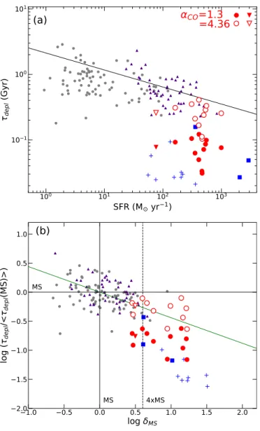
4.3. Gas Depletion Times/Star Formation Efficiency With estimates of the gas mass, we can measure the efficiency of forming stars (SFE=SFR/Mgas) and its inverse,

the time to deplete its gas reservoir if forming stars at a constant rate(τdepl=1/SFE) without gas replenishment. In Figure8(a),

we plot τdepl as a function of SFR, comparing our high-z

starbursts(filled red circles) to the reference samples described above. Wefind that our starburst sample has short gas depletion times ranging from ∼40 to 100 Myr (Table 3) that fall

significantly offset from MS galaxies (∼0.4–1 Gyr) at a given SFR.

In Figure8(b), the depletion times of our high-z starbursts

drop even further from that of SF MS galaxies with increasing distance above the SF MS as quantified as δMS.

The departure is still evident when comparing our data (red filled circles) to the analytical relation given in Tacconi et al.(2017) as indicated by the slanted green line. Based on

these results, we reinforce our hypothesis put forward in Silverman et al.(2015a) that the SFE (or gas depletion time)

increases (decreases) with distance above the MS stronger than any increase in the gas fraction, even if a mild increase is present.

Figure 5.CO(2−1) spectra for the Cycle 3 ALMA sample. Observed velocity channels are binned in intervals of 100 (PACS-787, 197, 491, 251) or 200 (PACS-224, 837) km s−1. Spectra were extracted with different apertures for each source chosen to closely represent the unresolved(i.e., peak) CO emission. The vertical dotted lines indicate the velocity interval over which the total CO luminosity is measured as given in Table2. The horizontal line marks the zero level.

5. Discussion

As with all CO studies of the molecular gas content, the essential inescapable issue is the conversion factor

αCO. As presented above, we have used a value of

1.3 M_e/(K km s−1pc2) based on a dynamical mass estimate from a higher-resolution CO image of PACS-787(Silverman et al.2018) that is broadly consistent with estimates from two

other cases in our high-z starburst sample (Silverman et al.

2015a). This value is not too dissimilar to that used for local

starbursts (i.e., αCO= 0.8 Me/(K km s−1pc2); Bolatto

et al. 2013) and even actively star-forming regions of z∼2

galaxies (e.g., Tadaki et al.2017).

As mentioned above, our assessment ofαCOrelies on a 0 3

resolution map of PACS-787, acquired through a Cycle 4 ALMA program, which has revealed two galaxies in the process of merging with CO detections for each galaxy at a high S/N. While in an early stage of a merger, both galaxies have maintained their molecular gas disks, thus enabling us to extract the gas mass from the dynamical mass with assumptions given in the aforementioned paper. It is possible that the value of the conversion factor used here induces a systematic level of uncertainty on the resulting gas masses. One issue may be that there is not definitive evidence for all starburst events within our sample as being triggered by a major merger, particularly at the same stage as PACS-787 in an evolutionary merger

Figure 6. (a) CO (1−0) luminosity ( ¢LCO) as a function of total infrared luminosity(LTIR) and (b) CO luminosity and sSFR both normalized to the

mean value of typical star-forming MS galaxies as described in the text. Red (filled) data points mark our 12 high-z starbursts. The inverted triangle represents the 3σ upper limit for PACS-837. The red open symbols are equivalent to the redfilled symbols with the exception that the value of δMSis

in reference to the star-forming MS of Speagle et al. (2014). From the

compilation of Sargent et al.(2014) as described in Section2.4, the small gray circles(purple triangles) represent star-forming MS galaxies at z<1 (z>1), while blue symbols show the local ULIRGs(plus signs) and high-z starbursts (filled blue squares). In panel (a), the best-fit relation to MS galaxies is shown by the solid line with a similar relation shifted 3×lower to indicate the location of local ULIRGs(Sargent et al.2014).

Figure 7.Molecular gas mass of high-z starbursts.(a) Log of the molecular gas mass as a function of the log of the stellar mass. Our ALMA starburst sample is shown by filled (open) red symbols, assuming the value of αCO to be 1.3

(4.36) Me/(K km s−1pc2), and an inverted triangle indicates an upper limit on the gas mass. Slanted lines indicate increasing values of Mgas/Mstellar as

marked. Additional starburst galaxies from the literature(listed in Section2.4)

withαCOmeasurements are included at low(blue plus signs) and high (blue

squares) redshift. Small gray circles represent low-redshift (z<0.3) MS star-forming galaxies, while high-z (z>1) MS galaxies are marked by purple triangles.(b) Molecular gas mass vs. sSFR, with both quantities normalized to the mean value of SF MS galaxies, at the equivalent stellar mass. The parameter on the abscissa,δMS, is the same as in Figure6(b). The slanted green

line is the average relation as reported in Tacconi et al.(2017). The gray circles

in the bottom panel represent all SF MS galaxies at z<1, a less restrictive sample than in the top panel.

sequence. However, the majority of starbursts in our ALMA sample do have multiple emitting components in the rest-frame ultraviolet(e.g., 819, 830, 491) and optical (e.g., PACS-867, 299, 325, 164) as detected by the Hubble Space Telescope (HST) Advanced Camera for Surveys (ACS) and Spitzer (see Figure 2 of Silverman et al.2015a); thus, we presume that most

of our starbursts are undergoing some sort of an interaction or merging event. Still, there is always the possibility that the conversion factor may be larger. Therefore, we explore the impact of a higher conversion factor on our results. Tacconi et al.(2017) are advocating the application of a more universal

value (αCO=4.36 Me/(K km s−1pc

2_{), plus a metallicity}

dependence) for the analysis of large samples.

First, we assess the impact on the gas fractions and

depletion times if the CO-to-H2 conversion factor is

4.36 M_e/(K km s−1pc2). This value is similar to star-forming regions in our own Milky Way and nearby local galaxies (Bolatto et al.2013). As a result, the gas fractions, expressed

here as Mgas/Mstellar, will be appreciably higher with most

above unity since they will be dominated in their mass budget by the molecular gas. This is seen in Figure 7(a), where gas

mass is plotted as a function of the stellar mass. In Figure7(b),

the ratio of the gas mass to stellar mass is plotted as a function ofδMSas defined above. The new gas masses (open red circles)

are found to be in closer agreement to the relation from Tacconi et al. (2017) that shows an increase in gas mass fraction, as

compared to SF MS galaxies, with their boost in sSFR above the MS. In this scenario, the boost in SFR for starbursts would be attributed to both an increase in the gas fraction and the SFE. This is seen in Figure8(b), where the depletion times

are significantly shorter than SF MS galaxies for αCO=

1.3 M_e/(K km s−1pc2), while a higher CO-to-H2 conversion

factor results in depletion times that are relatively higher but still slightly shorter than MS galaxies at all redshifts.

In general, any application of a scale factor to a set of measurements based on a well-selected statistical sample should be based on an independent assessment of the validity of this factor using a representative subset of the sample. To achieve such assurance in the applicable value ofαCOto high-z

starbursts(selected as outliers above the star-forming MS), we have obtained ALMA observations at a spatial resolution of ∼1″ or below for three starbursts (Silverman et al. 2015a,

2018) that provide broadly consistent results for a low value of

αCO. However, we note that the normalization of the dynamical

mass estimate and the method to assess the errors differ between PACS-819/830 and PACS-787. For both cases, there remains uncertainty in these estimates, and further effort with ALMA is needed at higher resolution to improve the quality of the size measurements, inclinations, and presence of any inflow/outflow components to the CO emission.

In light of these uncertainties, we are confident that the main results of this study are robust when considering the observed quantities irrespective of the value ofαCO. In Figure6(a), it is

clear that the high-z starbursts are offset from the relation betweenL_CO¢ and LTIRfor MS galaxies. There appears to be a

continuous decline in the amount of CO-emitting gas with distance above the MS(Figure6(b)), thus supporting models of

such behavior(Narayanan et al.2012).

6. Final Remarks

The question whether starburst outliers from the MS owe their higher sSFR to a higher gas fraction or to a higher SFE(or

Figure 8.(a) Gas depletion time (τdepl=Mgas/SFR) of high-redshift starbursts

as a function of their SFR. The slanted black line is the best-fit relation from Sargent et al.(2014). (b) Gas depletion time vs. sSFR with both normalized to

average values for SF MS galaxies. An analytic form of this relation is provided by Tacconi et al.(2017) and shown here in green. Symbols in both

panels are the same as in Figure6. Table 3 Derived Physical Properties

ID log Mgasa Mgas/Mstellar τdeplb

787 10.88 0.9 76 197 10.74 1.0 99 491 10.19 0.7 33 224 10.16 1.3 31 251 10.31 1.8 50 837 <9.77 <0.6 <77 299 10.55 2.9 71 325 10.17 0.6 92 819 10.66 1.9 86 830 10.70 1.0 121 867 10.34 0.4 63 164 10.51 3.7 105 Notes. a

Units of Meand based onαCO=1.3.

b _{t = M} SFR;

combination thereof) remains an unsettled issue in the current literature. For example, Sargent et al. (2014) and Silverman

et al. (2015a) argue for a substantially higher SFE, with even

sub-MS gas fractions, whereas Scoville et al. (2016) support

the opposite notion of starbursts being primarily driven by a higher gas fraction in outliers compared to MS galaxies. More recently, scaling relations have been proposed that tend to combine both effects. Thus, Scoville et al. (2017) derive

scaling relations from their ALMA dust continuum observation according to which d = µ ( ) M SFR SFE 3 gas MS 0.70 and m= M µd - _{( )} M M , 4 gas stellar MS 0.32 stellar 0.7

respectively, from Equations(7) and (6) of Scoville et al. (2017). Therefore, the elevation of the sSFR over the MS

(δMS), at fixed stellar mass, is attributed to a combination of

both a higher gas fraction and a higher SFE, scaling as∼μ3and ∼SFE1.4_{, respectively. Given that the gas fraction is higher in}

MS lower-mass galaxies (scaling as Mstellar-0.7), upon a major merger a galaxy would find itself with a higher gas fraction compared to an MS galaxy with a stellar mass equal to the combined stellar mass of the merger, which, according to Scoville et al., explains the higher gas fraction that they derive for MS outliers.

The equivalent scaling relations given by Tacconi et al. (2017) using primarily CO data are somewhat different:

d = µ ( ) M SFR SFE 5 gas MS 0.44 and m= M µd - _{( )} M M . 6 gas stellar MS 0.53 stellar0.35

Hence, for starbursting outliers, they find a slightly lower dependence of δMS on SFE, as compared to Scoville et al.

(2017), along with a slightly higher dependence on gas fraction,

compared to MS galaxies of the same stellar mass. The higher gas fraction(a factor of ∼3 for extreme starburst with δMS=10)

could not be completely accounted for by simple merging, as above, because of theflatter dependence of μ on the stellar mass along the MS, as from Equations(3) and (5). To account for this

higher (molecular) gas fraction, one may invoke some conver-sion of HI to H2, as the circumgalactic HI reservoir could be

destabilized upon merging. Note that Tacconi et al.(2017) adopt

a universal αCO=4.36 Me/(K km s−1pc2) (scaled down with

increasing metallicity), for both MS and MS outliers.

As shown in Figure7(b), adopting our best-fit value from the

dynamical argument αCO=1.3 Me/(K km s−1pc2) results in

gas fractions for starburst galaxies that are on average similar to MS galaxies; hence, the elevation of sSFR is fully attributed to a higher SFE, with SFE∼δMS, and in extreme starbursters the

SFE should be up to∼30 times higher than on the MS. Sargent et al.(2014) argue that a lower gas fraction in starbursts would

be a natural result of their much shorter gas depletion time º_SFE-1_{, if on average they are caught midway through their}

starburst, having already consumed a major fraction of their gas reservoir. This implies that starbursts at high redshifts would nearly double their stellar mass during the starburst, which at first sight may conflict with the constraint according to which on a global scale starbursts contribute just ∼15% of star formation (Rodighiero et al.2011). However, one may argue

that only a fraction, say,∼1/3, of massive galaxies experience a merger-driven starburst.

Adopting αCO=4.36 Me/(K km s−1pc2) as shown in

Figure 7(b), the starbursts fall along the continuous extension

from the MS, thus indicative of a single mode of star formation, whereas departures from such relations are more evident when adopting different values ofαCOfor MS and starburst galaxies.

These examples illustrate how much divergence there is from the resulting interpretations of why starburst galaxies have elevated sSFRs, with a major role being played by the infamousαCO.

We are grateful for the support from the regional ALMA ARCs. J.D.S. was supported by the ALMA Japan Research Grant of NAOJ Chile Observatory, NAOJ-ALMA-0127 and by

JSPS KAKENHI Grant Number “JP18H04346”. This work

was supported by the World Premier International Research Center Initiative (WPI Initiative), MEXT, Japan. C.M., A.R., and G.R. acknowledge support from an INAF PRIN-SKA 2017 grant. W.R. is supported by the Thailand Research Fund/Office of the Higher Education Commission grant No. MRG6080294 and Chulalongkorn University’s CUniverse. G.M. acknowl-edges support from the Carlsberg Foundation, the ERC Consolidator Grant funding scheme (project ConTExt, grant No. 648179), and a research grant (13160) from Villum Fonden. N.A. is supported by the Brain Pool Program, which is funded by the Ministry of Science and ICT through the National

Research Foundation of Korea (2018H1D3A2000902). This

paper makes use of the following ALMA data: ADS/JAO.

ALMA#2012.1.00952.S, ADS/JAO.ALMA#2015.1.00861.S,

and ADS/JAO.ALMA#2016.1.01426.S. ALMA is a

partner-ship of ESO(representing its member states), NSF (USA), and NINS(Japan), together with NRC (Canada), NSC and ASIAA (Taiwan), and KASI (Republic of Korea), in cooperation with the Republic of Chile. The Joint ALMA Observatory is

operated by ESO, AUI/NRAO, and NAOJ.

Appendix

Location of CO-emitting Regions

In Silverman et al.(2015a), we reported that the CO sources

were usually offset from regions of rest-frame UV emission, as seen by the HST/ACS observations of COSMOS (Koekemoer et al.2007; Scoville et al.2007). However, the centroid of the

CO emission was always cospatial with the stellar mass distribution as traced by the Spitzer/IRAC 3.6–8 μm bands. To investigate the significance of CO/UV offsets in more detail, we use recently reprocessed HST/ACS mosaics (A. Koekemoer 2018, private communication) where the astro-metry is directly tied to the International Celestial Reference Frame(ICRF), thereby eliminating uncertainties from possible offsets in older catalogs previously used to align HST images. The astrometric comparisons with our new ALMA observa-tions corroborate the significance of CO/UV offsets found in our past results, as shown in Figure4. For example, PACS 251,

787, and 491 have UV emission (shown by the grayscale

image) offset from the CO emission (blue contours) but more closely associated with the IR emission(red contours). In fact,

the other two(PACS 197 and 224) have essentially no emission in the UV while being strongly detected by Spitzer. These results are in agreement with our recent studies (Silverman et al. 2015a; Puglisi et al. 2017) and many others on the

extremely dusty nature of starbursts (e.g., Smail et al. 2004; Ivison et al. 2010; Chen et al. 2015) where any UV or

rest-frame optical emission lines are emitted from regions of relatively low extinction, possibly close to the surface of embedded star-forming regions since the bulk (∼90%) of the star formation is only observed at infrared wavelengths or longer. ORCID iDs J. D. Silverman https://orcid.org/0000-0002-0000-6977 W. Rujopakarn https://orcid.org/0000-0002-0303-499X E. Daddi https://orcid.org/0000-0002-3331-9590 A. Renzini https://orcid.org/0000-0002-7093-7355 G. Rodighiero https://orcid.org/0000-0002-9415-2296 A. Puglisi https://orcid.org/0000-0001-9369-1805 M. Sargent https://orcid.org/0000-0003-1033-9684 C. Mancini https://orcid.org/0000-0002-4297-0561 J. Kartaltepe https://orcid.org/0000-0001-9187-3605 D. Kashino https://orcid.org/0000-0001-9044-1747 A. Koekemoer https://orcid.org/0000-0002-6610-2048 M. Béthermin https://orcid.org/0000-0002-3915-2015 G. Magdis https://orcid.org/0000-0002-4872-2294 T. Nagao https://orcid.org/0000-0002-7402-5441 M. Onodera https://orcid.org/0000-0003-3228-7264 D. Sanders https://orcid.org/0000-0002-1233-9998 F. Valentino https://orcid.org/0000-0001-6477-4011 References

Bolatto, A. D., Wolfire, M., & Leroy, A. K. 2013,ARA&A,51, 207

Bolzonella, M., Miralles, J.-M., & Pello, R. 2000, A&A,363, 476

Bothwell, M. S., Smail, I., Chapman, S. C., et al. 2013,MNRAS,429, 3047

Bournaud, F., Elmegreen, B., Teyssier, R., et al. 2010,MNRAS,409, 1088

Bruzual, G., & Charlot, S. 2003,MNRAS,344, 1000

Carilli, C. L., & Walter, F. 2013,ARA&A,51, 105

Carleton, T., Cooper, M. C., Bolatto, A. D., et al. 2017,MNRAS,467, 4886

Casey, C., Narayanan, D., & Corray, A. 2014,PhR,541, 45

Casey, C. M., Chapman, S. C., Neri, R., et al. 2011,MNRAS,415, 2723

Casey, C. M., Cooray, A., Killi, M., et al. 2017,ApJ,840, 101

Chen, C.-C., Smail, I., Swinbank, A. M., et al. 2015,ApJ,799, 194

Combes, F., García-Burillo, S., Braine, J., et al. 2013,A&A,550, A41

Daddi, E., Bournaud, F., Walter, F., et al. 2010a,ApJ,713, 686

Daddi, E., Cimatti, A., Renzini, A., et al. 2004,ApJ,617, 746

Daddi, E., Dannerbauer, H., Liu, D., et al. 2015,A&A,577, 46

Daddi, E., Elbaz, D., Walter, F., et al. 2010b,ApJL,714, L118

Danielson, A. L. R., Swinbank, A. M., Smail, I., et al. 2017,ApJ,840, 78

Dekel, A., & Burkert, A. 2014,MNRAS,438, 1870

Di Matteo, T., Springel, V., & Hernquist, L. 2005,Natur,433, 7026

Downes, D., & Solomon, P. M. 1998,ApJ,507, 615

Draine, B. T., & Li, A. 2007,ApJ,657, 810

Elbaz, D., Leiton, R., Nagar, N., et al. 2018,A&A,616, 110

Fensch, J., Renaud, F., Bournaud, F., et al. 2017,MNRAS,465, 1934

Geach, J. E., Smail, I., Moran, S. M., et al. 2011,ApJL,730, L19

Genzel, R., Tacconi, L., Lutz, D., et al. 2015,ApJ,800, 20

Genzel, R., Tacconi, L. J., Gracia-Carpio, J., et al. 2010,MNRAS,407, 2091

Hodge, J. A., Riechers, D., Decarli, R., et al. 2015,ApJ,798, 18

Hopkins, P., Hernquist, L., Cox, T., et al. 2006,ApJS,163, 1

Ilbert, O., Arnouts, S., Le, F., et al. 2015,A&A,579, 2

Ivison, R. J., Papadopoulos, P. P., Smail, I., et al. 2011,MNRAS,412, 1913

Ivison, R. J., Smail, I., Dunlop, J. S., et al. 2005,MNRAS,364, 1025

Ivison, R. J., Smail, I., Papadopoulos, P. P., et al. 2010,MNRAS,404, 198

Kashino, D., Silverman, J. D., Rodighiero, G., et al. 2013,ApJL,777, L8

Kashino, D., Silverman, J. D., Sanders, D. B, et al. 2017,ApJ,835, 88

Kennicutt, R. C., Jr. 1998,ARA&A,36, 189

Kennicutt, R. C., Jr., & Evans, N. J. 2012,ARA&A,50, 531

Kimura, M., Maihara, T., Iwamuro, F., et al. 2010,PASJ,62, 1135

Koekemoer, A., Aussel, H., Calzetti, D., et al. 2007,ApJS,172, 196

Lackner, C., Silverman, J., Salvato, M., et al. 2014,ApJ,148, 137

Laigle, C., McCracken, H. J., Ilbert, O., et al. 2016,ApJS,224, 24

Lee, N., Sheth, K., Scott, K. S., et al. 2017,MNRAS,471, 2124

Leroy, A. K., Walter, F., Sandstrom, K., et al. 2013,AJ,146, 19

Lotz, J., Davis, M., Faber, S. M., et al. 2008,ApJ,672, 177

Lutz, D., Poglitsch, A., Altieri, B., et al. 2011,A&A,532, 90

Magdis, G. E., Daddi, E., Béthermin, M., et al. 2012a,ApJ,760, 6

Magdis, G. E., Daddi, E., Sargent, M., et al. 2012b,ApJL,758, L9

Magdis, G. E., Rigopoulou, D., Daddi, E., et al. 2017,A&A,603, A93

Magnelli, B., Lutz, D., Santini, P., et al. 2012,A&A,539, 155

McCracken, H., Milvang-Jensen, B., Dunlop, J., et al. 2012,A&A,544, 156

McMullin, J. P., Waters, B., Schiebel, D., Young, W., & Golap, K. 2007, in ASP Conf. Ser. 376, Astronomical Data Analysis Software and Systems XVI, ed. R. A. Shaw, F. Hill, & D. J. Bell(San Francisco, CA: ASP),127

Narayanan, D., Bothwell, M., & Romeel, D. 2012,MNRAS,426, 1178

Papadopoulos, P. P., van der Werf, P., Xilouris, E., Isaak, K. G., & Gao, Y. 2012,ApJ,751, 10

Puglisi, A., Daddi, E., Renzini, A., et al. 2017,ApJL,838, 18

Renzini, A., & Peng, Y. 2015,ApJ,801, 29

Riechers, D. A., Cooray, A., Omont, A., et al. 2011,ApJ,733, 12

Rodighiero, G., Daddi, E., Baronchelli, I., et al. 2011,ApJL,739, L40

Rujopakarn, W., Rieke, G., Eisenstein, D. J., & Juneau, S. 2011,ApJ,726, 93

Saintonge, A., Kauffmann, G., Kramer, C., et al. 2011,MNRAS,415, 32

Sanders, D. B., & Mirabel, I. F. 1996,ARA&A,34, 749

Sanders, D. B., Salvato, M., Aussel, H., et al. 2007,ApJS,172, 86

Sargent, M. T., Béthermin, M., Daddi, E., & Elbaz, D. 2012,ApJL,747, L31

Sargent, M. T., Daddi, E., Béthermin, M., et al. 2014,ApJ,793, 19

Schinnerer, E., Smolčić, V., Carilli, C. L., et al. 2007,ApJS,172, 46

Scoville, N., Abraham, R. G., Aussel, H., et al. 2007,ApJS,172, 38

Scoville, N., Lee, N., Vanden Bout, P., et al. 2017,ApJ,837, 150

Scoville, N., Sheth, K., Aussel, H., et al. 2016,ApJ,824, 63

Silverman, J. D., Daddi, E., Rodighiero, G., et al. 2015a,ApJL,812, L23

Silverman, J. D., Daddi, E., Rujopakarn, W., et al. 2018, ApJ, in press (arXiv:1810.01595)

Silverman, J. D., Kashino, D., Sanders, D. B., et al. 2015b,ApJS,220, 12

Smail, I., Capman, S. C., Balin, A. W., & Ivison, R. J. 2004,ApJ,616, 71

Smolčić, V., Novak, M., Delvecchio, I., et al. 2017,A&A,602, 1

Solomon, P. M., Downes, D., Radford, S. J. E., & Barrett, J. W. 1997,ApJ,

478, 144

Speagle, J. S., Steinardt, C. L., Capak, P. L., & Silverman, J. D. 2014,ApJS,

214, 15

Swinbank, A. M., Papadopoulos, P. P., Cox, P., et al. 2011,ApJ,742, 11

Tacconi, L., Genzel, R., Neri, R., et al. 2010,Natur,463, 781

Tacconi, L. J., Genzel, R., Saintinge, A., et al. 2017,ApJ,853, 179

Tacconi, L. J., Neri, R., Genzel, R., et al. 2013,ApJ,768, 74

Tadaki, K., Kodama, T., Nelson, E. J., et al. 2017,ApJ,841, 25

Tan, Q., Daddi, E., Magdis, G., et al. 2014,A&A,569, A98

Tanaka, M., Hasigner, G., Silverman, J. D., et al. 2017, arXiv:1706.00566

Volonteri, M., Capelo, P. R., Netzer, H., et al. 2015,MNRAS,449, 1470

Walter, F., Brinks, E., de Blok, W. J. G., et al. 2008,AJ,136, 2563