HAL Id: hal-00302583
https://hal.archives-ouvertes.fr/hal-00302583
Submitted on 24 Mar 2005
HAL is a multi-disciplinary open access
archive for the deposit and dissemination of
sci-entific research documents, whether they are
pub-lished or not. The documents may come from
teaching and research institutions in France or
abroad, or from public or private research centers.
L’archive ouverte pluridisciplinaire HAL, est
destinée au dépôt et à la diffusion de documents
scientifiques de niveau recherche, publiés ou non,
émanant des établissements d’enseignement et de
recherche français ou étrangers, des laboratoires
publics ou privés.
Effects of the synoptic scale variability on the
thermohaline circulation
J. J. Taboada, M. N. Lorenzo
To cite this version:
J. J. Taboada, M. N. Lorenzo. Effects of the synoptic scale variability on the thermohaline circulation.
Nonlinear Processes in Geophysics, European Geosciences Union (EGU), 2005, 12 (4), pp.435-439.
�hal-00302583�
SRef-ID: 1607-7946/npg/2005-12-435 European Geosciences Union
© 2005 Author(s). This work is licensed under a Creative Commons License.
Nonlinear Processes
in Geophysics
Effects of the synoptic scale variability on the thermohaline
circulation
J. J. Taboada1and M. N. Lorenzo2
1Group of Nonlinear Physics, Faculty of Physics, Univ. of Santiago de Compostela, 15782 Santiago de Compostela, Spain
2Faculty of Sciences, Campus de Ourense, Univ. of Vigo, 32004 Ourense, Spain
Received: 19 November 2004 – Revised: 8 March 2005 – Accepted: 9 March 2005 – Published: 24 March 2005
Abstract. In this paper the effect of the synoptic scale vari-ability is analyzed using a simple atmosphere-ocean coupled model. This high frequency variability has been taken into account in the model adding white gaussian noise in variables related to zonal and meridional temperature differences. Re-sults show that synoptic scale frequency variability on lon-gitudinal heating contrast between land and sea can produce a collapse of thermohaline circulation when a threshold of noise is overcome. This result is significant because if syn-optic scale variability in the next century increases due to the climatic change an increment of the probability of this col-lapse could be produced.
1 Introduction
In the last decades it has been established (Rahmstorf, 2000) that termohaline circulation (THC) plays a main role regulat-ing North Atlantic climate. Its formation depends on North Atlantic surface water being sufficiently cold and salty to destabilize water column and produce deep water formation. In this way THC formation is very sensitive to air-sea heat exchange and freshwater input in North Atlantic. On the other hand these two parameters are expected to vary due to climate change produced by greenhouse gases accumula-tion in the atmosphere. The fate of THC under those new conditions has been the subject of a scientific debate since a work of Broecker (1987). This work warned for the first time about the possibility of a sudden climate change due to a switch in North Atlantic circulation driven by a freshening of surface water that would prevent formation of North At-lantic deep water (NADW). In a posterior work of the same author, Broecker (1997), THC was nominated the Achilles heel of actual climate, highlighting the possibility that minor changes in parameters can cause a sudden change in climate conditions. This hypothesis has been also sustained by the Correspondence to: J. J. Taboada
growing evidence from paleoclimatic archives of past abrupt climate changes (Stocker and Schmittner, 1997).
Many modeling studies have been done in the last decades in order to study the behavior of THC under a changing climate (Stocker and Schmittner, 1997; Rahmstorf, 2000; Stouffer and Manabe, 2003). Results are somewhat differ-ent, ranging from the possibility of a total collapse, to a rein-forcement of THC, but a common picture appears. This pic-ture shows that ocean-atmosphere system has more than one stable mode of operation. A schematic stability diagram can be found in Rahmstorf (2000), showing the nonlinear char-acteristic of THC that implies different responses to pertur-bations. Freshwater input appears as a key control variable for the THC.
The main uncertainties that must be overcome in these studies are, on the one hand to know exactly the actual evaporation-precipitation budget in North Atlantic. We must remind that in nonlinear systems this is a critical question, because depending on how close of the threshold we are, the behavior of the whole system facing the same perturba-tion will be very different. On the other hand, it is also very important to know the actual intensity of THC (Tziperman, 2000). WOCE project has obtained a value of 15±2 Sv that can be used as real value (Ganachaud and Wunsch, 2000).
The increasing rate of freshwater input (Stocker et al., 2001) and the location of this input are also important and unknown variables. Moreover in 3-D models it has been demonstrated that THC behavior depends greatly on vertical mixing parametrization (Knutti et al., 2000).
It is also necessary to know the “hydrological sensibil-ity” (Rahmstorf and Ganopolski, 1999), namely, the rate of change of hydrological cycle in a heating atmosphere. The problem of climate change itself is not yet well established and some quite surprising feedbacks can appear. In this way, Delworth and Dixon (2000) have proposed that in an scenario of global heating, NAO (North Atlantic Oscillation) would be preferably in the positive phase, enhancing North Atlantic winds. These enhanced winds will cause a cooling of surface water that can cancel the effects of freshening. On the other
436 J. J. Taboada and M. N. Lorenzo: Variability on the THC 3 1 2 Qs Qs q q q Ta1 Ta2 KT KT 800 m 4000 m EQ 45ºN 70ºN 3 1 2 Qs Qs q q q Ta1 Ta2 KT KT 800 m 4000 m EQ 45ºN 70ºN
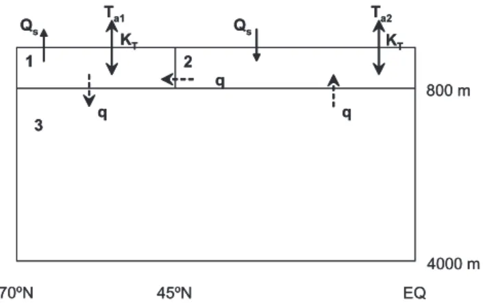
Fig. 1. Geometry of the North Atlantic through a 3-D box model. qrepresent the thermohaline circulation and the sense of the arrows indicates a positive circulation.
hand, Latif et al. (2000) have proposed a similar mechanism but with ENSO pattern.
In this way, we can see that 3-D fully comprehensive cli-mate models have some uncertainties, in particular in re-sponse to freshwater inputs (IPCC, 1999). Moreover, those models do not explicitly simulate synoptic variability, i.e. the main stochastic component of climate system. This unre-solved variability can be added as random fluctuations in pa-rameters or variables of the model. The role of these fluc-tuations could be decisive to regulate the transition between the different operation modes of the THC as occurs in other physical systems (Garc´ıa-Ojalvo and Sancho, 1999; Buceta et al., 2003; Ullner et al., 2003).
In this work we use a low complexity ocean-atmosphere coupled model to investigate the possibility of a collapse of thermohaline circulation taking into account the synoptic at-mospheric variability. These kind of models can only give qualitative results. But, the currently available computing capacity reduces the possibility of carry out exhaustive para-metric studies of the THC using 3-D models. In this way models of reduced complexity can make valuable contribu-tions to a better understanding of parameter space and they are also useful as an hypothesis builder.
The aim of the paper is to prove the ability of the model to provoke a collapse of the THC under some hypothesis such as a massive sudden freshwater input. Then we will look at the possibility of such a collapse adding noise in order to simulate synoptic variability.
2 Model
The atmosphere-ocean model used in this paper has been taken from a previously published work of Roebber (1995). The atmospheric part of the model is represented by a low-order model introduced by Edward Lorenz in 1984 and de-fined by three equations:
dX dt = −Y 2−Z2−aX + aF (1) dY dt =XY − bXZ − Y + G (2) dZ dt =bXY + XZ − Z , (3)
where X, Y and Z represent the meridional temperature gra-dient and the amplitudes of the cosine and sine phases of a chain of superposed large scale eddies, respectively. In Eq. (1), F represents the meridional gradient of diabatic heat-ing and in the Eq. (2) G is the asymmetric thermal forcheat-ing, representing the longitudinal heating contrast between land and sea, a=0.25 and b=4.
The ocean model considered is a three box model (Fig. 1) representing thermohaline circulation in the North Atlantic
ocean. In this model, Qs denotes the equivalent salt flux
(differential net surface evaporation), Ta1and Ta2 represent
restoring air temperatures with restoring constant KT, and q
is the magnitude of the thermohaline circulation. The sense of the circulation indicated denotes q positive. The explicit equations of the model and the ocean model constants are written in the work of Roebber (1995).
The atmospheric model is coupled to the ocean model through F and G that are allowed to vary in a seasonal cycle
F (t ) = F0+F1cosωt + F2(T2−T1) (4)
G(t ) = G0+G1cosωt + G2T1, (5)
where ω is the annual frequency and t =0 at winter sol-stice. The values chosen are, F0=4.65, F1=1, F2=47.9,
G0=−3.60, G1=1.0 and G2=4.0254. These assumptions
insure that F and G remain bounded by qualitatively plau-sible constraints for collapse flows (Roebber, 1995). On the other hand, the ocean is coupled to the atmosphere through the restoring temperatures Ta1and Ta2and the equivalent salt
flux (differential net surface evaporation) Qs with the next
expressions:
Ta1(t ) = Ta2−γ X(t ) (6)
Qs(t ) =0.00166 + 0.00022(Y2+Z2) , (7)
where γ =0.06364 and Ta2=25◦C are constants and the
parametrization of Qs(t )is due to the assumption that the
eddy water vapor transport is directly proportional to the eddy sensible heat flux given by Y2+Z2.
The Lorenz model that simulates atmosphere with the
cho-sen parameters has a chaotic behavior. The spectrum of
variability of this model is the typical one corresponding to a chaotic system. However, synoptic-scale spectrum is very different from chaotic spectrum (Gulev et al., 2002) and therefore the output of the Lorenz model can not be interpreted as synoptic scale variability in our case. To in-troduce the synoptic variability inside this model, i.e. the main stochastic component of climate system, we added ran-dom fluctuations in an additive way in parameters F and G. These fluctuations are given by white Gaussian noise with zero mean and whose correlation function is
1000 1500 2000 2500 3000 −10 −5 0 5 10 15 20 Time (years) Thermohaline Circulation (Sv) 1000 1500 2000 2500 3000 287.2 287.45 287.7 287.95 288.2 Time (years) T1 (K) 1000 1500 2000 2500 3000 291 291.25 291.5 291.75 292 Time (years) T2 (K) 1000 1500 2000 2500 3000 3.4 3.6 3.8 4 4.2 4.4 Time (years) T2 − T1 (K)
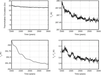
Fig. 2. Present-day steady state of the ocean-atmosphere system with active THC.
where A represents the noise intensity and 2A its variance. We have chosen this kind of noise parametrization because we are looking for the possibility that processes of a fre-quency higher than the considered in the model could pro-voke a collapse in thermohaline circulation. Moreover, the effect of atmospheric processes on the ocean has been taken into account in previous work as white noise (Frankignoul and Hasselmann, 1977).
3 Results
In a first study of the model we looked for the present-day state of the ocean-atmosphere system. This steady-state has an average temperature of 287.5 K in north hemisphere
lat-itudes ranging from 70◦N to 45◦N and 291 K in latitudes
from 45◦N to the equator. The strength of the THC is about
15 Sv (Fig. 2). This value was obtained changing the vertical exchange parameters in the ocean model in order to obtain a value near the measurements from hydrographical data gath-ered in the WOCE (World Ocean Circulation Experiment) (Ganachaud and Wunsch, 2000). The small variations ob-served in Fig. 2 are negligible versus a collapse of the THC. After the obtention of the present-day state, we searched for the possibility of a collapse of the THC under a mas-sive sudden freshwater input. In Fig. 3 we can see how THC collapses when we simulate a massive freshwater input. In this simulation, the equivalent salt flux of box 1, Qs1, was
forced to take a value greater than in the box 2, Qs2, in order
to simulate a Younger Dryas-like episode. In this figure we can see how THC collapses one hundred years after this pro-cess begins and when the model returns to present-day con-ditions, Qs1=Qs2=Qs(t ), THC does not recover in a next
future. This result means that the model is able to simulate a collapse of THC under feasible hypothesis like a Younger Dryas episode. 1000 1200 1400 1600 1800 2000 2200 2400 2600 2800 3000 −10 −5 0 5 10 15 20 Time (years) Thermohaline Circulation (Sv) 1000 1200 1400 1600 1800 2000 2200 2400 2600 2800 3000 275 280 285 290 295 Time (years) T1 (K)
Fig. 3. Effects of a massive freshwater input. Qs1=0.008 between
2000 and 2400 years, Qs2is given by equation (7).
10009 1500 2000 2500 3000 3500 4000 4500 5000 5500 6000 10 11 12 13 14 15 16 Time (years) Thermohaline Circulation (Sv) 0.0 0.04 0.1
Fig. 4. Effects of a stochastic perturbation on the meridional
gradi-ent of diabatic heating F for differgradi-ent values of the intensity of the applied noise A.
The main objective of this work is to consider if high-frequency variations in the meridional gradient of diabatic heating or in the longitudinal heating contrast between land and sea could induce significant changes in the ocean cir-culation. To carry out this study we run the model under present-day conditions (Fig. 2) with Qs1=Qs2=Qs(t ). To
simulate this variation we must remind that when modeling the low-frequency behavior of the climate system, the higher-frequency components can be parameterized as stochastic variables. In this way, we introduced stochastic perturba-tions of white gaussian noise in the parameters F and G of the model in an additive way and we analyzed their effects. In Fig. 4 we show the behavior of thermohaline circulation when the noise is added in F . In this case THC experi-ments a greater variability but it oscillates around 15 Sv and we don’t achieve a collapse of the THC. This result seems
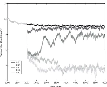
438 J. J. Taboada and M. N. Lorenzo: Variability on the THC 1000 1500 2000 2500 3000 3500 4000 4500 5000 5500 6000 −5 0 5 10 15 20 Time (years) Thermohaline Circulation (Sv) 0.0 0.04 0.4 0.43 0.5
Fig. 5. Effects of a stochastic perturbation on the zonal gradient in
diabatic heating G for different values of the intensity of the applied noise A.
understandable. F enters in Lorenz equation modifying
meridional temperature gradient X. In this way we can see in Eq. (6) that this “noisy” X introduces noise in the difference between temperature Ta1and Ta2. We must take into account
that this difference is by far greater than the noise introduced. Increments or decrements between northern and southern lat-itudes in North Hemisphere could strengthen or weaken the THC but a collapse would be very difficult because the basic differences between north and south are maintained. How-ever, if we introduce stochastic forcing in G we can detect a collapse of THC, when the stochastic component is suffi-ciently great. In Fig. 5 we can see that with the increment of the intensity of the forcing on G the THC is destabilized and after passing through an oscillatory transient state, with a fre-quency which corresponds to the diffusive time-scale of the ocean circulation years (Roebber, 1995), it collapses com-pletely. This collapse is related with the salinity in the ocean
because the parameter G is introduced in salt flux Qs and in
this case noise can be compared in magnitude with salt flux, meaning that it will be more significant. G represents the difference between the temperature in the land and the tem-perature in the ocean. An increment in the temtem-perature of the land can provoke a net freshwater flux into the northern part of the North Atlantic with the consequent loss of salin-ity and the collapse of THC. In the real climate that means that it is easier to collapse thermohaline circulation, chang-ing the budget evaporation-precipitation, than changchang-ing dif-ferences in temperatures. In other words, although the global warming by itself will not be able to collapse this circulation, the indirect effects (sudden freshwater inputs, more synoptic variability...) could help this collapse to be reached. It is important to remember that now noise is comparable to the signal. This means that if variability in the synoptic scale is comparable to variability in the climatic scale, THC could be eventually driven to a collapse.
1000 1500 2000 2500 3000 3500 4000 4500 5000 5500 6000 −4 −2 0 2 4 6 8 10 12 14 Time (years) Thermohaline circulation (Sv) 0.0 0.3
Fig. 6. Effects of a stochastic perturbation on the zonal gradient in
diabatic heating G after a weakening of the THC due to a increas-ing of the CO2concentration for two values of the intensity of the applied noise A.
Finally, owing to the fact that THC is very sensitive to parameters like atmospheric greenhouse gases concentration we have also analyzed the consequences of an increment of these gases. It has been established (IPCC, 1999) that tem-perature differences between polar and equatorial latitudes will decrease in a global warming context. In this way, we simulate the fate of THC under global warming, decreasing the value of γ that represents in the model those differences. In Fig. 6 we can see that these decreasing differences in tem-perature provoke a weakening in THC that eventually could achieve a total collapse if a threshold value is exceeded. But, even if this threshold is not exceeded in the next century, the weakening of THC implies that high-frequency synop-tic variations could provoke a collapse in THC easier than in actual conditions, as shown also in Fig. 6, where the neces-sary intensity noise to obtain a collapse of the THC is lower than in the Fig. 5.
4 Conclusions
Freshwater input seems to be a key parameter controlling THC behavior (Rahmstorf, 2000). The possibility of a mas-sive sudden freshwater input arising from disintegrating land ice sheets and mountain glaciers, must be taken into account because those massive inputs have been documented over some periods in the geological history (Clark et al., 2001). Those bursts of freshwater will stabilize the upper water col-umn and will affect deep water formation, reducing the abil-ity of its water to sink.
In this work, with a simple model, we can see that with an reasonable hypothesis, that increases freshwater input in North Atlantic in the same rate as did in Younger Dryas, THC undergoes a collapse that decrease average temperatures in
North Atlantic by 5◦C. This test has been done to prove the
ability of the model to simulate an eventual collapse of THC. The next step of the study was to consider synoptic vari-ability inherent in all climate studies. This varivari-ability was simulated adding white noise to parameters of the model that take into account meridional and zonal temperature varia-tion. It is important to note that lack of predictability near thresholds implies that abrupt climate changes will always have more uncertainty than gradual climate change and high-frequency variability represented by white noise can take a main role in this kind of systems as has been demonstrated in other works (Ganopolski and Rahmstorf, 2002). In our case noise added to the parameter that represents meridional temperature variation does not have relevant effects in THC circulation. But noise added in the parameter that represents zonal temperature variation can cause a collapse of THC cir-culation. Although in actual conditions high-frequency vari-ability is not able to collapse THC if this circulation is pro-gressively weakening by global warming, the intensity of noise necessary to provoke the collapse diminishes and this synoptic variability could help THC to collapse. On the other hand, climate change will have as a consequence an increase in extreme events, increasing in this way the synoptic vari-ability.
As a general conclusion we could state that we have used a simple model that gives only qualitative results, but can be taken into account as hypothesis builder. The hypothesis of this work is that the probable increase of synoptic variability in the next century can contribute to an eventual collapse of the THC.
Acknowledgements. Financial support from the Department of
Environment of the Galician Government (Xunta de Galicia) is gratefully acknowledged.
Edited by: A. Provenzale Reviewed by: two referees
References
Broecker, W. S.: Unpleasant surprises in the greenhouse, Nature, 328, 123–127, 1987.
Broecker, W. S.: Thermohaline Circulation, the Achilles’ Heel of Our Climate System: Will Man-Made CO2Upset the Current
Balance?, Science, 278, 1582–1588, 1997.
Buceta, J., Iba˜nes, M., Sancho, J. M., and Lindenberg, K.: Noise-driven mechanism for pattern formation, Phys. Rev. E, 67, 021 113 (1–8), 2003.
Clark, P., Marshall, S., Clarke, G., Hostetler, S., Licciardi, J., and Teller, J.: Freshwater Forcing of Abrupt Climate Change During the Last Glaciation, Science, 293, 283–287, 2001.
Delworth, T. L. and Dixon, K. W.: Implications of the recent trend in the Arctic/North Atlantic Oscillation for the North Atlantic thermohaline circulation, J. of Climate, 13, 3721–3727, 2000. Frankignoul, C. and Hasselmann K.: Stochastic Climate Models,
II. Application to SST Anomalies and Thermocline Variability, Tellus, 29, 289–305, 1977.
Ganachaud, A. and Wunsch, C.: Improved estimates of global ocean circulation, heat transport and mixing from hydrographic data, Nature, 408, 453–457, 2000.
Ganopolski, A. and Rahmstorf, S.: Abrupt Glacial Climate Changes due to Stochastic Resonance, Phys. Rev. Lett., 88, 038 501, 2002. Garc´ıa-Ojalvo, J. and Sancho, J. M.: Noise in spatially extended systems, Institute for Nonlinear Science, Springer-Verlag, New York, 1999.
Gulev, S. K., Jung. T., and Ruprecht, E.: Climatology and Interan-nual Variability in the Intensity of Synoptic-Scale Processes in the North Atlantic from the NCEP-NCAR Reanalysis Data, J. of Climate, 15, 8, 809–828, 2002.
IPCC: Climate change 2001: the scientific basis, in: Contribution of Working Group I to the Third Assessment Report of the Inter-governmental Panel on Climate Change, edited by: Houghton, J. T. et al., Cambridge University Press, Cambridge, UK, 881, 2001.
Knutti, R., Stocker, T. F., and Wright, D. G.: The effects of subgrid-scale parameterizations in a zonally averaged ocean model, J. Phys. Oceanogr., 30, 2738–2752, 2000.
Latif, M., Roeckner, E., Mikolajewicz, U., and Voss, R.: Tropical Stabilization of the Thermohaline Circulation in a Greenhouse Warming Simulation, J. of Climate, 13, 1809–1813, 2000. Rahmstorf, S.: The thermohaline ocean circulation – a system with
dangerous thresholds?, Clim. Change 46, 247–256, 2000. Rahmstorf, S. and Ganopolski, A.: Long-term global warming
sce-narios computed with an efficient coupled climate model, Clim. Change, 43, 353–367, 1999.
Roebber, P. J.: Climate variability in a low-order coupled atmosphere-ocean model, Tellus, 47A, 473–494, 1995.
Stocker, T. F., Knutti, R., and Plattner, G. K.: The oceans and rapid climate change: past, present, and future, Geophysical Mono-graph, 126, AGU, Washington D.C., USA, 2001.
Stocker T. F. and Schmittner, A.: Influence of CO2emission rates
on the stability of the thermohaline circulation, Nature, 388, 862–865, 1997.
Stouffer, R. J. and Manabe, S.: Equilibrium response of thermoha-line circulation to large changes in atmospheric CO2 concentra-tion, Clim. Dyn., 20 , 759–773, 2003.
Tziperman, E.: Proximity of the present-day thermohaline circula-tion to an instability threshold, J. Phys. Oceanogr., 30, 90–104, 2000.
Ullner, E., Zaikin, A., Garc´ıa-Ojalvo, J., and Kurths, J.: Noise-Induced Excitability in Oscillatory Media, Phys. Rev. Lett., 91, 180 601 (1–4), 2003.