HAL Id: insu-02088564
https://hal-insu.archives-ouvertes.fr/insu-02088564
Submitted on 3 Apr 2019
HAL is a multi-disciplinary open access
archive for the deposit and dissemination of
sci-entific research documents, whether they are
pub-lished or not. The documents may come from
teaching and research institutions in France or
L’archive ouverte pluridisciplinaire HAL, est
destinée au dépôt et à la diffusion de documents
scientifiques de niveau recherche, publiés ou non,
émanant des établissements d’enseignement et de
recherche français ou étrangers, des laboratoires
To cite this version:
Joris Heyman. TracTrac: A fast multi-object tracking algorithm for motion estimation. Computers
& Geosciences, Elsevier, 2019, 128, pp.11-18. �10.1016/j.cageo.2019.03.007�. �insu-02088564�
PII:
S0098-3004(18)31066-5
DOI:
https://doi.org/10.1016/j.cageo.2019.03.007
Reference:
CAGEO 4254
To appear in:
Computers and Geosciences
Received Date: 7 November 2018
Revised Date: 13 February 2019
Accepted Date: 22 March 2019
Please cite this article as: Heyman, J., TracTrac: A fast multi-object tracking algorithm for motion
estimation, Computers and Geosciences (2019), doi:
https://doi.org/10.1016/j.cageo.2019.03.007
.
This is a PDF file of an unedited manuscript that has been accepted for publication. As a service to
our customers we are providing this early version of the manuscript. The manuscript will undergo
copyediting, typesetting, and review of the resulting proof before it is published in its final form. Please
note that during the production process errors may be discovered which could affect the content, and all
legal disclaimers that apply to the journal pertain.
M
ANUS
CR
IP
T
AC
CE
PTE
D
TracTrac: a fast multi-object tracking algorithm
for motion estimation
Joris Heyman
Univ Rennes, CNRS
Géosciences Rennes, UMR 6118
35000 Rennes, France.
[email protected]
March 28, 2019
Abstract
1
TracTrac is an open-source Matlab/Python implementation of a robust and efficient
2
object tracking algorithm capable of simultaneously tracking several thousands of
3
objects in very short time. Originally developed as an alternative to particle image
4
velocimetry algorithms for estimating fluid flow velocities, its versatility and
robust-5
ness makes it relevant to many other dynamic sceneries encountered in geophysics
6
such as granular flows and drone videography. In this article, the structure of the
7
algorithmis detailed and its capacity to resolve strongly variable and intermittent
8
object motions is tested against three examples of geophysical interest.
M
ANUS
CR
IP
T
AC
CE
PTE
D
Keywords: Videography, Motion Estimation, Feature Tracking
10
1 Introduction
11
Owing to the popularization of digital cameras in the last 20 years, videography
tech-12
niques are increasingly used in the lab and in the field to measure velocities and
13
trajectories associated to a moving scenery. As earth processes are mostly dynamic,
14
imaging today appears as an affordable way to get spatio-temporal quantification of
15
these motions. Glacier motion, river flow, sediment transport, rock avalanches, wind
16
boundary layers, are some example of geophysical processes, whose understanding
17
rely deeply on how accurately their kinematics can be measured both in time and
18
in space. Yesterday restricted to laboratory studies with important experimental
19
apparatus (lasers, high speed cameras, computing clusters), flow imaging is now
20
expanding to in-situ monitoring of geophysical processes, notably thanks to the new
21
perspectives offered by drone videography [1]. In parallel, significant efforts have
22
been made in the computer vision community to improve and invent new image
23
processing algorithms treating efficiently these image sequences. Applications for
24
video surveillance (such as face recognition) and autonomous vehicles are among
25
the most spectacular achievements of these algorithms, running in real time [3, 14].
26
Curiously, few of these new methods were transferred into user-friendy, flexible and
27
open-source applications available for earth science researcher in their daily work
28
[5]. Processing images often costs much of the scientific effort instead of being a
29
powerful and direct mean to better understand natural processes. The present
arti-30
cle introduces TracTrac (see Computer Code Availability section), an open-source
31
Matlab/Python implementation of an original and efficient object tracking algorithm
32
capable of simultaneously tracking several thousands of objects in very short
com-33
putation time and very basic user knowledge. Its conception makes it equally good
34
for dealing with densely seeded fluid flows (typically treated with Particle Image
35
Velocimetry methods, PIV), granular flow, birds motion or any natural moving scene.
36
The article is structured as follows. After briefly reviewing the computational methods
37
that have been proposed for motion estimation in the past, TracTrac originality and
38
the algorithm structure is detailed. The accuracy and robustness of the algorithm is
39
then tested against a synthetic images occupied by artificial moving objects. Finally,
40
examples of TracTrac flow estimates are presented in real earth science applications
41
(turbulence, granular avalanche and bird flock).
42
2 Advances in motion estimation techniques
43
Literature about motion estimation from image sequence is vast and spreads over
44
several scientific disciplines, rendering difficult an exhaustive review. At least two
45
large families of methods have emerged: (i) the methods based on interrogation
46
windows, usually called Particle Image Velocimetry (PIV) and (ii) the methods based
47
on object detection and tracking, typically called Particle Tracking Velocimetry (PTV).
48
Although being not very informative, the choice of these acronyms refers to their
M
ANUS
CR
IP
T
AC
CE
PTE
D
initial use in films of flows seeded by tracer particles to establish a map of local
50
velocities. The spectrum of applications of PIV and PTV methods is however much
51
broader, extending to complex moving sceneries. The general idea behind PIV is
52
to quantify motion by cross-correlation of interrogation windows [25]. Dividing
53
the image into smaller boxes (typically of 8 or 16 pixels width), the local motion is
54
obtained by searching the box displacement that maximizes the cross-correlation
55
product of box pixel light or color intensities between two consecutive frames. In
56
contrast, PTV consists in detecting the presence of special features in an image and
57
tracking them through consecutive frames. Special features, also called objects,
58
can be particles (blobs of bright or dark intensities), but also more complex shapes
59
(corners, ball, faces, ...). Where PIV outputs a velocity vector for each interrogation
60
box, PTV provides the trajectory of an object (its position in successive frames)
61
which can be then mapped into a grid to get a dense velocity field [22]. In other
62
words, PTV takes the Lagrangian point of view of motion where PIV is essentially an
63
Eulerian vision. Both techniques have advantages and disadvantages as shown in
64
the following. While originally preferred for its relative simplicity and robustness (a
65
few free parameters involved), PIV inevitably introduces some filtering at fluctuation
66
scales smaller than the box size, which preclude the correct estimation of steep
67
velocity gradients. Partial recovering of interrogation boxes help at increasing velocity
68
map resolution but do not solve the filtering effect. Uncertainties are thus particularly
69
high for flows near walls and turbulent flows in general for which the Kolmogorov
70
scale can be small. In contrast, PTV is only limited by the scale of the tracked features
71
(particles, gradients) as well as their local density so that instantaneous velocity maps
72
are less prone to the box filter effect [10, 11]. Both PIV and PTV dynamic ranges
73
strongly rely on the accurate detection of peaks in the frames (e.g., the location
74
of the feature to track for PTV and maximum cross-correlation product for PIV).
75
Methods have been proposed to reach sub-pixel accuracy in peak location, allowing
76
for the measurement of displacements smaller than one pixel per frame. However,
77
local saturation of images (values equal to 0 or 1) and small particle image size may
78
produce peak locking and biased velocity measurements [6, 15, 16, 19, 20, 23]. To
79
minimize these effects, attention has to be taken to the effective dynamic range
80
reached (high contrasts) and the magnification factor of the lens. PIV methods
81
typically overtake PTV methods if particle displacement becomes large compared to
82
the mean inter particle image distance. A so-called particle spacing displacement
83
ratio p =pS/N /(v∆t) (with v∆t the particle image displacement, N the number
84
of particles and S the image surface) has been proposed by [13] to describe this
85
effect. To avoid ambiguities in the reconstruction of trajectories, PTV algorithms
86
generally requires high frame rates or low particle image densities, that is p ≥ 1. Thus,
87
PIV algorithms have often been preferred to probe densely seeded turbulent flows
88
where p can be small compared to 1. Combinations of the two methods have been
89
proposed to gain robustness in the case of large displacements (or large particle image
90
density) to limit the low-pass filtering effect of PIV [7, 21]. Another disadvantage of
91
PIV methods concerns complex sceneries made of moving and non-moving layers
92
(e.g. a flowing river on a fixed bed, a flock of flying birds through trees). The
cross-93
correlation procedure do not differentiate between layers so that the resulting velocity
94
is an average of the fixed and moving elements. In addition, incoherent motion
M
ANUS
CR
IP
T
AC
CE
PTE
D
such as Brownian motion or multiple wave celerities cannot be handled by most
96
PIV methods: at the scale of the interrogation window, the flow is supposed to be
97
continuous and unidirectional. In contrast, sharp interfaces between moving and
98
static regions, as well as non-coherent motions can in principle be rendered by PTV
99
methods [5]. There is today a net enthusiasm for PTV algorithms due to their broader
100
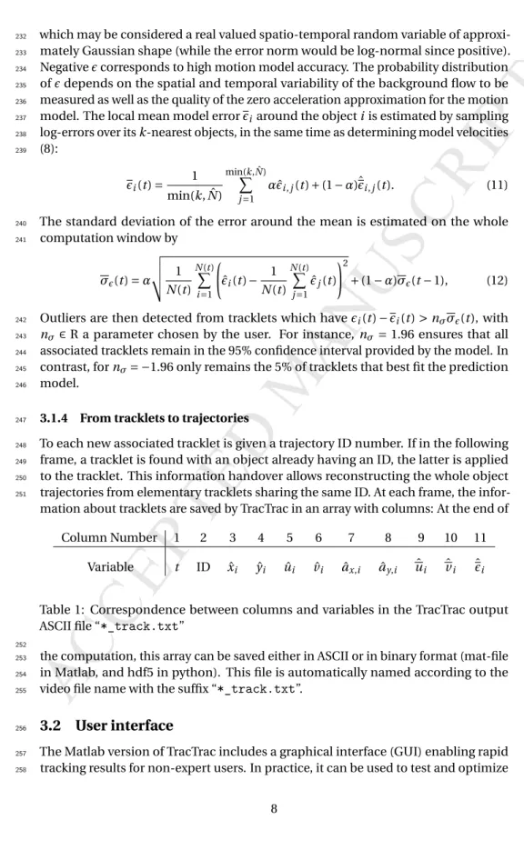
application range and their higher resolution [5, 9]. They are also directly transferable
101
to stereoscopic camera setup where the position and trajectory of objects can be
102
estimated in the three space dimensions [12, 13, 18]. However, most existing PTV
103
algorithms still suffer from the aforementioned drawbacks: (i) they are limited to large
104
particle spacing displacement ratio (p > 2 in [13] and in [5], while p>0.33 in a recent
105
study by [7]) and (ii) they are not computationally efficient when many features have
106
to be tracked (a maximum of 4000 particles per time frame are considered in [7] and
107
1000 in [5]).
108
3 TracTrac
109
The first innovation brought by TracTrac compared to traditional PTV methods is
110
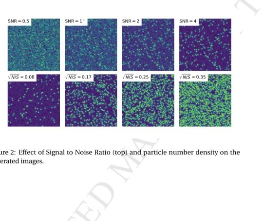
its efficiency. Indeed, TracTrac uses k-dimensional trees to search and compute
111
statistics around neighbouring objects [4], allowing very high analysis frame rate
112
even at large particle image number. The second key feature lie in an original
asso-113
ciation process of objects between frames, that significantly decreases the number
114
of erroneous trajectory reconstructions. This process is based upon a sequence of 3
115
frames (instead of 2 for classical pair association) and a conservative rule rejecting
116
any association ambiguities [21]. The third advantage of TracTrac is its capacity to
117
deal with high feature densities at relatively low acquisition frequencies (p down
118
to 0.25). This is achieved owing to a motion predictor step based on a local
spatio-119
temporal average of the neighbouring object velocities. Differences between the
120
motion prediction model and the observed displacement are systematically
moni-121
tored, allowing filtering outliers based on local and adaptive statistics of the motion
122
variability. This adaptive filter enables both the quantification of strongly incoherent
123
motions (of the Brownian motion type [5]) and coherent displacement (governed by
124
a spatio-temporal continuous deterministic velocity field) in the same image.
125
3.1 Details of the algorithm
126TracTrac rests on three main modules: object detection, motion estimation, error
127
monitoring.
128
3.1.1 Object detection
129
The first module regroups all the computing steps from the raw frame It to the 130
detection of the position of moving objects xt. Most of these preprocessing steps 131
are optional, and may be turned off by the user. The procedure is the following.
132
First a median box filter can be applied to remove possible noise on It. The default 133
size of this filter was set to 3 × 3 pixels. Second, the image is divided between a
M
ANUS
CR
IP
T
AC
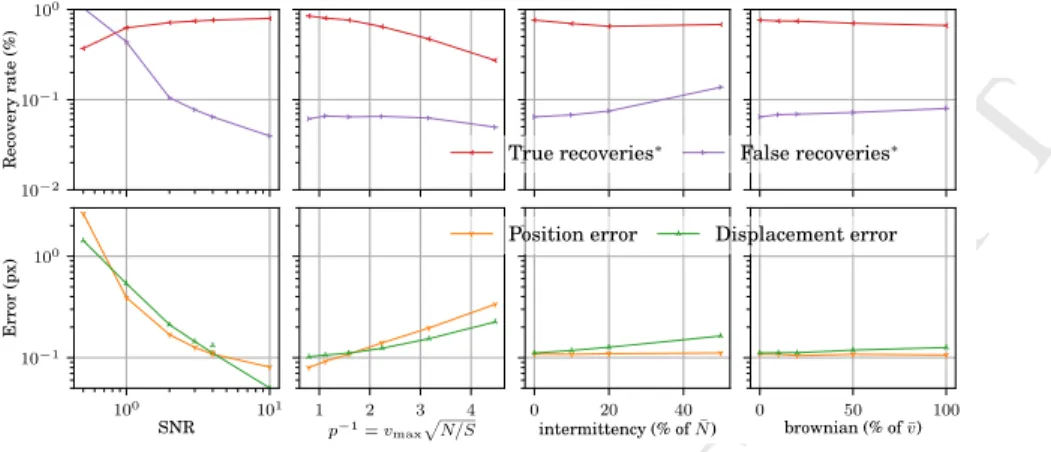
CE
PTE
D
“background” image Btmade of quasi-static regions, and a “foreground image” Ft, 135
formed by the moving regions. The latter is computed as Ft= It− Bt. This operation 136
allows focusing on the moving part of a scene, while ignoring the static regions. Bt 137
has to be recomputed at each frame. The method chosen here borrows from the
138
so-called “median” background subtraction method, where the background image is
139
taken to be a temporal moving average of pixel values:
140
Bt= β sign(It− Bt −1) + Bt −1, (1)
whereβ < 1 is the background adaptation speed. A large value of β gives backgrounds
141
that are rapidly adapted to the changes in scene luminosity. On opposite, a small value
142
ofβ provides background images that are insensible to rapid luminosity changes.
143
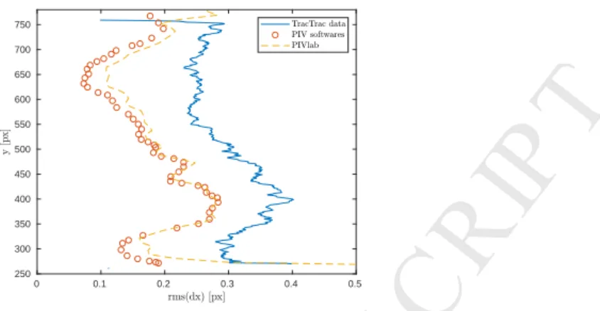
The default value is set toβ = 0.001. The recurrence relation (1) requires to provide
144
an initial guess for B0, which is computed from an average of the first 1/(2β) frames
145 B0= 2 β β/2−1 X t =0 It. (2)
It is worth noting that PTV methods are able to resolve sharp velocity gradients as
146
well as out-of-plane velocity gradients so that background subtraction may not be
147
always necessary. Objects are then identified in the foreground image by a so-called
148
“blob detection” method. TracTrac integrates two state-of-the-art detectors, namely
149
Difference of Gaussians (DoG) and Laplace of Gaussian (LoG), both depending on
150
a single scale parameterδ. The DoG convolves the image with a filter constructed
151
from the subtraction of two Gaussian of bandwidth 0.8δ and 1.2δ. It acts as a
band-152
pass filter selecting blobs in the 20% scale range aroundδp2. The LoG approach
153
first convolves the image with a Gaussian filter of bandwidthδ, then applying the
154
Laplacian operator on the convoluted image. Both approaches yield a filtered image
155
Ft0with a strong positive response in the presence of objects of scaleδ. Positions
156
of the object centroids {xt} are obtained by searching for local maximum in Ft0. To 157
minimize false detections, an intensity thresholdε is fixed under which maxima are
158
ignored. In TracTrac, the default value ofε is fixed to half standard deviation above
159
the mean luminosity of F0
t. Sub-pixel resolution of object position is achieved by 160
fitting a quadratic or a Gaussian function to the pixel intensity values around the
161
centroid position, and finding then the position of the maximum of this function. For
162
instance, if a maximum is found in pixel i , j , the sub-pixel position of object will be
163 x = j + F0 i , j +1− Fi , j −10 2(F0 i , j +1− 2Fi , j0 + Fi , j −10 ) , (3) y = i + F0 i +1,j− Fi −1,j0 2(F0 i +1,j− 2Fi , j0 + Fi −1,j0 ) , (4) (5) for a quadratic function. The formula is the same for a Gaussian function, replacing F0
164
by ln(F0). The ensemble of points xi(t ), i = 1,..., N (t) made of the sub-pixel centroid 165
positions are then tracked through time.
M
ANUS
CR
IP
T
AC
CE
PTE
D
3.1.2 Motion estimation 167As classical PTV algorithms [7, 13], motion estimation is achieved by associating
168
detected objects between successive frames, typically by minimization of Euclidean
169
distance. In TracTrac, at each time t , the set of N (t ) detected objects is organized
170
into a 2-dimensional tree allowing for fast nearest neighbour search [4]. The nearest
171
neighbours in successive frames are computed for both forward and backward time
172
association:
173
• forward xi(t ) → xj(t + 1): for each xi(t ), find its closest neighbour in {x(t + 1)}, 174
• backward xi(t + 1) → xj(t ): for each xi(t + 1), find its closest neighbour in 175
{x(t )}.
176
Since objects usually appear and disappear through frame, both computations may
177
give different results. In order to minimize false associations, only the unequivocal
178
pairs are kept (i.e., the pairs that point to the same objects regardless of the time
179
direction of association). In doing so, ambiguous associations are automatically
180
disregarded. A fragment of trajectory (“tracklet”) is defined if two consecutive and
un-181
equivocal associations are made for the same object. In other words, when a position
182
triplet xi(t − 1) ↔ xj(t ) ↔ xk(t + 1) is found without ambiguity, it is considered as a 183
valid fragment of trajectory, to which is associated a new or existing ID (depending
184
on whether the object has been already associated to a trajectory ID in the frame
185
t − 1). This 3-frame association technique reduces significantly the occurrence of
186
bad associations. In addition, it enables the computation of second order object
187
velocities (via central differences) as well as their accelerations:
188 ˆ v (t − 1) = x(t ) − ˆx(t − 2)ˆ 2∆t , (6) ˆ a(t − 1) = x(t ) − ˆx(t − 2) + 2 ˆx(t − 1)ˆ ∆t2 (7)
This technique does not increase the computational cost significantly since nearest
189
neighbour associations (xj(t ) ↔ xk(t + 1)) are saved for the following time step. In 190
the following, the variables pertaining to objects that were associated into tracklets
191
in the frame t are denoted by a hat (i.e., ˆx(t ), ˆN (t )). The quality of this association
192
step is often constrained by the maximum object displacement between consecutive
193
frames, or equally the maximum object velocity divided by the frame rate of the
194
camera. Indeed, erroneous associations spontaneously arise from aliasing effects
195
when object displacement is comparable to the average distance separating objects
196
(for instance, points on a line distant by 10 pixels that travel at 10 pixels per frame
197
will appear having a null velocity). Motion recognition is relatively easy when p−1=
198
v∆tpN /S ¿ 1 (or equally when p À 1 [13]). In TracTrac, this condition is relaxed by
199
the use of a predictor step based on a motion model inherited from previous time
200
step [7, 17]. In other words, TracTrac first predicts the position objects in the following
201
frame and then use this prediction to perform the following association. At time
202
t , the motion model is based on the pool of objects associated to tracklets at t − 1,
203
their velocities ˆv (t − 1) and their motion predictors ˆv(t − 1) (where the bar symbol
M
ANUS
CR
IP
T
AC
CE
PTE
D
Figure 1: Prediction-Association process between frames t , t + 1 and t + 2
stands for quantities related to the motion model). This information is passed to all
205
objects detected in the current frame t by a weighted average over their k-th nearest
206
neighbours taken from the aforementioned pool:
207 vi(t ) = 1 min(k, ˆN ) min(k, ˆN ) X j =1 αˆvi , j(t − 1) + (1 − α) ˆvi , j(t − 1). (8)
The weightα ∈ [0,1] introduces a finite temporal relaxation of the predicted velocities.
208
Forα → 1, the motion model is only based on the immediate previous frame, while
209
forα → 0, history of the velocities predicted in earlier frames are used to compute the
210
motion model. Averaging over the k-th nearest neighbours has two advantages. First,
211
it allows filtering the smallest spatial variations of velocities, that can be influenced
212
by noise or erroneous tracklets associations. Second, it naturally adapts to the local
213
density of objects, in contrast to fixed-size kernel smoothing methods: the larger the
214
density, the smaller the filtering scale, and the finer the prediction. Once the motion
215
model is computed, new object position is predicted assuming zero acceleration:
216
xi(t ) = xi(t − 1) + vi(t )∆t, (9)
and the association process is performed by searching among the nearest neighbours
217
between x(t ) and x(t + 1) (Fig. 1). These new tracklets can either be saved and the
218
following frame proceed, or used iteratively to refine the motion model and predict
219
once again object displacement. The predictor step is thus implemented as an
220
iterative sequence, using the temporary recovered tracklets as additional velocity
221
vectors considered in the motion model. Convergence is generally obtained after
222
a few iterations, the number of associated tracklet reaching a maximum. Once the
223
desired number of iteration is reached, computation continues with the following
224
frame.
225
3.1.3 Error monitoring and outliers filtering
226
The motion model used in TracTrac enables a continuous monitoring of the
differ-227
ence between predicted and actual displacements. This information is of particular
228
value since it helps to eliminate outliers from the obtained associations based on
229
statistical criterion. For each unequivocal associations, the log-error norm between
230
the predicted and the true velocity vector is
231 ²i(t ) = log ³° ° ° ˆ vi(t − 1) − ˆvi(t ) ° ° ° ´ . (10)
M
ANUS
CR
IP
T
AC
CE
PTE
D
which may be considered a real valued spatio-temporal random variable of
approxi-232
mately Gaussian shape (while the error norm would be log-normal since positive).
233
Negative² corresponds to high motion model accuracy. The probability distribution
234
of² depends on the spatial and temporal variability of the background flow to be
235
measured as well as the quality of the zero acceleration approximation for the motion
236
model. The local mean model error²i around the object i is estimated by sampling 237
log-errors over its k-nearest objects, in the same time as determining model velocities
238 (8): 239 ²i(t ) = 1 min(k, ˆN ) min(k, ˆN ) X j =1 αˆ²i , j(t ) + (1 − α)ˆ²i , j(t ). (11)
The standard deviation of the error around the mean is estimated on the whole
240 computation window by 241 σ²(t ) = α v u u t 1 N (t ) N (t ) X i =1 Ã ˆ ²i(t ) − 1 N (t ) N (t ) X j =1 ˆ ²j(t ) !2 + (1 − α)σ²(t − 1), (12)
Outliers are then detected from tracklets which have²i(t ) − ²i(t ) > nσσ²(t ), with 242
nσ∈ R a parameter chosen by the user. For instance, nσ= 1.96 ensures that all
243
associated tracklets remain in the 95% confidence interval provided by the model. In
244
contrast, for nσ= −1.96 only remains the 5% of tracklets that best fit the prediction
245
model.
246
3.1.4 From tracklets to trajectories
247
To each new associated tracklet is given a trajectory ID number. If in the following
248
frame, a tracklet is found with an object already having an ID, the latter is applied
249
to the tracklet. This information handover allows reconstructing the whole object
250
trajectories from elementary tracklets sharing the same ID. At each frame, the
infor-251
mation about tracklets are saved by TracTrac in an array with columns: At the end of Column Number 1 2 3 4 5 6 7 8 9 10 11
Variable t ID xˆi yˆi uˆi vˆi aˆx,i aˆy,i uˆi vˆi ˆ²i
Table 1: Correspondence between columns and variables in the TracTrac output ASCII file “*_track.txt”
252
the computation, this array can be saved either in ASCII or in binary format (mat-file
253
in Matlab, and hdf5 in python). This file is automatically named according to the
254
video file name with the suffix “*_track.txt”.
255
3.2 User interface
256The Matlab version of TracTrac includes a graphical interface (GUI) enabling rapid
257
tracking results for non-expert users. In practice, it can be used to test and optimize
M
ANUS
CR
IP
T
AC
CE
PTE
D
the free parameters meanwhile observing in real time their effect on the quality of
259
the tracking process. In contrast to the Matlab GUI, the Python version of TracTrac
260
can be launched either as a Python script or as a Python function. This command
261
line control allows treating iteratively several videos or integrating TracTrac directly
262
into Python scripts (a list of video files can also be chosen in the Matlab GUI). Full
263
compatibility is maintained between the two implementations owing to a common
264
input parameter file whose structure is given as the supplementary material. Details
265
about the Matlab GUI and the Python commands are also provided in this document.
266
4 Results and discussion
267
4.1 Synthetic flow
268In order to test TracTrac performances, synthetic images were created, enabling a
269
comparison of the algorithm predictions with known object trajectories. The flow
270
was chosen in order to test the algorithm robustness for both strongly unsteady and
271
non-uniform continuous flow field.
272
4.1.1 Flow description
273
The synthetic trajectories are initiated by N points randomly distributed in the image
274
(x0, y0). At each frame, a synthetic image is build by applying a Gaussian kernel
275
of fixed standard deviation on each object centroid. Uncorrelated noise is then
276
added to the image pixels with an intensity depending on the signal-to-noise ratio
277
(SNR) chosen (Fig. 2). An image is created at each frame, while advecting the objects
278
according to the following two consecutive operations: a first one operating in radial
279
coordinates (r =px2+ y2,θ = tan−1(y/x)):
280
rn+1 = rn, (13)
θn+1 = θn+ 4δ cos(nπ/50) exp(−0.5(rn/80)2) − 10δcos(nπ/25)exp(−0.5(rn/50)(14)2),
followed by a second step in cartesian coordinates (x = r cosθ, y = r sinθ):
281
xn+1 = xn+ 2δ sin(πn/100) ∗ yn+ ξn, (15)
yn+1 = yn+ δxn+ ξn, (16)
whereξnis a white noise term whose intensity will be varied. In practice, the time 282
stepδ = 0.01 is chosen to get displacement lengths in the range 0-20 pixels per frames.
283
Cartesian and polar coordinate systems are centred on the image centre. Periodic
284
boundary conditions are applied when a point leaves the image field. Snapshot of the
285
flow velocity vectors were plotted on Fig. 3. Before the next frame, a finite number of
286
points (0-50%) are associated new coordinates in order to mimic in and out of plane
287
motion.
M
ANUS
CR
IP
T
AC
CE
PTE
D
SNR = 0.5 SNR = 1 SNR = 2 SNR = 4 N/S = 0.08 N/S = 0.17 N/S = 0.25 N/S = 0.35Figure 2: Effect of Signal to Noise Ratio (top) and particle number density on the generated images.
t = 0
t = 30
t = 60
t = 90
Figure 3: Space dependence of the synthetic vortex flow considered (Eq. 8) at various time instants.
M
ANUS
CR
IP
T
AC
CE
PTE
D
10−2 10−1 100 Recovery rate (%)True recoveries∗ False recoveries∗
100 101 SNR 10−1 100 Error (px) 1 2 3 4 p−1= v max p N/S 0 20 40 intermittency (% of ¯N) 0 brownian (% of ¯v)50 100
Position error Displacement error
Figure 4: Algorithm accuracy function of 4 variables: Signal to Noise Ratio (SNR), object separation compared to mean displacement (p−1= vpN /S, with v the mean
displacement and N the number of objects in the area S), object appearance and disappearance (“Intermittency”) and velocities random fluctuations (“Brownian”). True recoveries rates are defined according to a maximum position error of d and a maximum displacement error of v/2. False recoveries are found for the opposite criterion. Default parameters are: SNR=4, N=1000, Intermittency=0 and Brownian=0.
4.1.2 Accuracy
289
Accuracy was measured owing to 4 indexes: mean percentage of true and false
290
object detection as well as mean absolute error in object position and displacement
291
estimation. These indexes were computed for various image qualities and flow
292
properties. To better isolate TracTrac performances, no pre-processing step was
293
performed on the synthetic images (e.g. background subtraction, median filter). First,
294
TracTrac accuracy is compared to the Signal to Noise Ratio (SNR, defined as blob
295
peak magnitude over magnitude of an underlying uniform noise). Results presented
296
in Fig. 4 show that increasing SNR significantly increases tracking quality: for SNR≥ 4
297
(a typical value in PIV experiments), less than 5% of false detections are made, while
298
mean position and displacement error are below 0.2 pixels, a value comparable with
299
recent PTV methods [7]. Another quality factor is given by the ratio of maximum
300
displacement length to the mean distance between neighbour objects expressed as
301
p−1= vmax/
p
N /S (the inverse of the ratio defined by [13]). PTV algorithm are usually
302
limited to r ¿ 1 to avoid object association ambiguities between frames [13, 17].
303
Thanks to the motion predictor, the association rule, and the outlier filter, false
304
detections remain below 6% for ratios p−1≈ 4.5, while position and displacement
305
error are below 0.5 pixels. To the author knowledge, such large values of p−1have not
306
yet been reported in the literature.
307
Appearance and disappearance of objects through time, referred to as
“intermit-308
tency” in Fig. 4, often occur due to out of transverse velocities in 3D flows observed on
309
2D planes. While this phenomenon complicates the association process, the number
310
of false tracklets remains limited to 12% at high intermittency levels (50% of the object
M
ANUS
CR
IP
T
AC
CE
PTE
D
0
10000
20000
30000
Number of object tracked N
0.0
0.2
0.4
0.6
Computation time per step [s]
Synthetic flow
PIV challenge
Granular Avalanche
Figure 5: Computation time per video frame depending on the number of objects tracked. Computations are made with the Python implementation of TracTrac on a HP ELiteBook 840 laptop with processor Intel i7.
disappearing at each frame), suggesting a good adaptation of the algorithm to out of
312
plane motions. While intermittency does not affect position error, it increases slightly
313
the mean displacement error (owing to false associations, with mean displacement
314
errors smaller than 0.5 pixel for a level of intermittency of 50%).
315
The last factor considered is the stochasticity of the underlying flow field, which
316
cannot be predicted by deterministic motion predictors [5]. To investigate this effect,
317
white noise was summed to object velocities in proportion of the deterministic flow
318
velocity magnitude. Fig. 4 shows that both false detection and displacement error
319
remain limited for fluctuations levels comparable with the average magnitudes (9%
320
and 0.3 pixel respectively). This good performance is ensured by the continuous and
321
local monitoring of prediction errors, that allows the computation of a local threshold
322
to filter outliers, threshold which is directly influenced by the local motion statistics.
323
4.1.3 Efficiency
324
As shown by Fig. 5, TracTrac algorithm provides a computational time that grows only
325
linearly with the number of object to track. This is mainly due to the implementation
326
of k-d tree structures for nearest neighbour search. This allows for 25000 objects to
327
be tracked in less than 0.7 seconds per frame (Fig. 5).
328
5 Application to geosciences
329
In this section, TracTrac specificities are highlighted through 3 examples of particular
330
interest to geoscientists. We provide a comparison of TracTrac results with another
331
open-source PIV software, PIVlab [24]. The latter was parametrized to compute
332
velocity fields on 16×16 pixel interrogation windows.
M
ANUS
CR
IP
T
AC
CE
PTE
D
5.1 Turbulent flow
334The first example concerns 1000 frames of a turbulent duct flow past a series of hills,
335
similar to aquatic bedforms or aeolian dunes (Fig.6a). The data was presented in
336
the 4-th PIV challenge as an example of time dependent flow with strong velocity
337
gradients and out of plane motions (intermittency) [9]. It is available online at
338
www.pivchallenge.org/pivchallenge4.html. The flow is visualized through a 2-D
339
laser sheet which illuminates seeded particles in a plane. TracTrac processing on
340
such data can be appreciated in Fig. 6b and in the supplementary video online.
341
This test case provides an example of the algorithm capabilities to compute
time-342
average Eulerian flow quantities within high resolution (average flow magnitude
343
and turbulent kinetic energy are presented in Fig.6c). In the dark regions where no
344
object could be detected, the average values are kept empty (e.g., blank pixels in the
345
right size of Fig.6c). The accuracy of the algorithm is specifically demonstrated by
346
Fig. 6d where the streamwise time-average velocity profile close to the above wall
347
is plotted. The profile closely follows the expected logarithmic law of the wall over
348
several measurement points, and allows deducing the value of the local wall shear
349
velocity (u∗≈ 0.035 m/s). While comparable to the TracTrac values in the bulk flow,
350
the PIVlab-computed time-average velocity profile do not allow a clear identification
351
of the inertial layer where the log-law applies. This is caused by the filtering effect
352
imposed by the interrogation windows which bias velocity gradients close to the wall
353
boundary. Wall boundary layer typically present a linear increase of the shear stress
354
while approaching the wall, which permits deducing the shear velocity independently
355
of the log-law of the wall. In the inertial layer, the total shear stressτ = u2∗ρ (ρ
356
is the water density) is approximated by the turbulent stresses −ρu0v0® (viscous
357
stressesνρ∂y〈u〉 are negligible outside of the viscous layer,ν = 10−6m2s−1being the 358
kinematic viscosity of water). Extrapolation of the Reynolds stresses at the wall thus
359
provides an estimation of the shear velocity u∗=p
τ/ρ. Fig. 6d shows that TracTrac
360
predicts a similar wall shear velocity by this method, confirming its ability to measure
361
precisely all the contributing scales of turbulence. In contrast, the Reynolds stresses
362
predicted by PIVlab, while qualitatively similar, are much smaller than TracTrac
363
values. This is once again an effect of the low-pass filter imposed by interrogation
364
windows. This analysis is confirmed by a comparison of the root mean squared (RMS)
365
streamwise velocity profile at x = 100px with the average of several PIV software
366
presented in [9]. Fig. 7 shows that TracTrac RMS are significantly higher than typically
367
measured by traditional PIV software, including PIVlab.
368
Finally, it is worth pointing that the sub-pixel resolution of TracTrac algorithm also
369
enables the observation of the viscous sub-layer in the mean velocity profile (Fig. 6d,
370
at yu∗/ν < 30). The latter has a theoretical size of ν/u∗≈ 28µm, which corresponds
371
to 0.15 pixel in the images and can thus, in theory, be visualized by TracTrac.
372
Computational time for the hill test case were reported in Fig. 5. In this figure,
373
the level of the object detection threshold was sequentially decreased to artificially
374
increase the number of detected object and confirm the quasi linear dependence of
375
the computational time on object number. PIVlab takes about 2 seconds to compute
376
15741 velocity vectors at each time step, where TracTrac takes less than 0.5 seconds
377
to provide the double of vectors. A factor 8 is thus observed between computation
M
ANUS
CR
IP
T
AC
CE
PTE
D
y 0.00 0.25 0.50 0.75 1.00 1.25 1.50 1.75 2.00 Velocity [px/frame]a) 4th PIV Challenge: test case B
b) TracTrac processing (instantaneous object veloci�es at frame 28)
c) Time Average Eulerian fields d) Near-wall boundary layer
y
Figure 6: TracTrac results on the 4-th PIV Challenge data of time resolved turbulent flow past a hill [9]. (a) Geometry of the flow. (b) Instantaneous object velocities obtained by TracTrac. c) Time average Eulerian field: velocity magnitude (up) and turbulent kinetic energy (down). (d) Turbulent profiles close to the wall above the hill: mean streamwise velocity (up) and Reynolds stresses (down)
time of PIVlab and TracTrac.
379
5.2 Granular avalanche
380The second example focuses on the avalanche of granular material (glass beads of
381
1mm diameter) along an inclined plate confined between two lateral walls (Fig. 8a).
382
The experiment was made at Institut de Physique de Rennes, France, as part of a larger
383
project aiming at modelling the rheology of dense inertial flow of granular media [8].
384
The purpose of this example is to highlight the role of the motion predictor step and
385
the associated monitoring of prediction errors to resolve locally heterogenous flow
386
regions. In this experiment, the image density of objects is about 0.13 object/pixels,
387
with displacements up to 6 pixels/frames, giving locally a ratio p−1= ¯v/pN /S ≈ 0.8.
388
Instantaneous top and side views of the granular flow are shown on Fig. 8b with
389
a color scale proportional to the monitored error between motion prediction and
390
corrected displacement, showing local variations in the error values. As beads are
391
generally bouncing against the walls, these regions present higher deviations from
392
the mean motion than the bulk of the flow. This is confirmed by transverse and
393
vertical profiles (Fig. 8c) that show higher average prediction errors on the side walls
394
and at the bottom of the plate (at z = 160px) than in the bulk of the flow. This increase
395
is also observed in the mean kinetic agitation (defined here aspu02+ v02).
396
By continuously monitoring the local mean prediction error, the algorithm
gen-397
uinely adapts to the Brownian nature of object motion close to the side walls. As
398
a consequence, the threshold for outlier filtering (see Sec. 3.1.3), ¯² + 1.5σ², locally
399
adapts to the flow characteristics and allows for an correct estimation of object
mo-400
tion statistics in all regions.
401
In contrast, PIVlab underestimates the kinetic agitation of the flow close to the
M
ANUS
CR
IP
T
AC
CE
PTE
D
0 0.1 0.2 0.3 0.4 0.5 250 300 350 400 450 500 550 600 650 700 750Figure 7: Root mean square streamwise velocity profiles estimated at the transverse section x = 100px of the hill test case. The average of five PIV algorithms (Dantec, DLR, INSEAN, IOT and IPP) are represented with circles (adapted from the Fig. 21 of [9]), together with the PIVlab estimates (dashed line) and TracTrac values (blue line).
side walls (Fig. 8c). An advantage of PTV over PIV also appears in the low density
403
gaseous region that develops above the dense granular flow in the bottom view
404
(for x = 0 to 75px). In this region, the kinetic agitation estimated by PIV increases
405
artificially because interrogation windows are often empty, leading to erroneous
406
velocity estimates. This effect is not occurring in TracTrac, since velocity is computed
407
in a Lagrangian basis only where objects are detected.
408
5.3 Bird flock
409In the last example, the fly of a bird flock recorded by Attanasi et al. [2] is used to
410
highlight the versatility of the algorithm and its robustness for many types of motions
411
(Fig. 9). In this example, bird motion is three-dimensional so that, in the image, bird
412
trajectories can occlude each other. However, TracTrac rules out fake connections
413
when ambiguity arises in the nearest neighbour association, producing sure
track-414
lets. These tracklets can then be recombined with cost optimization algorithm to
415
reconstruct each individual entire trajectory.
416
Another aspect well highlighted by this example is the equal ability of a single
417
size, isotropic convolution kernel (here the differential of Gaussians) to predict the
418
velocity of objects that are not always of isotropic neither Gaussian shape (the birds
419
wings for instance). It is particularly true in videos where moving features are not
420
particles as in the two first examples, but consist of a deforming texture (the water
421
surface of a flowing river for instance). In these situations, an isotropic convolution
422
will still be able to isolate local features of interest in the image; features which can be
423
tracked to provide an estimation of local velocities. In general, it is enough for images
424
to have strong, dense and aleatory intensity gradients to provide good features to
425
track, and reliable tracking results.
M
ANUS
CR
IP
T
AC
CE
PTE
D
Side viewc) Local Error Monitoring b) TracTrac processing
40 °
a) Granular chute experiment
x z x y x y z Mo � on Model Err or [p x/fr ame]
Figure 8: TracTrac genuine error monitoring revealed by a granular avalanche experi-ment.
Figure 9: Birds trajectories obtained by TracTrac superimposed on the video of bird flock by Attanasi et al. [2]
M
ANUS
CR
IP
T
AC
CE
PTE
D
6 Conclusion
427In this article, I present an open source PTV algorithm called TracTrac, dedicated to
428
motion recognition in geophysics. The main advantages of this algorithm are
429
1. A fast implementation through k-d tree nearest neighbour search, enabling the
430
use of PTV for applications usually restricted to PIV.
431
2. An iterative prediction-correction procedure capable of following large object
432
displacements in fluctuating and heterogeneous flow fields (p−1= 4.5).
433
3. A robust 3-frame association process that limits velocity bias.
434
In particular, it has been shown that the algorithm provides much higher details
435
of turbulent statistics than other open-source PIV software [24]. This result is crucial,
436
since the measure of microscopic velocity fluctuations and sharp local gradients are
437
often essential to correctly model geophysical processes (in turbulence and granular
438
flows for instance).
439
All TracTrac source files are freely available (see Computer Code Availability
sec-440
tion). Among the possible future developments, 3-dimensional tracking via
stereo-441
scopic videography may be easily implemented in the current algorithm. Other
442
improvements such as the recognition of size and other specific features of objects
443
can provide stronger constraints to the association process without increasing
signifi-444
cantly the computation time.
445
Computer Code Availability
446
The TracTrac Matlab and Python source code are freely available at
https://perso.univ-447
rennes1.fr/joris.heyman/tractrac-source.zip. Compiled versions are also available on
448
SourceForge at https://sourceforge.net/projects/tractrac.
449
Acknowledgments
450
I am deeply acknowledging Alexandre Valance, Hervé Tabuteau, Renaud Delannay
451
and Philippe Boltenhagen (Institut de Physique de Rennes) for funding the
scien-452
tific project involving the granular chute experiment. I am also grateful to the 3
453
anonymous reviewers whose comments significantly contributed to improve the
454
manuscipt.
455
References
456
[1] A. A. Aguirre-Pablo, M. K. Alarfaj, E. Q. Li, J. F. Hernandez-Sanchez, and S. T.
457
Thoroddsen. Tomographic particle image velocimetry using smartphones and
458
colored shadows. Scientific Reports, 7(1):3714, 2017.
M
ANUS
CR
IP
T
AC
CE
PTE
D
[2] A. Attanasi, A. Cavagna, L. Del Castello, I. Giardina, T.S. Grigera, A. Jelic, S. Melillo,
460
L. Parisi, O. Pohl, E. Shen, and M Viale. Information transfer and behavioural
461
inertia in starling flocks. Nature Physics, 10:691, Jul 2014.
462
[3] B. Babenko, M. Yang, and S. Belongie. Visual tracking with online multiple
463
instance learning. In 2009 IEEE Conference on Computer Vision and Pattern
464
Recognition, p983–990, Jun 2009.
465
[4] J. L. Bentley. Multidimensional binary search trees used for associative searching.
466
Commun. ACM, 18(9):509–517, Sep 1975.
467
[5] N. Chenouard, I. Smal, F. de Chaumont, M. Maška, I.F. Sbalzarini, Y.o Gong,
468
J. Cardinale, C. Carthel, S. Coraluppi, M. Winter, A. R Cohen, W. J Godinez, K.
469
Rohr, Y. Kalaidzidis, L. Liang, J. Duncan, H. Shen, Y. Xu, K. E G Magnusson, J.
470
Jaldén, H. M Blau, P. Paul-Gilloteaux, P. Roudot, C. Kervrann, F. Waharte, J.-Y.
471
Tinevez, S. L Shorte, J. Willemse, K. Celler, G. P van Wezel, H.-W. Dan, Y.-S. Tsai,
472
C. O. de Solórzano, J.-C. Olivo-Marin, and E. Meijering. Objective comparison
473
of particle tracking methods. Nature Methods, 11:281, Jan 2014.
474
[6] K. T. Christensen. The influence of peak-locking errors on turbulence statistics
475
computed from piv ensembles. Experiments in Fluids, 36(3):484–497, Mar 2004.
476
[7] C. Cierpka, B. Lütke, and C. J. Kähler. Higher order multi-frame particle tracking
477
velocimetry. Experiments in Fluids, 54(5):1533, May 2013.
478
[8] J. Heyman, P. Boltenhagen, R. Delannay, and A. Valance. Experimental
investi-479
gation of high speed granular flows down inclines. EPJ Web Conf., 140:03057,
480
2017.
481
[9] C. J. Kähler, T. Astarita, P. P. Vlachos, J. Sakakibara, R. Hain, S. Discetti, R. La Foy,
482
and C. Cierpka. Main results of the 4th international piv challenge. Experiments
483
in Fluids, 57(6):97, May 2016.
484
[10] C. J. Kähler, S. Scharnowski, and C. Cierpka. On the resolution limit of digital
485
particle image velocimetry. Experiments in Fluids, 52(6):1629–1639, Jun 2012.
486
[11] C J. Kähler, S. Scharnowski, and C. Cierpka. On the uncertainty of digital piv and
487
ptv near walls. Experiments in Fluids, 52(6):1641–1656, Jun 2012.
488
[12] H. G. Maas, A. Gruen, and D. Papantoniou. Particle tracking velocimetry in
489
three-dimensional flows. Experiments in Fluids, 15(2):133–146, Jul 1993.
490
[13] N. A. Malik, Th. Dracos, and D. A. Papantoniou. Particle tracking velocimetry in
491
three-dimensional flows. Experiments in Fluids, 15(4):279–294, Sep 1993.
492
[14] J. C. McCall and M. M. Trivedi. Video-based lane estimation and tracking for
493
driver assistance: survey, system, and evaluation. IEEE Transactions on
Intelli-494
gent Transportation Systems, 7(1):20–37, Mar 2006.
495
[15] D. Michaelis, D. R Neal, and B. Wieneke. Peak-locking reduction for particle
496
image velocimetry. Measurement Science and Technology, 27(10):104005, 2016.
M
ANUS
CR
IP
T
AC
CE
PTE
D
[16] H. Nobach, N. Damaschke, and C. Tropea. High-precision sub-pixel
interpo-498
lation in particle image velocimetry image processing. Experiments in Fluids,
499
39(2):299–304, Aug 2005.
500
[17] K. Ohmi and H-Y. Li. Particle-tracking velocimetry with new algorithms.
Mea-501
surement Science and Technology, 11(6):603–616, May 2000.
502
[18] N. T. Ouellette, H. Xu, and E. Bodenschatz. A quantitative study of
three-503
dimensional lagrangian particle tracking algorithms. Experiments in Fluids,
504
40(2):301–313, Feb 2006.
505
[19] E.F.J. Overmars, N.G.W. Warncke, C. Poelma, and J. Westerweel. Bias errors in
506
piv: the pixel locking effect revisited. In 15th Int Symp on Applications of Laser
507
Techniques to Fluid Mechanics, Lisbon, Portugal, 05-08 Jul 2010.
508
[20] T. Roesgen. Optimal subpixel interpolation in particle image velocimetry.
Ex-509
periments in Fluids, 35(3):252–256, Sep 2003.
510
[21] D. Schanz, S. Gesemann, and A. Schröder. Shake-the-box: Lagrangian particle
511
tracking at high particle image densities. Experiments in Fluids, 57(5):70, Apr
512
2016.
513
[22] J.F.G. Schneiders, I. Azijli, F. Scarano, and R.P. Dwight. Pouring time into space.
514
In 11th International Symposium on Particle Image Velocimetry, PIV15, Santa
515
Barbara, CA, USA, 2015.
516
[23] I. Smal, M. Loog, W. Niessen, and E. Meijering. Quantitative comparison of
517
spot detection methods in live-cell fluorescence microscopy imaging. In 2009
518
IEEE International Symposium on Biomedical Imaging: From Nano to Macro,
519
1178–1181, Jun 2009.
520
[24] W. Thielicke and E. J. Stamhuis. PIVlab – towards user-friendly, affordable and
521
accurate digital particle image velocimetry in MATLAB. Journal of Open Research
522
Software, 2, Oct 2014.
523
[25] J. Westerweel, G. E. Elsinga, and R. J. Adrian. Particle image velocimetry for
524
complex and turbulent flows. Annual Review of Fluid Mechanics, 45(1):409–436,
525
2013.


![Figure 6: TracTrac results on the 4-th PIV Challenge data of time resolved turbulent flow past a hill [9]](https://thumb-eu.123doks.com/thumbv2/123doknet/14777891.594771/16.918.217.757.186.418/figure-tractrac-results-piv-challenge-data-resolved-turbulent.webp)