HAL Id: hal-00328486
https://hal.archives-ouvertes.fr/hal-00328486
Submitted on 19 Mar 2007
HAL is a multi-disciplinary open access
archive for the deposit and dissemination of
sci-entific research documents, whether they are
pub-lished or not. The documents may come from
teaching and research institutions in France or
abroad, or from public or private research centers.
L’archive ouverte pluridisciplinaire HAL, est
destinée au dépôt et à la diffusion de documents
scientifiques de niveau recherche, publiés ou non,
émanant des établissements d’enseignement et de
recherche français ou étrangers, des laboratoires
publics ou privés.
UTLS: two case studies from the HIBISCUS campaign
V. Marécal, G. Durry, K. Longo, S. Freitas, E. D. Rivière, Michel Pirre
To cite this version:
V. Marécal, G. Durry, K. Longo, S. Freitas, E. D. Rivière, et al.. Mesoscale modelling of water vapour
in the tropical UTLS: two case studies from the HIBISCUS campaign. Atmospheric Chemistry and
Physics, European Geosciences Union, 2007, 7 (5), pp.1489. �hal-00328486�
© Author(s) 2007. This work is licensed under a Creative Commons License.
Chemistry
and Physics
Mesoscale modelling of water vapour in the tropical UTLS: two case
studies from the HIBISCUS campaign
V. Mar´ecal1, G. Durry2,3, K. Longo4, S. Freitas4, E. D. Rivi`ere2, and M. Pirre1
1Laboratoire de Physique et Chimie de l’Environnement, CNRS and Universit´e d’Orl´eans, 3A Avenue de la Recherche
Scientifique, 45071 Orl´eans cedex 2, France
2Groupe de Spectroscopie Mol´eculaire et Atmosph´erique, CNRS and Universit´e de Reims, Moulin de la Housse, B.P. 1039,
51687 Reims Cedex, France
3Service d’A´eronomie, CNRS and Institut Pierre Simon Laplace, 91371 Verri`eres-le-Buisson Cedex, France
4Centro de Previs˜ao de Tempo e Estudos Clim`aticos, Rodovia Presidente Dutra, km 40 SPRJ 12630-000, Cachoeira Paulista –
SP, Brazil
Received: 12 May 2006 – Published in Atmos. Chem. Phys. Discuss.: 29 August 2006 Revised: 20 November 2006 – Accepted: 28 February 2007 – Published: 19 March 2007
Abstract. In this study, we evaluate the ability of the BRAMS (Brazilian Regional Atmospheric Modeling Sys-tem) mesoscale model compared to ECMWF global analysis to simulate the observed vertical variations of water vapour in the tropical upper troposphere and lower stratosphere (UTLS). The observations are balloon-borne measurements of water vapour mixing ratio and temperature from micro-SDLA (Tunable Diode Laser Spectrometer) instrument. Data from two balloon flights performed during the 2004 HIBIS-CUS field campaign are used to compare with the mesoscale simulations and to the ECMWF analysis.
The observations exhibit fine scale vertical structures of water vapour of a few hundred meters height. The ECMWF vertical resolution (∼1 km) is too coarse to capture these ver-tical structures in the UTLS. With a verver-tical resolution sim-ilar to ECMWF, the mesoscale model performs better than ECMWF analysis for water vapour in the upper troposphere and similarly or slightly worse for temperature. The BRAMS model with 250 m vertical resolution is able to capture more of the observed fine scale vertical variations of water vapour compared to runs with a coarser vertical resolution. This is mainly related to: (i) the enhanced vertical resolution in the UTLS and (ii) to the more detailed microphysical parameter-ization providing ice supersaturations as in the observations. In near saturated or supersaturated layers, the mesoscale model predicted relative humidity with respect to ice satu-ration is close to observations provided that the temperature profile is realistic. For temperature, the ECMWF analysis
Correspondence to: V. Mar´ecal
gives good results partly attributed to data assimilation. The analysis of the mesoscale model results showed that the ver-tical variations of the water vapour profile depends on the dynamics in unsaturated layer while the microphysical pro-cesses play a major role in saturated/supersaturated layers.
In the lower stratosphere, the ECMWF model and the BRAMS model give very similar water vapour profiles that are significantly drier than micro-SDLA measurements. This similarity comes from the fact that BRAMS is initialised us-ing ECMWF analysis and that no mesoscale process acts in the stratosphere leading to no modification of the BRAMS results with respect to ECMWF analysis.
1 Introduction
It is known that the stratosphere is dry since Brewer (1949) who performed water vapour measurements with a balloon-borne frost-point hygrometer in England. This rather late discovery concerning a major air compound is related to the technical difficulty of measuring very low water vapour mix-ing ratios down to a few ppmv at low temperatures. In the low and mid-troposphere, humidity is operationally moni-tored through the radio-sounding network providing fairly accurate in situ measurements of water vapour with a fine vertical resolution. In the upper troposphere and the lower stratosphere (UTLS), it is known that the radio-sounding sensors generally used for measuring humidity are not re-liable because of the low temperature conditions. This is even more critical in the tropics where temperatures down to about −80◦C are generally found around the tropopause.
Miloshevich et al. (2001), Fujiwara et al. (2003) and Turner et al. (2003) showed that the Vailsala RS80 radiosonde sys-tem, which is the most widely used, has a dry bias that in-creases with decreasing temperatures. Newer sondes (Vaisala RS90) that are fitted with a different humidity sensor are de-signed to provide more accurate humidity measurements at cold temperatures for the future operational network. The current operational monitoring from radiosondes is comple-mented by remote sensing observations from satellite instru-ments, mainly vertical and limb sounders, that provide a global coverage but with much coarser vertical and horizon-tal resolutions than radiosondes. Therefore, remote sensing observations do not allow the study of the fine scale pro-cesses affecting the vertical structure of the water vapour field within the UTLS.
On the research side, chiefly three types of instruments flown on aircraft or balloon platforms have proven their abil-ity to provide in situ water vapour measurements in the UTLS with an accuracy within a few percents: Lyman-α hygrome-ters (e.g. Hintsa et al., 1999; Z¨oger et al., 1999), frost-point hygrometers (e.g. Ovarlez and Van Velthoven, 1997) and tun-able diode laser spectrometers (e.g. May, 1998; Durry and M´egie 1999). The measurements obtained from these in-struments showed a large vertical variability of the water vapour mixing ratio in the UTLS and also significant differ-ences between the measurements gathered at different lati-tudes and seasons (e.g. Ovarlez et al., 2000; V¨omel et al., 2002; Offermann et al., 2002; Durry et al., 2002; Durry and Hauchecorne, 2005). The water vapour variability in the UTLS is related to the history of the air mass sampled at a given level that can be affected by both dynamical (long-range horizontal transport, vertical transport by convection, stratosphere-troposphere exchanges) and microphysical pro-cesses (mainly dehydration by ice nucleation, subsequent growth and sedimentation of the condensed particles). The understanding and the prediction of the water vapour distri-bution in the tropical upper troposphere is currently a key issue since this region is likely to control the entry of wa-ter vapour in the stratosphere (e.g. Holton et al., 1995; Hat-sushika and Yamazaki, 2003; Fueglistaler et al., 2004).
The measurements available so far are not sufficient to vide a full picture of the relative impact of the different pro-cesses affecting the water vapour distribution in the tropics. The modelling approach can be used to complement these observations, in particular three-dimensional meteorological models that represent in a consistent manner the dynami-cal and microphysidynami-cal processes affecting the water distri-bution. Global meteorological models, such as the ECMWF model, do not generally use a vertical resolution fine enough in the UTLS to resolve the observed small scale variability of humidity. Moreover, the parameterizations mostly used in global models only include a limited number of micro-physical processes. To overcome these weaknesses, a pos-sible approach is to use a Lagrangian one-dimensional mi-crophysical model along trajectories extracted from global
analyses (Gettelman et al., 2002; Jensen and Pfister, 2004). Trajectories are generally interpolated from 4-daily analyses missing short-time or local variations of temperature that can impact on the microphysics. An alternative tool is the three-dimensional limited-area meteorological model, also called a mesoscale model, that can be run with a fine vertical reso-lution in the UTLS and that can account for a large number of microphysical processes. The time evolution of the crophysics being calculated at each model time step, the mi-crophysics is always fully consistent with the model dynam-ics and thermodynamdynam-ics. These models and their associated parameterizations are designed to provide realistic forecasts of tropospheric weather phenomena. However, cirrus occur-ring in the uppermost troposphere or lower stratosphere may not be well represented in mesoscale models. These mod-els commonly use a microphysical parameterization of bulk type in which only one type of small ice crystals is repre-sented, whereas in reality, cirrus are composed of a large va-riety of ice crystals. Moreover, they rely on global analyses for initial and boundary conditions that may be uncertain in the UTLS since few humidity observations are available for assimilation systems in this atmospheric layer.
In this context, the objective of this paper is to evaluate the potential benefit of using a mesoscale model compared to a global analysis to reproduce the vertical variations of water vapour in the tropical UTLS. For this purpose the tempera-ture and water vapour profiles from mesoscale model sim-ulations and from ECMWF analyses were compared to the measurements gathered by the micro-SDLA instrument dur-ing the balloon flights SF2 and SF4 launched in the frame-work of the field campaign of the HIBISCUS project (Impact of tropical convection on the upper troposphere and lower stratosphere at global scale). These two flights were per-formed in different meteorological conditions: SF2 ahead of a cold front event and SF4 nearby a strong convective sys-tem. HIBISCUS was a European funded project aiming at studying the air composition of the tropical UTLS and in particular its link with the tropical convection. The main HI-BISCUS field campaign took place during the wet season in February and March 2004 in Bauru (State of Sa˜o Paulo in Brazil). This campaign was mainly based on balloon-borne measurements of chemical species and water vapour and complemented by modelling studies (Pommereau et al., 2007). Durry et al. (2006) interpreted SF2 and SF4 water vapour data using complementary observations of ozone and CH4. The present paper is a complementary study focused on
the simulation of the water vapour distribution in the UTLS by a mesoscale model.
In Sect. 2, the micro-SDLA instrument is described. A brief description of the BRAMS mesoscale model used in this study and of the ECMWF model is given in Sect. 3. SF2 (resp. SF4) measurements and the corresponding modelling results are discussed in Sect. 4 (resp. Sect. 5). The conclu-sions are given in Sect. 6.
2 Description of Micro-SDLA instrument
The micro-SDLA sensor is a balloon borne near-infrared diode laser spectrometer that yields in situ measurements of H2O, CH4 and CO2 in the UTLS by absorption
spec-troscopy (description found in Durry et al., 2004). Three InGaAs laser diodes emitting respectively at 1.39 µm (H2O),
1.60 µm (CO2)and 1.65 µm (CH4)are connected with
op-tical fibers to a multipass opop-tical cell operated open to the atmosphere that provides a 28 m absorption path length. The laser beams are absorbed in situ by the ambient molecules as it is propagated between both mirrors of the optical cell and in situ absorption spectra are recorded at the cell output using a direct-differential detection technique. The amount of absorbed laser energy is then related to the molecular con-centration using the Beer-Lambert Law, in situ pressure and temperature measurements and an adequate molecular model (Durry and Megie, 1999). The atmospheric pressure is ob-tained from an onboard Paroscientific Inc baratron gauge with an accuracy of ∼0.01 hPa. Three meteorological ther-mistors (VIZ Manufacturing Company) located at different places in the gondola, are used to measure in situ the tem-perature with a precision of 1 K. Regarding water vapor, the instrument provides a dynamical range for the measurements of four orders of magnitude that permits to measure contin-uously H2O in the troposphere and the lower stratosphere
despite the large difference in the H2O amounts observed in
both regions of the atmosphere (Durry and Megie, 2000). For the flights discussed in this paper, the temporal resolution was of one H2O concentration sample per second for SF2
and was upgraded to four samples per second for the second flight, SF4. The H2O molecular mixing ratio was retrieved
from the absorption spectra with a non-linear least-squares fit to the full molecular line shape and by using our set of revisited molecular parameters, i.e. H2O line strengths and
pressure-broadening coefficients from Parvitte et al. (2002) and Durry et al. (2005). The measurement error in the H2O
concentration ranges from 5% to 10%. A complete descrip-tion of the retrieval process and associate sources of errors is found in Durry and Megie (1999) and Durry et al. (2002). For HIBISCUS, the micro-SDLA was operated in an unat-tended manner without telemetry- telecommand from small open balloons inflated with 3000 m3of Helium to probe the troposphere and the lower stratosphere. The spectra were stored onboard and processed after the flights. The reported H2O data gathered in the UTLS, were recorded as usual at
nighttimes during the slow descent of the gondola to pre-vent pollution of the measurement by water vapor outgassing from the balloon envelope (Durry and Megie, 2000; Durry et al., 2004). The H2O data in the mid-troposphere were
ob-tained under parachutes after cut-off from the flight chain (Durry et al., 2004).
3 Modelling tools
3.1 Mesoscale model and simulation setup
The regional model used in this study is the BRAMS (Brazil-ian Regional Atmospheric Modeling System, http://www. cptec.inpe.br/brams). BRAMS is a new version of the RAMS (Walko et al., 2000) tailored to the tropics. The BRAMS/RAMS model is a multipurpose numerical predic-tion model designed to simulate atmospheric circulapredic-tions spanning in scale from hemispheric scales down to large eddy simulations of the planetary boundary layer. Among the additional possibilities of BRAMS compared to RAMS version 5.04 are the ensemble version of shallow cumu-lus and deep convection parameterizations (Grell and De-venyi, 2002; Freitas et al., 2005), new 1 km vegetation data for South America, heterogeneous soil moisture assimila-tion procedure (Gevaerd and Freitas, 2006) and SIB2.5 sur-face parameterization. The parameterization used for long-wave/shortwave radiation is from Harrington (1997). It is a two-stream scheme which interacts with liquid and ice hy-drometeor size spectra. The cloud microphysics is the sin-gle moment bulk scheme from Walko et al. (1995) which includes five categories of ice: pristine ice crystals, snow, ag-gregates, graupel and hail. The turbulence parametrization is from the Mellor and Yamada (1982) level 2.5 scheme which employs a prognostic turbulent kinetic energy.
A BRAMS simulation was performed for each flight in order to analyse the model ability to simulate the observed temperature and water vapour profiles (called reference sim-ulation hereafter). The reference simsim-ulation for both flights is similar except for the initial time/date of the simulation. The simulation starts on 12 February 2004 at 00:00 UTC for SF2 and on 23 February 2004 at 00:00 UTC for SF4 and lasts 60 h for both flights. The reference run includes one grid centred on Bauru. The domain dimension is 2800×2400 km2 (see domain plotted in Fig. 2) and is chosen to include the large scale dynamic fluxes that can possibly affect the water vapour profiles for both flights. Because of the fairly large domain extension we chose 20 km horizontal grid-spacing. The ver-tical coordinate is a terrain-following height coordinate ex-tending from the surface to 30 km altitude with a 250 m grid-spacing between 13 and 20 km altitude (total number of lev-els=74). The initial conditions are from the ECMWF oper-ational analysis. The BRAMS fields are constrained at the boundaries by Newtonian relaxation (nudging) with the 6-hourly ECMWF operational analyses. The initial soil mois-ture is derived from the assimilation of TRMM accumulated rainfall estimates (Gevaerd and Freitas, 2006). The parama-terizations of sub-grid scale shallow and deep convection are used (Grell and Devenyi, 2002; Freitas et al., 2005).
Backward trajectories were calculated from the model out-puts along the balloon track locations using the methodol-ogy proposed by Freitas et al. (2000) which takes into ac-count the subgrid effects of wet convective processes. The
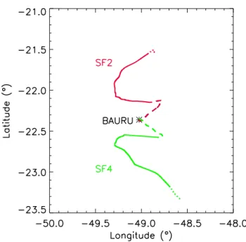
Fig. 1. Projection on the horizontal plan of the trajectory of the SF2
and SF4 balloon flights. The dashed, solid and dotted lines cor-respond respectively to the ascent, slow descent and rapid descent after cut down of the balloon. The red lines correspond to SF2 and green lines to SF4.
trajectories determined by this method are reliable providing that the modelled convective precipitation is well located.
Four sensitivity simulations were also run to test the im-pact on the results of the horizontal and vertical resolutions and of the microphysical scheme. The setup of theses simu-lations is explained in Sects. 4 and 5 together with the corre-sponding analysis of the results.
3.2 ECMWF analysis
The operational global analysis produced at ECMWF (Euro-pean Centre for Medium-range Weather Forecasts) are used in this study. One major characteristic of these analyses is that it includes the stratosphere up to the 1 hPa level. At the date of the HIBISCUS campaign, the ECMWF model had 60 vertical levels and a T511 truncation. ECMWF fields used are extracted on a 0.5◦
×0.5◦grid. The assimilation system
is a four-dimensional variational system including data over 12 h windows. For humidity, the data assimilated are the specific humidity profiles from radiosondes below 300 hPa, surface relative humidity and satellite radiances including moisture sensitivity. The longwave radiation parametriza-tion (Morcrette et al., 1998) is based on the Rapid Radiaparametriza-tion Transfer Model (Mlawer et al., 1997). It includes cloud ef-fects using maximum-random overlap of effective cloud lay-ers. The shortwave radiation scheme was originally devel-oped by Fouquart and Bonnel (1980) and revised by Mor-crette (1993). It takes into account the cloud properties for ice and liquid clouds.
4 Results for SF2 flight
4.1 SF2 flight and its meteorological environment
The SF2 balloon was launched from Bauru, State of S˜ao Paulo, Brazil (22.36◦S, 49.02◦W) at 20:18 UTC (18:18 local
summer time) on 13 February 2004. The balloon reached a maximum altitude of 20 km at sunset (22:11 UTC). Then the balloon experienced 3 h of slow night time descent down to 11.8 km where it was cut down. The trajectory of the balloon is shown in Fig. 1.
On 13 February 2004, the western and central parts of the State of S˜ao Paulo were located within the warm-sector ahead of a cold front advancing from Argentina, which reached South Brazil during the afternoon. During the af-ternoon of 13 February 2004, the Bauru radar observations showed that there was a moderate convective activity around Bauru with several weak convective cells developing within the radar range (240 km). At the time of the launch, there was a large area of instability moving in from north-west and west, but that never came closer than 300 km from the balloon track. It only reached Bauru around 07:00 UTC on 14 February, long after the end of the balloon flight. The meteorological situation is illustrated in Fig. 2a from the ac-cumulated rainfall estimated by the Tropical Rainfall Mea-suring Mission (TRMM, http://trmm.gsfc.nasa.gov) between 19:30 UTC on 13 February and 10:30 UTC on 14 February. More details on the meteorological situation can be found in Durry et al. (2006).
4.2 SF2 water vapour and temperature profiles
For the SF2 flight analysis, we make use of the H2O data
yielded by the micro-SDLA in the altitude region ranging from 18.5 km altitude after sunset (22:45 UTC) down to 4.6 km altitude (00:46 UTC) during its descent.
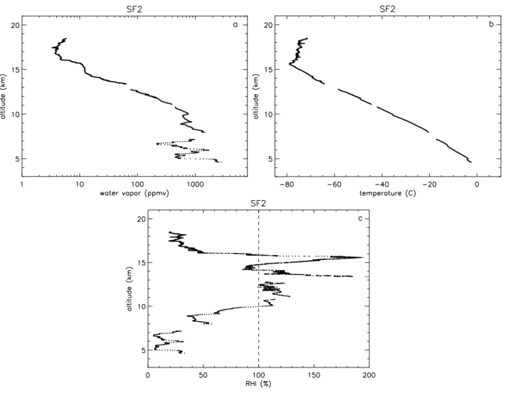
The water vapour mixing ratio (noted rvhereafter) and the
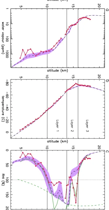
temperature profiles from micro-SDLA are shown in Figs. 3a and b. Note that there were no data between 12.774 and 13.385 km altitude because of technical problems. The wa-ter vapour profile (Fig. 3a) shows a large variability below 10 km altitude with a dry layer between 5 and 7 km. Above 10 km, there is a decrease with altitude up to an hygropause at 17 km altitude reaching ∼3 ppmv with enhanced variabil-ity between 14 and 17 km. Above 17 km, rvslowly increases
with altitude. The temperature (Fig. 3b) decreases with al-titude up to the cold point tropopause (−78.8◦C) at 15.5 km
altitude. Above 15.5 km, there is a large variability of the temperature profile with a tendency to slowly increase with altitude. Figure 3c depicts the relative humidity with respect to ice saturation in % (RHI) calculated from the measured temperatures and rv. To allow a fair comparison with the
model results (Sect. 5), the calculation of RHI is based on the formula of the saturation pressure with respect to ice used in the BRAMS model (Flatau et al., 1992) which provides
Fig. 2. Accumulated rainfall in mm (a) from TRMM between 19:30 UTC on 13 February 2004 and 10:30 UTC on 14 February 2004, (b)
from TRMM between 16:30 UTC on 24 February 2004 and 04:30 UTC on 25 February 2004, (c) from the reference run between 19:30 UTC on 13 February 2004 and 10:30 UTC on 14 February 2004, (d) from the reference run between 16:30 UTC on 24 February 2004 and 04:30 UTC on 25 February 2004. The green cross corresponds to the location of Bauru balloon launch site. The area plotted in these figures corresponds to the domain used in the BRAMS simulations.
RHI values close within +/−0.5% to those found using Son-ntag (1998)’s formula. The RHI profile shows that the air is very close to saturation or supersaturated between 10 and 16 km altitude. The very large supersaturation values up to RHI=190% are consistent with the water vapour data pre-sented in Ovarlez et al. (2000), Ovarlez et al. (2002) and Jensen et al. (2005a, b). The two layers where very large super-saturations occur (around 13.5 and around 15.5 km al-titude) are associated with enhanced water vapour mixing ra-tios. This indicates that, in these layers, the excess of water vapour has not been removed yet at the time of the measure-ments by ice nucleation and subsequent sedimentation of the condensed particles. Nevertheless, there are favourable con-ditions for the air to dehydrate within the following hours.
4.3 Comparison of the reference run and ECMWF analysis with SF2 measurements
The comparison between micro-SDLA SF2 measurements and the ECMWF analysis is shown in Fig. 4 and the com-parison between micro-SDLA SF2 measurements and the BRAMS reference run is shown in Fig. 5. The micro-SDLA data are averaged vertically in Fig. 4 (resp. Fig. 5) to match the ECMWF (resp. BRAMS reference run) vertical grid. To plot the ECMWF results, we have selected the profile the closest to the SF2 descent mean location plus the 8 profiles around from the 14 February 00:00 UTC analysis fields. To plot the BRAMS reference simulation results, we have se-lected the profile closest to the SF2 descent mean location plus all the profiles around as far as 60 km from this pro-file from hourly outputs between 22:00 UTC on 13 Febru-ary 2004 and 01:00 UTC on 14 FebruFebru-ary 2004. This time
Fig. 3. SF2 flight: (a) water vapour mixing ratio in ppmv from micro-SDLA measurements, (b) temperature in◦C from micro-SDLA
measurements, (c) derived relative humidity with respect to ice saturation (RHI) in %.
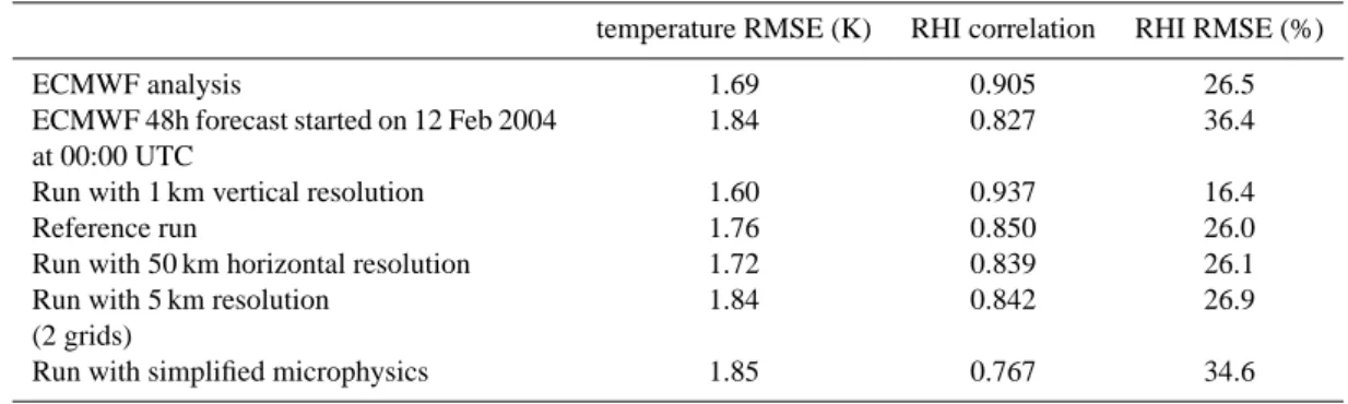
interval corresponds approximately to the descent duration. Note that in the 13–20 km layer where the BRAMS verti-cal resolution is 250 m (29 levels), there are only 8 ECMWF model levels corresponding to ∼1 km vertical spacing. Sta-tistical results comparing model and observations are given in Table 1. For the statistical analysis, RHI results were pre-ferred to rvresults to evaluate the water vapour model
per-formance since rv values cover several orders of magnitude
and therefore statistics for rvwould be weighted towards the
large rvat low altitudes. The other reason for this choice is
that RHI gives not only information on the water vapour but also on the state of the air parcel with respect to sub/super-saturation. The correlation for temperature is not given since it is greater than 0.999 for all model configurations.
Figures 4 and 5 show that the main water vapour and temperature features observed by micro-SDLA in the UTLS are largely smoothed when averaged on the ECMWF ver-tical grid while they are still present when averaged on the BRAMS reference run grid. ECMWF analysis does not
re-produce the observed variations in the UTLS. This is related to the vertical resolution which only allows the simulation of structures having a vertical extension greater than a few kilometres. Below 10 km, the ECMWF analysis exhibits a dry layer but moister than the mean microSDLA profile be-low 8 km. From 12 km upwards, ECMWF analysis generally underestimates rv, particularly above 15 km altitude. The
dry bias of the ECMWF analysis in the upper troposphere was already pointed out in several studies (e.g. Ovarlez and Van Velthoven, 1997; Ovarlez et al., 2000; Spichtinger et al., 2005). In the stratosphere, the ECMWF water vapour analy-sis field is nearly constant since no humidity data are avail-able for assimilation. For the temperature (Fig. 4b), there is a generally good agreement between micro-SDLA and the ECMWF analysis within 2 K. In particular, the ECMWF analysis exhibits a well-defined minimum of temperature at the cold point tropopause similar to micro-SDLA. In Fig. 4c, the ECMWF RHI profile shape is qualitatively similar to observations as illustrated by a RHI correlation of 0.905.
Table 1. Statistical results for SF2 flight: correlation and RMSE (Root Mean Square Error) between the model (ECMWF or BRAMS) and
micro-SDLA averaged over the corresponding model grid.
temperature RMSE (K) RHI correlation RHI RMSE (%) ECMWF analysis 1.69 0.905 26.5 ECMWF 48h forecast started on 12 Feb 2004
at 00:00 UTC
1.84 0.827 36.4
Run with 1 km vertical resolution 1.60 0.937 16.4
Reference run 1.76 0.850 26.0
Run with 50 km horizontal resolution 1.72 0.839 26.1 Run with 5 km resolution
(2 grids)
1.84 0.842 26.9
Run with simplified microphysics 1.85 0.767 34.6
Quantitatively, the ECMWF RHI is close to the observa-tions mainly below 10 km leading to 26.5% for the RMSE value. Note that there are no ECMWF RHI values greater than 100%. This illustrates the fact that supersaturated states with respect to ice are not allowed below a temperature of
−23◦C in the ECMWF model. Therefore, it is not possible
in the ECMWF analysis to reproduce the observed supersatu-rated layers in the UTLS. Moreover, because water vapour is removed instantaneously as condensed water below −23◦C
when superstaurated with respect to ice, the ECMWF analy-sis generally underestimates rvcompared to observations.
To make a fair comparison between results of the ECMWF analysis and of the BRAMS model, a sensitivity simulation was performed with a 1 km vertical resolution in the UTLS (∼ ECMWF vertical resolution) instead of the 250 m res-olution in the reference run. In Table 1 the statistical re-sults for the 1 km-resolution BRAMS simulation are calcu-lated using the micro-SDLA data averaged over the BRAMS 1km vertical grid. Results in Table 1 show that the sensitiv-ity run provides results for temperature similar to ECMWF analysis and a RHI mean profile (RHI RMSE=16.4%) sig-nificantly closer to the observations than ECMWF analysis (RHI RMSE=26.5%). This means that with a similar verti-cal resolution BRAMS performs similarly to ECMWF anal-ysis for temperature but significantly better for water vapour. Note that it is not pertinent to compare the statistics of the ECMWF analysis to those of the reference run since the for-mer (i) are calculated over a smaller number of points be-cause of the different vertical grid spacing used and (ii) cor-respond to an averaged profile in which the small scale struc-tures are largely smoothed.
As shown in Fig. 5, the vertical variations of rv,
tem-perature and RHI are generally reproduced in the BRAMS simulation although smoothed compared to the micro-SDLA measurements. The reference simulation provides the dry layer below 10 km altitude but not as dry as in the obser-vations, similarly to the ECMWF analysis. In this altitude range, the SF2 balloon was flown in a transition region
be-tween a dry and a moist air mass where the water vapour gradient is strong. The difference between the model and the observations indicates that the model dynamics has driven slightly too early the moist air mass associated to the front towards the Bauru area. The zigzag shape found in the obser-vations in this layer is also not reproduced by the mesoscale model. The small scale vertical variations in the observa-tions are likely due to sub-grid isolated convective cells cap-tured by the measurements but not by the model because of its spatial resolution. This hypothesis is supported by the fact that the backward trajectories crossed an area in which there were several small convective cells of a few kilometres horizontal extension in the Bauru radar observations. In the 10–14 km layer, the reference run shows a very good agree-ment with micro-SDLA measureagree-ments. In the 14–17.3 km range, the S-shape of the mean micro-SDLA profile is re-produced by the model but with less pronounced minima. Above 17.5 km altitude, the model gives nearly constant val-ues for rv with a low variability between the selected
pro-files as in ECMWF analysis. For temperature (see Fig. 5b), the reference simulation is generally in good agreement with the measurements (RMSE=1.76 K) except near the cold point tropopause level where the local sharp minimum is not sim-ulated by the model. There is a ∼5 K difference at 15.5 km altitude. As shown in Fig. 4b, this minimum is present in the ECMWF analysis. This important feature does not ap-pear in the ECMWF 48 h forecast started on 12 February at 00:00 UTC. It is brought in the 14 February 00:00 UTC analysis by the assimilation of observations. This indicates that the precursor information leading to this feature was not present in the 12 February 00:00 UTC ECMWF analy-sis used as initial state for the BRAMS simulations. More generally, the analysis gives better statistics than the forecast (see Table 1) thanks to data assimilation.
The general shape of the observed RHI profile in Fig. 5c is reproduced by the model (RHI correlation = 0.850 and RHI RMSE=26.0%) except around 15.5 km and 13.5 km al-titude where the model does not provide the observed large
Fig. 4. Comparison between ECMWF analysis and micro-SDLA
SF2 measurements (a) for water vapour in ppmv, (b) for tempera-ture in◦C and (c) for RHI in %. The micro-SDLA data are
aver-aged on the ECMWF model vertical grid and shown as a solid red line with the triangles showing the model levels. The black dashed line and the purple area show, respectively, the mean and the mini-mum/maximum for a set of selected model profiles. Details on the selected profiles are given in the text.
supersaturations and above 17.3 km where the model is sig-nificantly dryer. Unlike ECMWF analysis, BRAMS micro-physical scheme allows supersaturations with respect to ice at a given temperature. The threshold for the ice super-saturation in the model is 100% for the relative humidity
Fig. 5. Comparison between BRAMS reference simulation and
micro-SDLA SF2 measurements (a) for water vapour in ppmv, (b) for temperature in◦C and (c) for RHI in %. The micro-SDLA data
are averaged on the BRAMS model vertical grid and shown as a solid red line with the triangles showing the model levels. The black dashed line and the purple area show, respectively, the mean and the minimum/maximum for a set of selected model profiles. Details on the selected profiles are given in the text. In (c), the green solid line corresponds to RHI calculated using rvfrom the BRAMS reference
run and the micro-SDLA temperature. The green dashed line cor-responds to 100% saturation with respect to liquid water calculated using BRAMS mean temperature profile.
with respect to liquid water. This assumption is related to the BRAMS microphysical parameterization in which cloud
water mixing ratio is diagnosed using a test based on the satu-ration with respect to liquid water and the prognostic mixing ratios of total water, rain, cloud ice, aggregates, snow, grau-pel and hail (Walko et al., 1995). For the tropical UTLS con-ditions, this constraint (100% relative humidity with respect to liquid water) leads to large possible model ice supersatura-tions as illustrated in Fig. 5c (green dashed line). This means that the observed large ice supersaturations can be simulated by BRAMS leading to a slower removal of water vapour by ice nucleation than in the ECMWF model. This is illustrated by the generally greater values of rv simulated by BRAMS
in the 12–17 km layer compared to the ECMWF analysis leading to a better agreement with micro-SDLA. This indi-cates that there is a significant influence of the microphysical scheme on the water vapour mixing ratios in the upper tropo-sphere.
To test the importance of the horizontal resolution on the mesoscale model results two sensitivity tests were run. In the first one, we used a 50 km resolution (∼ECMWF horizontal resolution) in BRAMS instead of 20 km. The corresponding statistics that are given in Table 1 show that using a 50 km horizontal resolution leads to results very close to the refer-ence simulation. The second sensitivity simulation was run with two nested grids. The outer grid is the reference run grid (20 km horizontal resolution) and the inner grid is cen-tred on Bauru and has a 5 km horizontal resolution. For the 5 km grid, the convection parameterization is not used be-cause the convection parametrization is not designed for a 5 km grid and the convection can possibly be explicitly rep-resented with a 5 km grid. The statistics for this run are close to the reference run with a slight deterioration. The analysis of the two sensitivity runs shows the impact of the horizontal resolution is neutral. This indicates that, for this case study, the measured water vapour and temperature variations result mainly from the large scale dynamics rather than from local processes.
In summary, the mesoscale model performs better than ECMWF analysis in predicting the observed SF2 water vapour and RHI profiles when run with a similar resolution. With a 250 m vertical resolution, the BRAMS model is able to simulate most of the observed small scale vertical varia-tions thanks to the fine vertical resolution and to a realistic representation of the microphysical processes. In this case, a fine vertical resolution is more important than a fine hor-izontal resolution because the observed variations of water vapour are mainly linked to the large scale dynamics. 4.4 Analysis of the reference run for SF2
In this section, we analyse the model results in order to iden-tify the processes leading to the modelled temperature and humidity profiles and to understand the model behaviour compared to the observations. This study being focused on the UTLS we will restrict this analysis to the results above 10 km altitude. Within the UTLS (meaning here above
10 km) it is possible to identify the TTL (tropical tropopause layer) which is the transitional layer between air with tro-pospheric properties and air with stratospheric properties (Highwood and Hoskins, 1998; Folkins et al., 1999). The issue of how to define the TTL is not settled. Here, we define the top at the lapse rate tropopause (WMO defini-tion) and the bottom where the lapse rate (−∂T /∂z) starts departing from typical tropospheric values (7–8 K km−1)
to-wards stratospheric values (negative values). Using this def-inition we found that the model predicts a TTL extending from 13.7 to 15.9 km. This result is compared to the TTL extension determined by Durry et al. (2006) from the SF2 micro-SDLA temperatures and the quasi-simultaneous ozone sounding measurements. They found using the chemopause for the bottom of the TLL and the lapse rate tropopause for the top that the observed TTL is between 13.5 and 15.5 km altitude. Thus, the TTL predicted by the model is in agree-ment within 0.4 km with micro-SDLA measureagree-ments. But the model does not provide the observed sharp temperature minimum around 15.5 km but a fairly smooth transition be-tween the positive and the negative lapse rates.
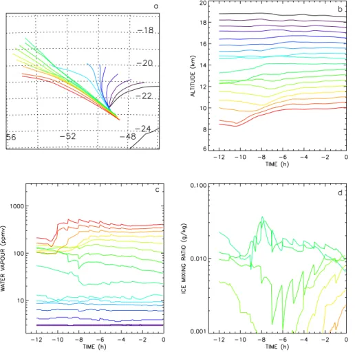
A trajectory analysis is used to diagnose the processes that lead to the modelled water vapour and temperature profiles above 10 km altitude. Backward trajectories were calculated along the SF2 descent locations using the methodology pro-posed by Freitas et al. (2000). The trajectories are only reli-able if the modelled convective precipitation is well located. This point is checked by comparing the TRMM accumulated rainrate (Fig. 2a) to the model accumulated rainrate (Fig. 2c). The comparison shows that, although the model simulates significantly less precipitation amount than observed, the spatial pattern of the model precipitation field agrees gener-ally well with the TRMM observations. Only backward tra-jectories over 12 h are used since the analysis performed here is limited to the processes that occur just before the flight measurements.
Three layers are defined in this analysis: layer 1 corre-sponding to tropospheric air below the TTL base, layer 2 cor-responding to the TTL and layer 3 corcor-responding to strato-spheric air above the TTL top. The results of the trajectory analysis are given in Fig. 6 and summarized in Table 2. In layer 1 (10–13.7 km), the model predicts very accurately both temperature and RHI profiles except for the thin layer of su-persaturated air observed in the 13.5–14 km altitude range (Fig. 5c). This particular layer will be discussed in more de-tails below together with the analysis of layer 2. Between 10 and 12.8 km, the model results agree very well for the temperature and for rv and thus for RHI. In this layer, the
trajectory analysis indicates that the air is lifted by the front located south-west of Bauru and experiences the formation of large amounts of ice particles leading to a significant removal of water vapour (dehydration). This shows that the model is able to simulate well both the dynamical and the microphys-ical processes that lead to the observed rvand T. To test the
Fig. 6. Results from the 12-h backward trajectories calculated using the reference run results for SF2. (a) Map of the trajectories, (b) Altitude
in km as a function of time in h, (c) water vapour mixing ratio in ppmv as a function of time in h and (d) ice (cloud+precipitation) mixing ratio in g kg−1as a function of time in h.
Table 2. Characteristics of the three layers identified from the SF2 trajectory analysis based on the BRAMS reference simulation above
10 km altitude.
Altitude range (km) Air mass origin vert./horiz.
Moisture tendency
Ice condensation during previous hours Layer 1 10–13.7 Mid and upper troposphere below the
TTL/South-west
drying yes
Layer 2 (TTL) 13.7–15.9 Upper troposphere below the TTL and TTL /South-west
drying below 14.3 km and
constant above
yes only below 14.3 km
Layer 3 Above 15.9 Stratosphere/South changing to East with increasing altitude
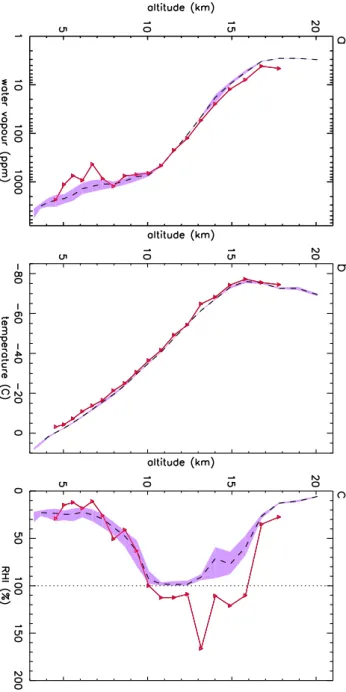
constant No
sensitivity simulation was run with simplified microphysics in which the water vapour can only be condensed as liquid cloud water where supersaturation with respect to liquid wa-ter occurs (i.e. no ice particles can be produced). For the sensitivity run displayed in Fig. 7, rvmean profile in layer 1
is greater by about a factor of 1.4 on average compared to the reference run. This is confirmed by the statistical results given in Table 1. This large difference comes from the ice formation/growth and the consecutive dehydration by sedi-mentation which are not taken into account in the simplified
microphysics run. This indicates that it is necessary to in-clude this process to obtain a realistic water vapour profile.
In layer 2 (TTL, 13.7–15.9 km), the trajectory analysis showed that the air slowly rises due to radiative warming except below 14.3 km where there is some formation of ice because of air ascent during the previous 12 h leading to de-hydration. At the time of the flight, the 13.5–14.3 km layer in the model is still slightly supersaturated and the water vapour mixing ratio is nearly constant in the model during the 6 h preceding the flight. This quasi steady-state is ex-plained by the fact that the decrease of rvdue to ice
conden-sation leads to an increase of temperature through latent heat release which restricts the supersaturation and thus the de-crease of rvdue to the ice formation. The large peaks of
su-persaturation observed around 13.5 km and around 15.5 km (Fig. 5c) are not reproduced by the model which produces too warm temperatures (Fig. 5b) at these altitudes. The wa-ter vapour field being linked to temperature conditions in par-ticular when close to saturated conditions, it is important to evaluate the possible impact of the model temperature over-estimation on the water vapour field. For this purpose, RHI was recalculated using the model rv profile and the
micro-SDLA temperatures instead of the model temperatures. The result displayed in Fig. 5c (green solid line) shows that if the BRAMS model had simulated more realistic temperatures in these two layers it would have lead to larger ice supersatura-tions and thus to a much better agreement with micro-SDLA RHI profile, particularly for the layer around 15.5 km alti-tude. This is also shown by the RHI RMSE calculated for the reference run but with the measured temperatures which is largely improved: 15.7%.
In the lower stratosphere (layer 3, above 15.9 km), the BRAMS model predicts a temperature consistent with the micro-SDLA measurements. The rv profile is slightly
moister below 17.2 km and largely drier above. The trajec-tory analysis shows that, in layer 3, there is no ice forma-tion because the air does not experience saturated or super-saturated conditions during the past 12 h. Above 17.2 km, the model produces a stratospheric water vapour profile very close to the ECMWF analysis. This is because no small or meso-scale processes occur. Indeed, the water vapour distri-bution in this layer is mainly driven by the large scale hori-zontal fluxes since (i) vertical motions are weak and there is no convective overshooting in the BRAMS domain and (ii) no microphysical processes occur because air is largely un-dersaturated.
In summary, simulation results showed that the micro-physical processes play an important role in the distribution of water vapour and an appropriate parameterization allow-ing supersaturation with respect to ice is needed to model the observed rvprofiles. In near saturated or supersaturated
lay-ers it is necessary to simulate realistic temperatures since mi-crophysical processes are extremely temperature dependent.
Fig. 7. Same as Fig. 5 but for the BRAMS sensitivity run with
simplified microphysics (see text for details on this run).
5 Results for SF4 flight
5.1 SF4 flight and its meteorological environment
The SF4 balloon was launched from Bauru at 20:03 UTC on 24 February 2004. The balloon reached a maximum al-titude of 20.2 km shortly before sunset followed by 45 min float and a slow descent (starting at 21:57 UTC) down to 10.7 km where it was cut down (00:17 UTC). The trajectory of the balloon is shown in Fig. 1.
Fig. 8. Same as Fig. 3 but for SF4 flight measurements.
From noon onwards, a massive complex convective sys-tem was heading towards Bauru. At the time of the launch, the system was about 120 km north-west of Bauru, moving at 40 km h−1south-eastwards. It reached Bauru shortly after
20:00 UTC. This system was part of a very large area of con-vection (SACZ; South Atlantic Convergence Zone) covering the State of S˜ao Paulo and extending over the ocean. The situation is illustrated in Fig. 2b by the accumulated TRMM rainfall between 24 February at 16:30 UTC and 25 February at 04:30 UTC. A more complete description of the meteoro-logical situation is given in Durry et al. (2006).
5.2 SF4 water vapour and temperature profiles
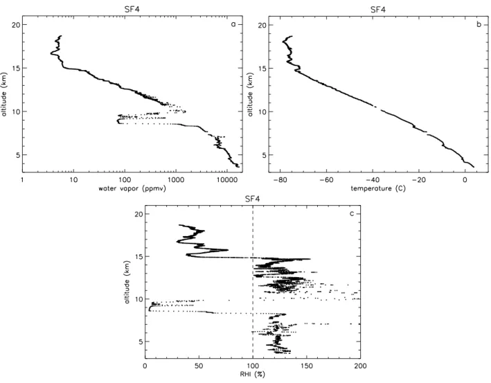
For the SF4 flight analysis, we use H2O data achieved during
the descent of the sensor in the altitude region ranging from 18.7 km (24 February at 22:21 UTC) down to 3.6 km (25 February at 00:48 UTC). rv, temperature and RHI profiles
for the SF4 flight are shown in Fig. 8. One important feature in Fig. 8a is a very dry layer around 9 km with mixing ratios
below 100 ppmv. The rvprofile also exhibits relative minima
of water vapour around 15 km and 16.7 km altitude. The tem-perature profile decreases fairly monotonically up to 14.5 km altitude. Above there are significant variations with altitude with an absolute minimum of −78.8◦C at 18.1 km. The
mea-sured profile is supersaturated up to 15 km altitude with the exception of the very dry layer between 8.5 and 10 km (see Fig. 8c). In this very dry layer, RHI reaches values below 10%. Typical supersaturations are around RHI=125% with peaks up to 195%. Note that the water vapour profiles and the temperature profiles above 15 km for the SF2 and SF4 flights are significantly different. This is related to the differ-ent meteorological conditions in which the two profiles were measured.
5.3 Comparison of the reference run and ECMWF analysis with SF4 measurements
For SF4, the comparison between micro-SDLA and the ECMWF analysis (resp. reference run) is displayed in Fig. 9
Fig. 9. Same as Fig. 4 but for SF4.
(resp. Fig. 10). We used ECMWF analysis at 00:00 UTC on 25 February 2004 and BRAMS hourly outputs from 22:00 UTC on 24 February 2004 to 01:00 UTC on 25 Febru-ary 2004.
Figure 9a shows that ECMWF analysis rv is generally
dryer than the micro-SDLA rv mean profile for all altitudes
except in the very dry layer located around 9 km which is well captured by the ECMWF analysis. For temperature (Fig. 9b), the ECMWF analysis is consistent with the mi-croSDLA measurements within 1 K. The ECMWF RHI pro-file (Fig. 9c) reproduces the general shape of the observations (RHI correlation=0.801) but is characterised by largely lower
Fig. 10. Same as Fig. 5 but for SF4.
values (RMSE=48.5%) compared to microSDLA RHI ex-cept in the dry layer (see Table 3). There is hardly any super-saturation with respect to ice in the ECMWF analysis in the layers 3.5–8 km and 10–15 km. As for SF2, ECMWF anal-ysis underestimates water vapour in the upper troposphere (above 10 km). This is partly because water vapour is imme-diately converted into ice when supersaturation with respect to ice occurs below −23◦C. Another reason for the poor
ac-curacy of ECMWF water vapour analysis in the UTLS is the few humidity data that are used in the assimilation system. Nevertheless, ECMWF analysis (14 February 00:00 UTC) is better than the 48 h forecast started on 12 February at 00:00 UTC as illustrated by the statistics given in Table 3.
Fig. 11. Same as Fig. 6 but for SF4.
Table 3. Same as Table 1 but for SF4 flight.
temperature RMSE (K) RHI correlation RHI RMSE (%) ECMWF analysis 0.80 0.801 48.5
ECMWF 48 h forecast started on 23 Feb 2004 at 00:00 UTC
1.15 0.615 63.7
Run with 1 km vertical resolution 1.19 0.716 38.4
Reference run 1.26 0.778 33.9
Run with 50km horizontal resolution 1.29 0.769 35.1 Run with 5 km resolution
(2 grids)
1.45 0.748 37.1
Run with simplified microphysics 1.63 0.499 54.9
As previously done for SF2, a sensitivity test with BRAMS was performed using a 1 km vertical resolution sim-ilar to the ECMWF model to allow a possible comparison to the ECMWF analysis. The corresponding results are given in Table 3. When using a 1 km vertical resolution, the BRAMS simulation RHI profile is significantly closer to
the observations (RMSE=38.4%) than the ECMWF analysis (RMSE=48.5%). This is the contrary for temperature with values of RMSE of 1.19 K for the BRAMS and 0.80 K for ECMWF analysis. This means that for SF4, the ECMWF analysis is better for temperature compared to BRAMS with a similar vertical resolution. In Table 3 are also given the
statistics for the ECMWF 48 h forecast started on 23 Febru-ary 2004, i.e. having the same initial state as the BRAMS simulations. Temperature RMSE for the ECMWF 48 h fore-cast is similar to the mesoscale simulation with 1km vertical resolution. This indicates that the good performance of the ECMWF analysis for temperature comes from the data as-similation. For RHI, the analysis statistics are poor but better than the 48h forecast statistics also thanks to data assimila-tion.
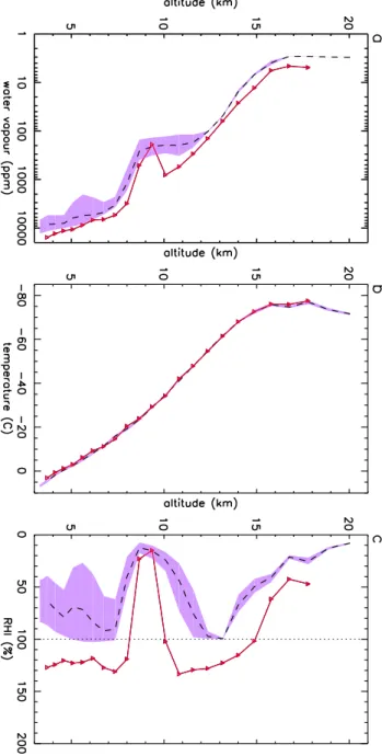
As shown in Figs. 10a and b, the main water vapour and temperature variations observed by micro-SDLA in the UTLS (TTL) are kept when averaged on the BRAMS ref-erence run grid. The model profiles reproduce the general patterns found in the observations but they are smoother. In Fig. 10a, the mesoscale model produces a dry layer around 10 km altitude but significantly too moist compared to the micro-SDLA observations and the ECMWF analysis and lo-cated about 1 km higher. In the reference run, the SF4 flight track at the altitude of the dry layer is located in a transi-tion zone associated with a large rvgradient as illustrated by
the large variability of the selected model profiles around the SF4 flight track in this layer. This transition zone is oriented north-west/south-east and located between the moist convec-tion zone south of the transiconvec-tion zone and the dry intrusion of low stratosphere mid-latitude air (∼100 ppmv) north of the transition zone as analysed by Durry et al. (2006). In the ECMWF analysis the SF4 flight track is located within the dry intrusion and gives more realistic results for the dry layer. This can be explained by the fact that for SF4: (i) the data as-similation has significantly decreased the water vapour mix-ing ratio in this layer and (2) the whole ECMWF analysis profile is significantly dryer than the observations. The com-parison between the reference simulation and the microS-DLA measurements indicates that the reference simulation forecasts the dry intrusion too far from the SF4 flight loca-tion, shifted by about 150 km. Below this layer, the reference run rv profile is dryer than micro-SDLA. Above 12 km the
model rvis consistent with the measurements up to 16.8 km
altitude. The micro-SDLA step-function shape is reproduced by the model although shifted in altitude by about 0.5 km. Above 16.8 km, the model is significantly dryer than the ob-servations and exhibits very limited variations. Figure 10b shows that the temperature is well simulated in the refer-ence run (RMSE=1.26 K) although the fine scale variations between 14.7 and 18 km are not produced by the model. For RHI (Fig. 10c), the model reproduces the general shape (RHI correlation=0.778) with generally significantly lower values (RMSE for RHI=33.9%).
The importance of the horizontal resolution is evaluated using two test simulations with 50 km and 5 km horizontal resolutions. Results of these sensitivity tests are fairly similar to the reference simulation as shown by the statistics given in Table 3. Similarly to SF2, there is no improvement possibly because the water vapour profile is mainly driven by the large scale dynamics.
In summary, the ECMWF analysis and the BRAMS sim-ulations give good results for temperature and significantly underestimate on average RHI although the BRAMS model performs better. Compared to SF2, SF4 statistical results are slightly better for temperature (∼1.2 K RMSE for SF4 and
∼1.7 K for SF2) but worse for RHI (∼35% RMSE for SF4
and ∼25% for SF2) and consequently for rv. This indicates
that the BRAMS water vapour performance depends on the considered meteorological situation.
5.4 Analysis of the reference run for SF4
In this section we analyse in more details the BRAMS model behaviour compared to observations in the UTLS (above 10 km). The TTL base and top altitudes derived from the reference run are 14.2 and 16.6 km. The TTL characteris-tics derived from micro-SDLA data by Durry et al. (2006) are 13.3 km for the base and 17.8 km for the top. There-fore, the model predicts a TTL thinner than observed. In the micro-SDLA observations, there is a layer between ∼16.8 and ∼17.7 km altitude where the water mixing ratio is high (∼5 ppmv) and the temperature tendency is negative. From the analysis of complementary ozone and CH4 data, Durry
et al. (2006) suggested that this layer had been moistened and cooled adiabatically by a convective transport that had occurred a few days before the flight. This moist and cold layer is not captured by the model leading to a TTL top at a lower altitude in the model. The 0.9 km difference between the TTL base observed and modelled may be attributed to the TTL base definitions used: the chemopause for the observa-tions and the lapse rate for the model.
As for SF2, 12-h backward trajectories were calculated from the reference run outputs at the location of the SF4 flight. The modelled precipitation (Fig. 2d) is less in amount than the satellite observations but it is well located as illus-trated by the comparison with TRMM accumulated rainrate (Fig. 2b). The results of the trajectory calculation are shown in Fig. 11 and summarized in Table 4. As for SF2, we define three layers: layer 1 below the TTL (10–14.2 km), layer 2 being the TTL (14.2–16.6 km) and layer 3 being the lower stratosphere (above 16.6 km). In layer 1 (10–14.2 km), the reference run rv and RHI are underestimated by the model
mainly below 11km. The 10–11 km layer is the transition be-tween the very dry layer and a moist layer. The model fails to reproduce the observed very sharp transition related to the intrusion of stratospheric extratropical air which started a few days before the flight. This intrusion has likely been smoothed during the two preceding days in the model by the turbulent mixing parametrization. This hypothesis is sup-ported by the calculation of rvintegrated over the layer where
the model predicts the dry intrusion (8.3 and 11.3 km) giving a 5% difference between micro-SDLA and the model results. This means that there is approximately the same amount of water vapour in the dry intrusion layer in the observations and in the model but it is more diluted in the model. The air
Table 4. Same as Table 2 but for SF4.
Altitude range (km) Air mass origin vertical/horizontal
Moisture tendency
Ice condensation during previous hours
Layer 1 10–14.2 Mid and upper troposphere below the TTL/North-west
Moistening below 12.6 km and drying above
Yes above 11 km and increasing with altitude
Layer 2 (TTL) 14.2–16.6 TTL/North-west changing to North with increasing altitude
Constant No
Layer 3 Above 16.6 Stratosphere/North changing to East with increasing altitude
Constant No
mass sampled by SF4 in layer 1 comes from ascending air from lower levels leading to a moistening during the hours preceding the flight. This moistening effect related to the dy-namics competes with the removal of water vapour by ice nu-cleation and subsequent ice growth and sedimentation. This microphysical process becomes dominant in the model above 12.6 km leading to a net decrease of water vapour mixing ratio. The analysis of the SF2 flight showed that the tem-perature errors in the BRAMS simulation have an impact on the model’s ability to reproduce the water vapour observa-tions. For SF4, the temperature error is weaker (Fig. 10b and Table 3) and its impact is only important in the 12.5– 14.7 km layer as illustrated in Fig. 10c (green solid line). In this layer, using the micro-SDLA temperature measurements and the BRAMS rv to calculate RHI leads to an increase of
RHI consistent with the observations. This result shows that part of the RHI underestimation in layer 1 is due to temper-ature errors in the model. The complementary possible ex-planations are an insufficient moistening of this layer by air ascent and/or a too fast drying by ice formation.
In layer 2 (TTL, 14.2–16.6 km), the water vapour does not exhibit significant changes during the preceding hours since it does not experience significant uplifting or ice formation because of undersaturated conditions. The distribution of water vapour in the TTL depends on the dynamics. Below 15.2 km the trajectory analysis shows that the air originates from a relatively dry area located north-west of the flight track. In the 14.2–15.2 km layer, the BRAMS model is able to reproduce the observed shape and values for rv and RHI.
Between 15.2 and 16.6 km the air comes from the convec-tive area north of Bauru. This air is undersaturated within the 12 h preceding the flight but it is more humid in terms of relative humidity than below because previously moist-ened by convection (see Figs. 2b and d). This effect becomes less important above 16 km altitude leading to the decrease of the BRAMS RHI between 16 and 16.6 km. Nevertheless, the BRAMS model is able to simulate the observed varia-tions of rvand RHI between 14.2 and 16.6 km meaning that
the model dynamics is realistic and in particular the location of the convection. Above 16.6 km in the lower stratosphere
(layer 3), the model water vapour variations are small lead-ing to a negligible impact of the horizontal dynamics on the water vapour distribution. As for SF2, the BRAMS model initial state for rvis fairly homogeneous above 17 km. The
rvfield is not changed during the simulation since this layer
is not affected by any air ascent or ice nucleation.
6 Conclusion
The objective of this paper is to evaluate the ability of the BRAMS mesoscale model to simulate the observed vertical variations of water vapour in the tropical UTLS. This eval-uation is based on comparisons with in situ water vapour and temperature measurements but also comparisons with ECMWF analysis fields in order to show the potential ben-efits of a mesoscale model with respect to a global analysis. The water vapour and temperature measurements were gath-ered by the micro-SDLA instrument during the SF2 and SF4 HIBISCUS balloon flights. Both flights exhibit large varia-tions of water vapour in the UTLS but also large differences are found between the two sets of measurements. In both flights, layers with large supersaturations with respect to ice are observed.
The measured fine scale vertical structures in the UTLS have a typical length of 1 km or less. This is why a 250 m vertical grid-spacing was used in the UTLS in the BRAMS. The ECMWF model having a ∼1 km vertical grid-spacing in the UTLS can only give a smooth picture of the observed variations of temperature and water vapour. Apart from the vertical resolution, the differences between the BRAMS ref-erence simulation and the ECMWF analysis are:
– the horizontal resolution: 20 km for BRAMS and
∼50 km for ECMWF,
– a more complete microphysical scheme in BRAMS
giv-ing the possibility of large supersaturations with respect to ice,
– the assimilation of data in the ECMWF analysis when
valuable recent meteorological information leading to an update of the atmospheric state compared to any forecast (from BRAMS or ECMWF).
Sensitivity simulations with BRAMS were run to evaluate the impact of the vertical resolution, horizontal resolution and microphysical scheme on the mesoscale model perfor-mances.
The analysis of the results showed that the ECMWF anal-ysis performs well compared to the micro-SDLA measure-ments for temperature for both flights. This is related to the data assimilation system which improves significantly the temperature field. As already found in previous studies (e.g. Ovarlez et al., 2000), we showed that ECMWF analy-sis generally underestimates water vapour in the upper tro-posphere. In supersaturated layers, we pointed out that the microphysical scheme removes instantaneously the excess of water vapour with respect to ice leading to lower water vapour mixing ratios compared to observations. Very re-cently, Tompkins et al. (2005) tested a new parameterization that attempts to represent ice supersaturation and the homo-geneous ice nucleation process in the ECMWF model. They showed that this new parameterization leads to a reduction of the upper troposphere dry bias. In undersaturated conditions below 10 km altitude, ECMWF analysis reproduces gener-ally well micro-SDLA water vapour profile. This is because water vapour information from radiosoundings below 10 km is used in the assimilation system. This is also because in undersaturated conditions the water vapour distribution does not rely on the microphysics but depends on the dynamics that is also well constrained by data assimilation. Above 17 km altitude, ECMWF analysis is drier than micro-SDLA for both flights.
The mesoscale simulation with the BRAMS model pro-vides a generally good estimation of the measured temper-ature profiles except in layers with large gradients or with small scale variations of the gradient which are not well cap-tured. In particular, this leads to a difference of ∼5 K at the cold point tropopause between micro-SDLA and BRAMS for SF2. For SF4, the BRAMS statistical results for tempera-ture are slightly worse than the ECMWF analysis but similar to the ECMWF 48 h forecast.
For water vapour and RHI (relative humidity with respect to ice saturation), the BRAMS model with a 1 km vertical resolution gives significantly better results than the ECMWF analysis with a reduction of the RHI RMSE of about 10% in both cases. This improvement is mainly due to the mi-crophysical scheme in BRAMS which can give ice supersat-urations and a progressive removal of water vapour by ice nucleation and subsequent growth and sedimentation. The mesoscale simulation with a 250 m vertical resolution is able to reproduce most of the observed vertical variations of water vapour and of RHI. Neverthess, it does not exhibit very large ice supersaturations (max RHI ∼130%) like those found in the micro-SDLA data (max RHI>150%). This can be
ex-plained by the fact that (i) measured highest supersaturations are likely to be a transient state just before ice nucleation occurs and (ii) the BRAMS microphysical scheme is a bulk type parameterization which is less precise than a spectral bin parameterization for thin cirrus simulation as shown by Khvorostyanov et al. (2006). The impact of the horizontal resolution is small for both case studies. Above 17 km al-titude, the underestimation of water vapour by BRAMS is similar to the ECMWF analysis since no mesoscale process affects the lower stratosphere in the BRAMS simulations.
From a trajectory analysis, it was shown that the water vapour variations in the model depend on the dynamical and thermodynamic processes experienced by the sampled air parcel. The profiles from two flights undergo a range of different dynamical processes: uplifting from the mid tro-posphere, large scale transport associated with a front, isen-tropic transport from the mid-latitude upper troposphere and convection. The dynamical processes are dominant in un-dersaturated conditions. In near-saturated or supersaturated conditions the thermodynamic environment, i.e. the air tem-perature, plays a major role since it controls the ice nu-cleation process and consequently the dehydration. For in-stance, the sharp minimum of temperature at the cold point tropopause in SF2 is not captured by the model leading to a large underestimation of RHI. In supersaturated layers where the BRAMS temperature is close to micro-SDLA, the model water vapour profile is generally close to the observations showing the good quality of the model’s microphysical pa-rameterization. The origin of the temperature uncertainties found in the BRAMS simulations and the ECMWF forecasts were not investigated in the present study. Temperature be-ing dependent on many processes (radiative, dynamic, ther-modynamic and microphysical), a special work needs to be done on this issue.
The BRAMS mesoscale model is able to reproduce most of the vertical variations of water vapour in the UTLS. But the two cases studied in this paper are not sufficient to fully evaluate the mesoscale model performances to simulate the UTLS water vapour. In particular, since only one measured profile was available per case study, it was not possible to fol-low the time evolution of the water vapour structures. This knowledge of the time evolution would help confirming our interpretation of the processes involved in the variations of water vapour. A larger set of data was acquired during the SCOUT-AMMA field experiment that took place in west-ern Africa in 2006. This will give the opportunity to obtain a more complete description from observations of the time evolution of the dynamical, thermodynamic and microphysi-cal processes driving the UTLS water vapour. Also the avail-ability of more accurate water vapour sensors in radiosound-ing systems will be a determinant tool in the understandradiosound-ing of the water vapour evolution in the UTLS.
Acknowledgements. This modelling study is supported by funds
contract EVK2-2001-000111) and the French Centre National de la Recherche Scientifique (Programme National de Chimie Atmosph´erique). This work makes use of the RAMS model, which was developed under the support of the National Science Foundation (NSF) and the Army Research Office (ARO). BRAMS model development and maintenance is supported by Brazilian Funding Agency for Studies and Projects (FINEP). Computer ressources were provided by CINES (Centre Informatique National de l’Enseignement Sup´erieur), project pce2227. The TRMM data were provided by GSFC/DAAC, NASA. The authors thank the coordinators of the TroCCiBras Project and the personnel of the Meteorological Research Institute (IPMet) of the S˜ao Paulo State University (UNESP) for providing the infrastructure support during the campaign and the personnel of the Centre National d’Etudes Spatiales (CNES) for their support in balloon, radar and sondes operations. We acknowledge G. Held of IPMet for providing the Bauru radar observations and assisting with their interpretation.
Edited by: P. Haynes
References
Brewer, A. W.: Evidence for a world circulation provided by mea-surements of helium and water vapour distribution in the strato-sphere, Quart. J. Roy. Meteorol. Soc., 75, 351–363, 1949. Durry, G. and M´egie, G.: Atmospheric CH4 and H2O
monitor-ing with near-infrared InGaAs laser diodes by the SDLA, a bal-loonborne spectrometer for tropospheric and stratospheric in situ measurements, Appl. Opt., 38, 7342–7354, 1999.
Durry, G. and Megie, G. : In situ measurements of H2O from a stratospheric balloon by diode laser direct-differential absorption spectroscopy at 1.39 µm, Appl. Opt., 39, 5601–5608, 2000. Durry, G., Hauchecorne, A., Ovarlez, J., Ovarlez, H., Pouchet, I.,
Zeninari, V., and Parvitte, B.: In situ measurement of H2O and CH4 with telecommunication laser diodes in the lower strato-sphere: dehydration and indication of a tropical air intrusion at mid-latitudes, J. Atmos. Chem., 43, 175–194, 2002.
Durry, G., Amarouche, N., Z´eninari, V., Parvitte, B., Le Barbu, T., and Ovarlez, J.: In situ sensing of the middle atmosphere with balloonborne near-infrared laser diodes, Spectrochimica Acta, Part A, 60, 3371–3379, 2004.
Durry, G. and Hauchecorne, A.: Evidence for long-lived polar vor-tex air in the mid-latitude summer stratosphere from in situ laser diode CH4 and H2O measurements, Atmos. Chem. Phys., 5, 1467–1472, 2005,
http://www.atmos-chem-phys.net/5/1467/2005/.
Durry, G., Zeninari, V., Parvitte, B., Le Barbu, T., Lefevre, F., Ovar-lez, J., and Gamache, R. R.: Pressure-broadening coefficients and line strengths of H2O near 1.39 µm: application to the in situ sensing of the middle atmosphere with balloonborne diode lasers, J. Quant. Spectrosc. Radiat. Trans., 94(3–4), 387–403, 2005.
Durry, G., Huret, N., Hauchecorne, A., et al.: Isentropic advection and convective lifting of water vapor in the UT-LS as observed over Brazil (22◦S) in February 2004 by in situ high resolution
measurements of H2O, CH4, O3 and temperature, Atmos. Chem. Phys. Discuss., 6, 12 469–12 501, 2006.
Flatau, P. J., Walko, R. L., and Cotton, W. R.: Polynomial fits to saturation vapour pressure, J. Appl. Meterorol., 31, 1507–1513,
1992.
Folkins, I., Loewenstein, M., Podolske, J., Oltmans, S., and Proffitt, M.: A barrier to vertical mixing at 14 km in the tropics: Evidence from ozonesondes and aircraft measurements, J. Geophys. Res., 104, 22 095–22 102, 1999.
Fouquart, Y. and Bonnel, B., Computations of solar heating of the earth’s atmosphere: a new parametrization, Breitr. Phus. Atmo-sph., 53, 35–62, 1980.
Freitas, S. R., Silva Dias, M. A. F., Silva Dias, P. L., Longo, K. M., Artaxo, P., Andreae, M. O., and Fischer, H.: A convective kine-matic trajectory technique for low-resolution atmospheric mod-els, J. Geophys. Res., 105, 24 375–24 386, 2000.
Freitas, S., Longo, K., Silva Dias, M., Silva Dias, P., Chatfield, R., Prins, E., Artaxo, P., Grell G., and Recuero, F.: Mon-itoring the transport of biomass burning emissions in South America. Environmental Fluid Mechanics, 5(1–2), 135–167, doi:10.1007/s10652-005-0243-7, 2005.
Fueglistaler, S., Wernli, H., and Peter, T.: Tropical troposphere-to-stratosphere exchange inferred from trajectory calculations, J. Geophys. Res., 109, D03108, doi:10.1029/2003JD004069, 2004. Fujiwara, M., Shiotani, M., Hasebe, F., V¨omel, H., Oltmans, S., Ruppert, P. W., Horinouchi, T., and Tsuda T.: Performance of the meteolabor “Snow White” chilled-mirror hygrometer in the tropical troposphere: Comparisons with the Vaisala RS80 A/H-Humicap sensors, J. Atmos. Ocean. Technol., 20, 1534–1542, 2003.
Gettelman, A., Randel, W. J., Wu, F., and Massie, S. T.: Transport of water vapour in the tropical tropopause layer, Geophys. Res. Lett., 29, 1009, doi:10.1029/2001GL013818, 2002.
Gevaerd, R. and Freitas, S.: Estimativa operacional da umidade do solo para iniciao de modelos de previso numrica da atmosfera. Parte 1: descrio da metodologia e validao, Brazilian J. Meteorol., LBA Special Issue, 21, 3a, 59–73, 2006.
Grell, G. A. and Devenyi, D.: A generalized approach to parameterizing convection combining ensemble and data assimilation techniques, Geophys. Res. Lett., 29, 1693, doi:10.1029/2002GL015311, 2002.
Harrington, J. Y.: The effects of radiative and microphysical pro-cesses on simulated warm and transition season Arctic stratus, PhD Diss., Atmospheric Science Paper No. 637, Colorado State University, Department of Atmospheric Science, Fort Collins, CO 80523, 289 pp, 1997.
Hatsushika, H. and Yamazaki, K.: Stratospheric drain over Indone-sia and dehydration within the tropical tropopause layer diag-nosed by air parcel trajectories, J. Geophys., Res., 108, D4610, doi:10.1029/2002D002986, 2003.
Highwood, E. J. and Hoskins, B. J.: The tropical tropopause, Quart. J. Roy. Meteorol. Soc., 124, 1579–1604, 1998.
Hintsa, E., Weinstock, E. M., Anderson, J. G., May, R. D., and Hurst, D. F.: On the accuracy of in situ water vapour measure-ments in the troposphere and lower stratosphere with the Harvard Lyman-a hygrometer, J. Geophys. Res., 104, 8183–8190, 1999. Holton, J. R., Haynes, P. H., McIntyre, M. E., Douglass, A. R.,
Tood, R. B., and Pfster, L.: Stratosphere-troposphere exchange, Rev. Geophys., 105, 1879–1888, 1995.
Jensen, E. and Pfister, L.:Transport and freeze-drying in the tropical tropopause layer, J. Geophys. Res., 108, D02207, doi:10.1029/2003JD004022, 2004.