HAL Id: inria-00602500
https://hal.inria.fr/inria-00602500
Submitted on 22 Jun 2011
HAL is a multi-disciplinary open access
archive for the deposit and dissemination of
sci-entific research documents, whether they are
pub-lished or not. The documents may come from
L’archive ouverte pluridisciplinaire HAL, est
destinée au dépôt et à la diffusion de documents
scientifiques de niveau recherche, publiés ou non,
émanant des établissements d’enseignement et de
Stochastic simulations of fault networks in 3D structural
modeling
Nicolas Cherpeau, Guillaume Caumon, Bruno Lévy
To cite this version:
Nicolas Cherpeau, Guillaume Caumon, Bruno Lévy. Stochastic simulations of fault networks in
3D structural modeling. Comptes Rendus Géoscience, Elsevier Masson, 2010, 342 (9), pp.687-694.
�10.1016/j.crte.2010.04.008�. �inria-00602500�
Stochastic simulations of fault networks in 3D structural
modeling
Nicolas Cherpeau∗,a, Guillaume Caumona, Bruno L´evyb
aCRPG - CNRS, Nancy universit´e, rue du Doyen Marcel Roubault, 54501 Vandoeuvre-l`es-Nancy, France bCentre INRIA Nancy Grand-Est, Campus scientifique, 615 rue du Jardin Botanique, 54600 Villers les
Nancy, France
Abstract
3D Structural modeling is a major instrument in geosciences, e.g. for the assessment of groundwater and energy resources or nuclear waste underground storage. Fault net-work modeling is a particularly crucial step during this task, for faults compartmental-ize rock units and play a key role in subsurface flow, whether faults are sealing barriers or drains.
Whereas most structural uncertainty modeling techniques only allow for geometri-cal changes and keep the topology fixed, we propose a new method for creating realistic stochastic fault networks with different topologies. The idea is to combine an implicit representation of geological surfaces which provides new perspectives for handling topological changes with a stochastic binary tree to represent the spatial regions. Each node of the tree is a fault, separating the space in two fault blocks. Changes in this binary tree modify the fault relations and therefore the topology of the model.
R´esum´e
Simulations stochastiques de r´eseaux de failles en mod´elisation structurale 3D. La mod´elisation structurale est largement utilis´ee en g´eoscience, notamment pour l’´evaluation des ressources ´energ´etiques et hydriques du sous-sol. La caract´erisation des failles est l’une des ´etapes cl´es du processus de mod´elisation ´etant donn´e leur importance dans les ´ecoulements de subsurface.
Alors que la plupart des techniques de mod´elisation d’incertitudes structurales existantes perturbent seulement la g´eom´etrie des objets, nous proposons une nou-velle m´ethode de simulation stochastique de r´eseaux de failles, incluant des change-ments topologiques. Cette m´ethode associe une mod´elisation implicite des surfaces g´eologiques, avec un arbre binaire permettant d’agencer les r´egions spatiales du mod`ele. Chaque noeud de l’arbre repr´esente une faille, s´eparant l’espace en deux blocs. Des changements dans l’arbre binaire modifient les relations entre failles et par cons´equent la topologie du mod`ele.
Key words: 3D structural modeling, Structural uncertainties, Implicit modeling, Fault
∗
Corresponding author
network, Constructive Solid Modeling
Mots cl´es: Mod´elisation structurale 3D, Incertitudes structurales, Mod´elisation implicite, R´eseau de failles, Mod´elisation solide
1. Introduction
A 3D structural model of the subsurface helps visualizing, understanding and quan-tifying geophysical processes and assessing natural resources. Indeed, geological struc-tures control to some extend the spatial layout of subsurface heterogeneities. Therefore, most geostatistical petrophysical modeling methods use distances which follow folded and faulted structures [1–3]. Moreover, physical modeling codes are best run on grids conforming to geological structures [4–6].
However, surface geology and borehole data only provide limited information about subsurface structures and even exhaustively sampled 3D seismic surveys cannot re-move interpretational uncertainties. Uncertainties are due to the inherent incomplete-ness and the limited resolution of geological data sets. Geology is by nature an interpre-tive science [7] and geological concepts and physical laws help geoscientists reducing uncertainties. However, geoscientists may introduce a prior geological knowledge bias and/or human bias [8] when interpreting subsurface data.
These uncertainties have a wide range of consequences in quantitative geosciences, and Gilbert [9] and Chamberlin [10] in their pioneering work already argued for mul-tiple hypotheses. Consequently, uncertainties can be assessed by considering not just one (probably wrong) deterministic model, but a set of possible structural models. De-pending on the amount and quality of observations, three levels of uncertainty can be defined by comparing such possible 3D structural models:
• Low uncertainty when all models have the same layout of structural surfaces, and show relatively small geometric variations.
• Medium uncertainty when the geometry of surfaces changes more significantly and the connection between geological surfaces may vary locally.
• High uncertainty when the number of structural interfaces, their spatial layout and their geometry are globally variable, except at some observation points. From a modeling standpoint, these three degrees of uncertainty correspond to in-creasing difficulty. Therefore, multi-realization methods have mostly focused on low and medium uncertainty, primarily to assess risk in hydrocarbon reservoir manage-ment (rock volume estimates [11], underground flow [12], well plannning [13], history matching [14]). Most of these methods proceed by perturbing a reference interpreta-tion to generate a large number of equiprobable geometric models of geological struc-tures. In faulted formations, this may tend to underestimate variability by perturbing only fault geometry and leaving the first-order fault connectivity constant. Therefore, existing methods are best suited for large scale studies (pluri-decametric) with high-resolution 3D seismic data. For smaller objects or sparser data, stochastic approaches
should also sample large uncertainties when generating possible models, some of which should be falsified whenever a new observation is made [15].
In this paper, we propose to sample both the connectivity and the geometry of fault networks in order to account for large uncertainties due to limited data quantity and resolution. Faults indeed are key elements in 3D structural models, and often have a first-order impact on the modeling output.
After a review of uncertainty modeling methods using both traditional explicit mod-eling or recent implicit approach (section 2), we introduce our stochastic fault simula-tion method (secsimula-tion 3).
2. Structural uncertainties: state of the art
Most existing structural uncertainty modeling methods proceed by perturbing a reference interpretation. The result is a large number of equiprobable geometries rep-resenting the uncertainty relative to geological structures.
2.1. Explicit geometrical perturbation techniques and limitations
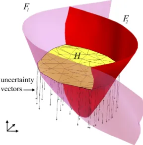
Figure 1: Topology changes induced by geometrical changes. In the reference case, the horizon H is in between faults F1and F2. A simple drift of H along uncertainty vectors may completely change the
configuration: H could possibly occur on either side of F1or F2and not anymore in between the two faults.
Fig. 1. Changements topologiques induits par des perturbations g´eom´etriques. Dans le cas initial, l’horizon H se situe entre les failles F1et F2. Une simple translation de H le long de vecteurs d’incertitude
peut compl`etement changer la configuration : H pourrait ˆetre en contact avec seulement F1ou F2et ne plus
se situer entre les deux failles.
In explicit modeling, geological interfaces are represented as polygonal surfaces. Lecour et al. [16] propose to modify the geometry of a surface by perturbing its nodes along an uncertainty bar defined at each node. The perturbation is correlated along the
surface using the probability field method [17], in order to obtain realistic geometries. In the case of fault perturbation, curvature sign along the sliding direction is preserved to ensure fault compliance.
Other techniques have been developed to perturb the geometry of structural models, keeping the topology fixed [14, 18–20]. For a whole model, each surface is perturbed according to its structural uncertainties and all connections (horizon to horizon, horizon to fault and fault to fault) are stored. Once all geological objects have been perturbed, connections are honored so that the topology is preserved [16]. In practice, this raises a number of challenges to maintain model consistency in the case of large uncertainties, for interferences between surfaces and large mesh distorsions may occur. Moreover, large geometrical uncertainties may require topology changes, for instance horizon to fault connections (Fig. 1).
2.2. Topological perturbation
Topology is all about connections and relations between objects. In a structural model, topological changes may be introduced in different manners:
• Adding or removing geological objects.
• In the case of faults, changing the truncation rule between two faults.
• During geometrical perturbations, a simple drift of an horizon along uncertainty vectors may induce a topological change (especially fault to horizon connections, Fig. 1).
Few methods have been proposed to change the topology of a structural model. A fault modeling tool, referred to as Havana has been proposed in [21, 22]. It is mainly designed for the oil industry and works directly on a corner-point reservoir grid used for flow simulations. This choice allows for directly observing the effects of structural uncertainties on flow simulations. However, resevoir grids have known shortcomings to accurately represent geological structures. Consequently, sub-seismic faults are added by simply modifying the permeability field. Main faults are bilinear planes parallel to the pillars of the reservoir grid or stair-stepped faults.
In our approach, we borrow the idea of fault operator to [21], but use a flexible rep-resentation of faults. This makes it possible to account for large structural uncertainties without making simplifications due to the grid orientation. For accuracy, this method uses an implicit representation of structural interfaces, as in [23–25].
2.3. Implicit modeling: new perspectives for 3D modeling
An implicit surface (e.g. Fig. 3d) is described by an isovalue f of a monotonic volumetric function F (x, y, z) (e.g. Fig. 3a,c)(e.g. the geological time [26], the signed distance to an object [27]):
F (x, y, z)= f (1) A conforming stratigraphic column is then represented as a set of isopotentials of a same scalar field, whereas unconformities and faults are defined by their own scalar
f
bf
a fa+
→
a. b. c.f
af
b A -+ A + - B∩
A+ -∩BA+
B+
B
∩
A-
B
-
A- +
∩
B
→
→
→
→
→
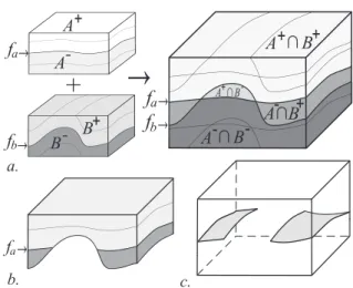
Figure 2: Boolean operations in implicit modeling. a. Left: two surfaces A (FA(x, y, z) = fA) and B
(FB(x, y, z)= fB) and their corresponding half-spaces. Right: boolean sum of the two scalar fields defining
four spatial regions. b. Example of boolean operation: FA(x, y, z) ∩ FB(x, y, z) ≥ fB. c. Example of
truncation corresponding to the operation: FA(x, y, z)= fA∩ FB(x, y, z) ≥ fB(equation 2).
Fig 2. Op´erations bool´eennes en mod´elisation implicite. a. Gauche : deux surfaces A (FA(x, y, z) = fA)
et B (FB(x, y, z) = fB) et leurs demi-espaces. Droite: 4 r´egions spatiales d´efinies par l’intersection des
deux champs scalaires. b. Exemple d’op´eration bool´eenne: FA(x, y, z) ∩ FB(x, y, z) ≥ fB. c. Exemple
d’intersection : FA(x, y, z)= fA∩ FB(x, y, z) ≥ fB(´equation 2).
field. Consequently, horizons can be perturbed independently of faults. Truncations by faults are only honored when an explicit surface is extracted from an isovalue of a scalar field.
Implicit modeling provides a means to easily truncate some surfaces by others using Constructive Solid Geometry (CSG) concepts. For instance, a surface A (FA(x, y, z)=
fA) can be truncated by another implicit surface B (FB(x, y, z) = fB), by making a
boolean intersection between A and either half-spaces of B (Fig. 2). For instance, a truncated surface A|B+is defined by:
FA(x, y, z)= fA|FB(x, y, z) ≥ fB (2)
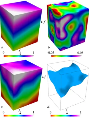
The reference scalar field of an implicit surface (F (x, y, z) = f ) can be perturbed by introducing a correlated random field R(x, y, z) [18]. The new surface is defined by the same isovalue f in the field F (x, y, z)+ R(x, y, z) (Fig. 3).
3. A new method for stochastic simulations of fault networks
The proposed stochastic fault simulation method takes advantage of the implicit surface perturbation and CSG operations between faults. To represent how faults par-tition the domain and interact one with another, we propose using a binary tree.
Figure 3: Geometrical perturbation method in implicit modeling. a. The reference scalar field F (x, y, z) defining the initial implicit surface (isovalue f , planar surface). b. A correlated random field R(x, y, z) generated by Sequential Gaussian Simulation represents the perturbation field. c. The surface is now defined by the isovalue f in the field F (x, y, z)+ R(x, y, z). d. View of the perturbed surface.
Fig 3. M´ethode de perturbation g´eom´etrique en mod´elisation implicite. a. Le champ scalaire de r´ef´erence F (x, y, z) d´efinit la surface initiale (isovaleur f , surface plane). b. Un champ al´eatoire corr´el´e g´en´er´e par une Simulation S´equentielle Gaussienne correspond au champ de perturbation. c. La surface est maintenant d´efinie par l’isovaleur f dans le champ F (x, y, z)+ R(x, y, z). d. Surface perturb´ee.
3.1. Binary trees as descriptors of fault relationships
Indeed, each fault divides the model M in two distinct fault blocks B−and B+[28],
defined by:
• B−= {(x, y, z) ∈ M|F (x, y, z) < f } • B+= {(x, y, z) ∈ M|F (x, y, z) > f }
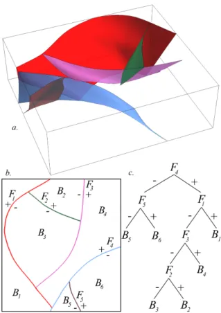
Then, in the binary tree representing a fault network, each node represents a fault and each leave (node without children) represents a fault block (Fig. 4).
Each fault in the tree is potentially a branching fault for its parent faults in the tree. Switching a parent and its child in the tree changes their relationship: the main fault becomes the branching fault and inversely (Fig. 5). A special case may occur when a
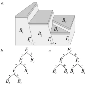
Figure 4: A fault network and its topological representation as a binary tree. a. Fault network in 3D. b. The same model in top view to make the topology more explicit. Each fault Fidivides the model in two blocks
Bi. c. Binary tree representing the fault relationships. The fault F4is the main and oldest fault (root node of
the tree), other faults are branching faults.
Fig. 4. Un r´eseau de failles et sa repr´esentation topologique en arbre binaire. a. R´eseau de failles en 3D. b. Le mˆeme mod`ele vu de dessus afin d’expliciter la topologie. Chaque faille Ficoupe le mod`ele en
deux blocs Bi. c. Arbre binaire repr´esentant les relations entre failles. La faille F4est la faille principale
(racine de l’arbre), les autres failles ´etant des failles secondaires.
fault F cuts a set of older faults Sold = {Fi|i ∈ [1, n]}. In this case, the oldest faults Sold
are on both sides of the cutting fault F in the 3D model, hence they appear in the two branches of F in the tree (Fig. 5c).
When modeling a given fault array, some faults may not be truncated by other faults. Therefore, individual faults can be considered either parent or child in the bi-nary tree, there is no consequence in term of truncation since faults are not in contact. Consequently, a given fault network may be described by several binary trees (Fig. 6). As there is no one-to-one correspondence between a fault network and a binary tree, the latter should be considered as a hierarchy of fault events, the oldest fault being the root of the tree, except for faults offset by more recent faults. Nevertheless, a tree fully defines the topology of the fault network.
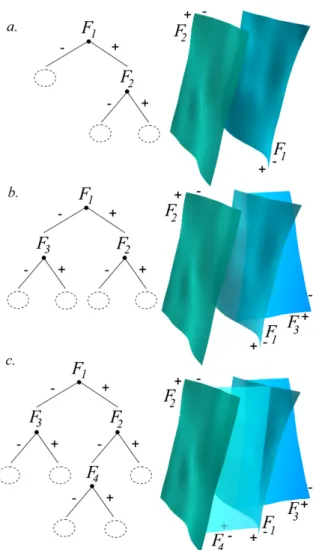
Figure 5: Consequences of filiation relationships in a binary tree from a geological point of view. a. The fault F1is the root, F2is a branching fault. b. Inversion of the relationship. F1is now a branching fault. c.
A fault F2being on both sides of F1means that F2is cut by F1. F2is the child of F1in the tree although it
is the oldest fault.
Fig. 5. Cons´equences des relations de filiation dans un arbre binaire d’un point de vue g´eologique. a. La faille F1est la racine de l’arbre, F2est la faille secondaire. b. Inversion de la relation p`ere-fils. F1est
maintenant la faille secondaire. c. Une faille F2pr´esente des deux cˆot´es de F1signifie que F2est recoup´ee
par F1. F2est la fils de F1dans l’arbre bien qu’elle soit plus ancienne.
3.2. Fault array simulations 3.2.1. Fault network composition
We consider a fault network composed of one or several fault families. Fault fami-lies regroup faults having similar structural parameters (orientation, type). If only a few data about a fault family is available, it can be described by statistical input parameters:
• a relative age • a number of faults
• orientation (dip and strike) distributions • perturbation parameters
Alternatively, fault families may be described by any scalar field (e.g. coming from the interpolation of field, borehole or seismic data) and perturbation parameters defining the associated uncertainties. The key input parameter is the relative age of faults since it determines the order of simulation and thus the place in the binary tree (section 3.2.3).
To simulate a fault array, only one binary tree is needed, containing all the faults of the network. Different fault networks are obtained by generating different binary trees. 3.2.2. Method for simulating a fault
• Add a leaf randomly in the tree (i.e. choose randomly a fault block).
• Define the initial fault surface by a reference field F (x, y, z) from statistical pa-rameters or input scalar field.
• Perturb the initial geometry by simulating a noise R(x, y, z) using a Sequential Gaussian Simulation, set to 0 perturbation at data location (method presented in Fig. 3).
• Define the fault by the field F0(x, y, z)= F (x, y, z) + R(x, y, z).
• Draw an isovalue f from the range of values that occurs in the selected block to define the fault by F0(x, y, z)= f .
For a model M containing n fault blocks Bi|i∈[1,n], let be pithe probability for the
block Bito be selected for containing the new fault, with n
X
i=1
pi= 1. Different strategies
are possible to define pi|i∈[1,n]. For instance, a uniform probability law can be used:
pi|i∈[1,n]=
1
n (3)
Using this strategy, no block is priviledged and fault blocks totally different in volume may be obtained. Another strategy consists in balancing the probability by the volume Viof the block Bi:
pi|i∈[1,n]= Vi n X i=1 Vi (4)
The volume of a block defined by several implicit faults can be calculated using the method presented in [29].
Once a block Bselected has been drawn, an isovalue f corresponding to the fault
(F0(x, y, z)= f ) can be drawn in Bselectedin different manners. As for selecting a block,
each location in the block can be equiprobable. Therefore the isovalue can be drawn from a uniform law whose extremities are the minimum and maximum values of the field F0(x, y, z) in the block Bselected. However, as observed in [21, 22], main
sub-seismic faults tends to repulse each other. A simple way to simulate such a behavior is to draw the isovalue corresponding to the fault from a symetric triangular or truncated Gaussian law so that medium positions in the block are priviledged.
3.2.3. Order of simulation
In the general case, fault families are simulated in chronological order, the oldest one first. Consequently, all the faults belonging to the same family are branching faults for the faults belonging to older families (Fig. 7).
3.2.4. Case of cogenetic faulting
Faults with different structural characteristics (i.e., belonging to different families) may initiate simultaneously at the geological time scale and thus truncate each other. One example of such a situation are conjugate faults, corresponding to steeply opposed-dipping faults. In this case, fault families cannot be simulated one after the other. Instead, let be Scoeval the set of all the faults to be simulated belonging to cogenetic
families. The method is iterative: a fault is drawn in the set Scoevaland added randomly
in the binary tree, until Scoevalis empty. Consequently, faults belonging to a given
fam-ily may be parent or child for the other cogenetic families, hence different truncation rules between families (Fig. 8d).
Figure 6: Non uniqueness of the representation of a fault array in a binary tree. a. 3D diagram representing three faults. The faults F1and F2are not in contact so they can either be parent or child in the binary tree.
b. Representation of the three faults in a binary tree with F1as the parent fault. c. F2is now the root of the
tree without any change about their truncation in the diagram. There may be a consequence of the change deeper, outside the diagram.
Fig. 6. Non unicit´e de la repr´esentation d’un ensemble de failles dans un arbre binaire. a. Dia-gramme 3D repr´esentant 3 failles. Les failles F1et F2ne sont pas en contact. Par cons´equent, elles peuvent
ˆetre p`ere ou fils dans l’arbre binaire. b. Arbre binaire avec F1en tant que faille parente. c. F2est maintenant
la racine de l’arbre mais aucun recoupement n’a chang´e. Il se peut que le recoupement change plus en profondeur, en dehors du diagramme.
3.2.5. Case of cross-cutting faults
A special situation may occur when a fault is offset by other faults (Fig. 5c). Indeed, in this case, the parent fault in the tree is the youngest one. This situation can be obtained by simulating the youngest fault Fyoung(Fyoung(x, y, z)= fyoung) first and then
simulating the shifted fault Fshi f ted in a block (adding it at one leaf as usually). Then,
another leaf. Assuming no rotation of Fyoung’s displacement, Fshi f ted is defined by the
same scalar field but by different isovalues depending on the fault block: • Fshi f ted(x, y, z)= f−|Fyoung(x, y, z) ≤ fyoung
• Fshi f ted(x, y, z)= f+|Fyoung(x, y, z) ≥ fyoung
4. Perspectives and conclusion
We have introduced a new framework for modeling structural uncertainties. In par-ticular, the method goes beyond the perturbation of deterministic 3D structural interpre-tations, but considers the uncertainty about connectivities between structural interfaces (Fig. 8). We expect this method to provide a basis for further advances in subsurface uncertainty management, including:
• Taking into account additional data, e.g. field and seismic data, size distribution, slip information. In the case seismic data is available, the global vertical dis-placement is known for the fault zone. The sum of the simulated disdis-placement for all the faults present laterally in the zone must be equal to the displacement known from seismic data. Some work has also be done to underline the correla-tion between the displacement of a fault and its size [30, 31]. Such correlacorrela-tions could be used either to simulate the displacement or laterally dying and synsedi-mentary faults, depending on the available data.
• How to model particular fault zones? Using our method, realistic fault arrays are obtained but not particular configurations. One may want to simulate, e.g. a fault relay zone, for there are evidence such a structure occurs in the studied area although uncertainties remain. For instance, the probability of a breaching fault to connect two segments of a relay zone must only be defined for the block in between the two segments. It means that some blocks cannot be selected during the simulation, i.e. the binary tree structure is constrained.
• Flower structures between two faults is another challenge since in this case, each fault is both parent and child of the other fault, corresponding to cycles in the tree. To solve this problem, the geometry of a flower structure may be obtained by considering one main fault depending on the sliding direction and an inactive lentil bounded to the sliding surface [32].
The method takes advantage of implicit modeling for both topology description and changes. Each fault is fully described by a monotonic volumetric function F0(x, y, z)
corresponding to the sum of a reference field F (x, y, z), computed from statistical or hard data, and a spatially correlated random field R(x, y, z) corresponding to the asso-ciated uncertainties. We believe this implicit representation provides a convenient and robust way of guaranteeing the model consistency.
A binary tree has been introduced to describe the spatial relationships between faults. The tree should be considered as a descriptor of fault events, a fault being a branching fault for its ascending branch in the tree. During the fault simulation, faults
Figure 7: Steps for generating a fault network. a. Two faults belonging to the same family and the corresponding tree have been simulated. Two faults belonging to another fault family remain to simulate. b. One leaf of the tree is drawn depending on the random function used (e.g. uniform, balanced by block’s volume). Once a block is selected, the algorithm generates a field for the next fault and perturbs it using the method presented in Fig.3. Then, an isovalue is drawn among the range of values present in the selected block. c. The same process is repeated to add another fault.
Fig. 7. Etapes de la g´en´eration d’un r´eseau de failles.´ a. Deux failles appartenant `a la mˆeme famille ainsi que l’arbre binaire correspondant ont d´ej`a ´et´e simul´es. Deux failles appartenant `a une autre famille doivent encore ˆetre ajout´ees. b. Un bloc est tir´e selon une fonction al´eatoire (ex., uniforme, proportionnelle au volume des blocs). Une fois le bloc s´electionn´e, un champ scalaire est simul´e pour la prochaine faille en utilisant la m´ethode pr´esent´ee en Fig.3. Une isovaleur est ensuite tir´ee parmi les valeurs pr´esentes dans le bloc. c. Le mˆeme proc´ed´e est r´ep´et´e afin d’ajouter une faille suppl´ementaire.
are added in the tree according to their relative age in order to obtain a fault network honoring input structural constraints. Fault arrays with different topologies are obtained
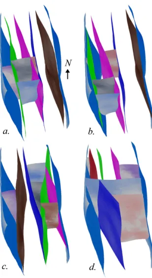
Figure 8: Simulation results illustring different levels of structural uncertainties in a vertical fault zone. a − b: low uncertainty, only the geometry of fault surfaces is uncertain, the connectivity is fixed. c − d: large uncertainty, both the geometry and the connectivity are uncertain. In c, the fault family oriented NS is the main family, the second fault family oriented WS is branching on the first family. In d, even the faulting events are uncertain, fault families are considered as cogenetic families.
Fig. 8. R´esultats de simulation illustrant diff´erents niveaux d’incertitude dans une zone de faille verticale. a − b: faible incertitude, seule la g´eom´etrie des failles est incertaine, la connectivit´e est fixe. c − d incertitude importante, la g´eom´etrie ainsi que la connectivit´e des failles sont incertaines. Pour le cas c, la famille de faille orient´ee Est-Ouest est secondaire par rapport `a la famille de faille orient´ee Nord-Sud. Pour le cas d, l’ordre chronologique des deux ´ev`enements de fracturation est incertain, ce qui revient `a consid´erer les deux familles de faille cog´en´etiques.
Such a multi-realization approach enables to assess the inherent uncertainties to geological data sets. Existing methods are mostly used in the oil industry to reduce economical risks. However, we believe it has a strong potential in other application fields such as potential field interpretation or seismic waveform inversion.
Acknowledgements
This research was performed in the frame of the gOcad research project. The com-panies and universities members of the gOcad consortium are acknowledged for their support, as well as Paradigm Geophysical for also providing the Gocad software and API. This is CRPG contribution 2020.
References
[1] J.-P. Chil`es, P. Delfiner, Geostatistics: Modeling Spatial Uncertainty, Series in Probability and Statistics, John Wiley and Sons, 1999, 696p.
[2] P. Goovaerts, Geostatistics for natural resources evaluation, Applied Geostatis-tics, Oxford University Press, New York, NY, 1997, 483p.
[3] N. Remy, A. Boucher, J. Wu, Applied Geostatistics with SGeMS: A User’s Guide, Cambridge University Press, 2008, 284p.
[4] C. A. Guzofski, J. P. Mueller, J. H. Shaw, P. Muron, D. A. Medwedeff, F. Bilotti, C. Rivero, Insights into the mechanisms of fault-related folding provided by volumetric structural restorations using spatially varying mechanical constraints, AAPG Bulletin 93 (4) (2009) 479–502.
[5] A. Paluszny, S. K. Matthai, M. Hohmeyer, Hybrid finite elementfinite volume dis-cretization of complex geologic structures and a new simulation workflow demon-strated on fractured rocks, Geofluids 7 (2) (2007) 186–208.
[6] J. F. Thompson, B. K. Soni, N. P. Weatherill, Hand Book of Grid Generation, CRC Press, New York, 1999.
[7] R. Frodeman, Geological reasoning: geology as an interpretive and historical science, Geological Society of America Bulletin 107 (8) (1995) 960–968. [8] C. Bond, A. Gibbs, Z. Shipton, S. Jones, What do you think this is? ”conceptual
uncertainty” in geoscience interpretation, GSA Today 17 (11) (2007) 4–10. [9] G. K. Gilbert, The inculcation of scientific method by example, American Journal
of Science 31 (1886) 284–299.
[10] T. C. Chamberlin, The method of multiple working hypotheses, Science 15 (1890) 92–96.
[11] P. Samson, O. Dubrule, N. Euler, Quantifying the impact of structural uncer-tainties on gross-rock volume estimates, in: NPF/SPE European 3D Reservoir Modelling Conference (SPE 35535), 1996, pp. 381–392.
[12] T. Manzocchi, A. E. Heath, B. Palananthakumar, C. Childs, J. J. Walsh, Faults in conventional flow simulation models: a consideration of representational assump-tions and geological uncertainties, Petroleum Geoscience 14 (1) (2008) 91–110. [13] G. Vincent, B. Corre, P. Thore, Managing structural uncertainty in a mature field
for optimal well placement, in: SPE Reservoir Evaluation & Engineering, Vol. 2, 1999, pp. 377–384.
[14] S. Suzuki, G. Caumon, J. Caers, Dynamic data integration for structural model-ing: model screening approach using a distance-based model parameterization, Computational Geosciences 12 (2008) 105–119.
[15] A. Tarantola, Popper, bayes and the inverse problem, Nature Physics 2 (2006) 492–494.
[16] M. Lecour, R. Cognot, I. Duvinage, P. Thore, J.-C. Dulac, Modeling of stochastic faults and fault networks in a structural uncertainty study, Petroleum Geoscience 7 (2001) S31–S42.
[17] R. M. Srivastava, R. Froidevaux, Probability field simulation: A retrospective, in: Geostatistics Banff 2004, Springer, 2004, pp. 55–64.
[18] G. Caumon, A.-L. Tertois, L. Zhang, Elements for stochastic structural perturba-tion of stratigraphic models, in: Proc. Petroleum Geostatistics, EAGE, 2007. [19] T. Charles, J. M. Gu´em´en´e, B. Corre, G. Vincent, O. Dubrule, Experience with the
quantification of subsurface uncertainties, Paper presented at SPE Asia Pacific Oil and Gas Conference and Exhibition, Jakarta, Indonesia, SPE 68703, 17–19 April. [20] P. Thore, A. Shtuka, M. Lecour, T. Ait-Ettajer, R. Cognot, Structural uncertain-ties: determination, management and applications, Geophysics 67 (3) (2002) 840–852.
[21] L. Holden, P. Mostad, B. F. Nielsen, J. Gjerde, C. Townsend, S. Ottesen, Stochas-tic structural modeling, Math. Geol. 35 (8) (2003) 899–914.
[22] K. Hollund, P. Mostad, B. F. Nielsen, L. Holden, J. Gjerde, M. G. Contursi, A. J. McCann, C. Townsend, E. Sverdrup, Havana - a fault modeling tool, in: A. G. Koestler, R. Hunsdale (Eds.), Hydrocarbon Seal Quantification. Norwe-gian Petroleum Society Conference, Stavanger, Norway, Vol. 11 of NPF Special Publication, Elsevier Science, 2002, pp. 157–171.
[23] P. Calcagno, J. Chil`es, G. Courrioux, A. Guillen, Geological modelling from field data and geological knowledge: Part i. modelling method coupling 3d potential-field interpolation and geological rules, Physics of the Earth and Planetary Interi-ors 171 (1-4) (2008) 147 – 157, recent Advances in Computational Geodynamics: Theory, Numerics and Applications.
[24] T. Frank, A.-L. Tertois, J.-L. Mallet, 3d-reconstruction of complex geological interfaces from irregularly distributed and noisy point data, Computers & Geo-sciences 33 (7) (2007) 932 – 943.
[25] A. Guillen, P. Calcagno, G. Courrioux, A. Joly, P. Ledru, Geological modelling from field data and geological knowledge: Part ii. modelling validation using gravity and magnetic data inversion, Physics of the Earth and Planetary Interiors 171 (1-4) (2008) 158 – 169, recent Advances in Computational Geodynamics: Theory, Numerics and Applications.
[26] J.-L. Mallet, Space-time mathematical framework for sedimentary geology, Mathematical geology 36 (1) (2004) 1–32.
[27] D. Ledez, Mod´elisation d’objets naturels par formulation implicite, Ph.D. thesis, INPL, Nancy, France (2003).
[28] A.-L. Tertois, J.-L. Mallet, Distance maps and virtual fault blocks in tetrahedral models, 26thGocad Meeting, Nancy, June (2006).
[29] J.-J. Royer, Conditional integration of a linear function on a tetrahedron, 25th
Gocad Meeting, Nancy, June (2005).
[30] J. J. Walsh, J. Watterson, Analysis of the relationship between displacements and dimensions of faults, Journal of Structural Geology 10 (3) (1988) 239–247. [31] P. A. Gillespie, J. J. Walsh, J. Watterson, Limitations of dimension and
displace-ment data from single faults and the consequences for data analysis and interpre-tation, Journal of Structural Geology 14 (10) (1992) 1157–1172.
[32] J. J. Walsh, J. Watterson, W. R. Bailey, C. Childs, Fault relays, bends and branch-lines, Journal of Structural Geology 21 (8-9) (1999) 1019 – 1026.