A variable streamflow velocity method for global river routing model: model description and preliminary results

(1)

HAL Id: hal-00298918

https://hal.archives-ouvertes.fr/hal-00298918

Submitted on 13 Dec 2007

HAL is a multi-disciplinary open access

archive for the deposit and dissemination of sci-entific research documents, whether they are pub-lished or not. The documents may come from teaching and research institutions in France or abroad, or from public or private research centers.

L’archive ouverte pluridisciplinaire HAL, est destinée au dépôt et à la diffusion de documents scientifiques de niveau recherche, publiés ou non, émanant des établissements d’enseignement et de recherche français ou étrangers, des laboratoires publics ou privés.

A variable streamflow velocity method for global river

routing model: model description and preliminary

results

T. Ngo-Duc, T. Oki, S. Kanae

To cite this version:

T. Ngo-Duc, T. Oki, S. Kanae. A variable streamflow velocity method for global river routing model: model description and preliminary results. Hydrology and Earth System Sciences Discussions, Euro-pean Geosciences Union, 2007, 4 (6), pp.4389-4414. �hal-00298918�

(2)

HESSD

4, 4389–4414, 2007

A variable velocity method for global river routing model

T. Ngo-Duc et al. Title Page Abstract Introduction Conclusions References Tables Figures ◭ ◮ ◭ ◮ Back Close

Full Screen / Esc

Printer-friendly Version Interactive Discussion

EGU Hydrol. Earth Syst. Sci. Discuss., 4, 4389–4414, 2007

www.hydrol-earth-syst-sci-discuss.net/4/4389/2007/ © Author(s) 2007. This work is licensed

under a Creative Commons License.

Hydrology and Earth System Sciences Discussions

Papers published in Hydrology and Earth System Sciences Discussions are under open-access review for the journal Hydrology and Earth System Sciences

A variable streamflow velocity method for

global river routing model: model

description and preliminary results

T. Ngo-Duc, T. Oki, and S. Kanae

Institute of Industrial Science, University of Tokyo, Japan

Received: 13 November 2007 – Accepted: 21 November 2007 – Published: 13 December 2007

(3)

HESSD

4, 4389–4414, 2007

Full Screen / Esc

EGU

Abstract

This paper presents an attempt of simulating daily fluctuations of river discharge at global scale. Total Runoff Integrating Pathways (TRIP) is a global river routing model which can help to isolate the river basins, inter-basin transport of water through river channels, as well as collect and route runoff to the river mouths for all the major rivers.

5

In the previous version of TRIP (TRIP 1.0), a simple approach of constant river flow velocity is used. In general, that approach is sufficient to model mean long-term dis-charges. However, to model short-term fluctuations, more sophisticated approach is required. In this study, we implement a variable streamflow velocity method to TRIP (TRIP 2.0) and validate the new approach over the world’s 20 major rivers. Two

nu-10

merical experiments, one with the TRIP 1.0 and another with TRIP 2.0 are performed. Input runoff is taken from the multi-model product provided by the second Global Soil Wetness Project. For the rivers which have clear daily fluctuations of river discharge, TRIP 2.0 shows advantages over TRIP 1.0, suggesting that TRIP 2.0 can be used to model flood events.

15

1 Introduction

Understanding the movement of water over the earth’s surface has long been a fas-cinating research target. Many hydrologic studies have been done to determine the quantity of flow along rivers at various points in time and space. Most of these studies have focused on small watersheds. Recently with the technology development and the

20

concerns about global climate change, the climate modeling community has focused attention on the need for routing models to track the flow of water from continents to oceans at global scale.

Several advantages of routing models can be listed here. First, routing runoff pro-vides a basis for comparing and validating estimates of streamflow with observed

hy-25

(4)

HESSD

4, 4389–4414, 2007

Full Screen / Esc

EGU observable, river discharge is an appropriate measure to assess model qualities.

Sec-ond, the simulated fresh water flux into the oceans alters their salinity and may affect the thermohaline circulation (e.g. Wang et al., 1999; Wijffels et al., 1992). Third, esti-mates of river discharge from climate change simulations can also be used to assess the impact of climate change on water resources and the hydrology of the major river

5

basins (e.g. Arora and Boer, 2001; Milly et al., 2005; Oki and Kanae, 2006). Ap-proaches for routing water through large-scale systems are thus evolving in response to the modeling needs.

In state-of-the-art global routing models, most of the approaches either assume a constant velocity (e.g. Miller et al., 1994; Coe, 1998; Oki et al., 1998) or use simple

10

formulae that use time-independent flow velocities parameterized as a function of the topographic gradient (Miller et al., 1994; Hagemann and D ¨umennil, 1996; Ducharne et al., 2003). In general, these approaches are sufficient to model discharges in monthly or longer time scales. However, to model in shorter temporal scales, more sophis-ticated approach is required. Arora and Boer (1999) and more recently, Schulze et

15

al. (2005) use the Manning’s equation to determine time-evolving flow velocities as a function of discharge, river cross-section and channel slope:

v=n−1

×R2/3×s1/2 (1)

wherev is the flow velocity [m/s], n is the Manning roughness coefficient [−], R is the

hydraulic radius [m], and s is the channel slope [m/m]. In their studies, the Manning

20

roughness coefficient n is supposed to be constant globally (Arora and Boer, 1999) or determined by tuning (Schulze et al., 2005). Since values ofn vary between 0.015 and

0.07 in natural streams for flows less than bankfull discharge and reach up to 0.25 for overbank flow (Fread, 1993), the assumption of a global constant roughness coefficient or the tuning method would contain limitations.

25

Dingman and Sharma (1997) developed the following relation from objective statisti-cal analysis of over 500 in-bank flows:

(5)

HESSD

4, 4389–4414, 2007

Full Screen / Esc

EGU whereQ [m3/s] andA [m2] are river discharge and cross-sectional area respectively.

Note that:

Q=A×v (3)

We can induce that Eq. (2) is another representation of the Manning equation (Eq. 1) with the roughness coefficient calculated by:

5

n= 1

1.564×A

−0.173

×R0.267×s0.5+0.0543× log10s (4) Thus, Eq. (2) proposed by Dingman and Sharma has potential to overcome the limi-tations of constant roughness coefficient assumption or a tuning procedure for global routing models.

Total Runoff Integrating Pathways (TRIP) is a global river routing model which can

10

help to isolate the river basins, inter-basin tranport of water through river channels, as well as collect and route runoff to the river mouths for all the major rivers (Oki and Sud, 1998). In the previous version of TRIP (hereafter TRIP 1.0), the simple approach of constant river flow velocity was used. In this paper, we implement the Dingman and Sharma equation to TRIP (hereafter TRIP 2.0) and perform the validation of the new

15

approach over the Mekong and some other world’s largest rivers.

2 Methodology

In TRIP 2.0, we define two water reservoirs: groundwater reservoir and surface water reservoir. Groundwater is represented by a simple linear reservoir (e.g. Maidment, 1993):

20

d S_g

(6)

HESSD

4, 4389–4414, 2007

Full Screen / Esc

Printer-friendly Version Interactive Discussion EGU whereS_g [m3],DLSMg[m 3 /s], andDOUTg[m 3

/s] are groundwater storage, input subsur-face runoff (obtained from the output of Land Sursubsur-face Model (LSM)), and the outflow from the groundwater reservoir, respectively. The outflow is parameterized as:

DOUTg=

1

T_g×Sg (6)

whereT_g is a groundwater delay parameter expressed in days.

5

From Eq. (5) and Eq. (6), we obtain the solution forSg:

S_g(t+dt)=e−d t/Tg_×S

g(t)+(1−e−d t/Tg)×Tg×DLSMg(t+dt) (7)

IfTg=0, we define Sg=0, DOUTg=DLSMg, i.e. TRIP 2.0 will route the total runoff and not separate anymore surface runoff and subsurface runoff.

The water balance within a grid cell for the surface water reservoir storage,S_s [m3],

10 is given by: d S_s d t =Dup+DOUTg+DLSMs−Q (8) whereDup [m 3 /s] andDLSMs[m 3

/s] are total inflow from upstream grid boxes and sur-face runoff calculated by LSM, respectively.

The volume of water in the river channel is:

15

S_s=A×l ×rM (9)

wherel is the straight length of the river channel within the grid box calculated

geomet-rically andrM is the meandering ratio (Oki and Sud, 1998) adjusting the river length to

be realistic. In this study, we setr_M=1.4 globally.

Substituting Eq. (3), Eq. (9) into the continuity equation Eq. (8) yields:

20 d S_s d t =Dup+DOUTg+DLSMs− v l ×rM ×Ss (10)

(7)

HESSD

4, 4389–4414, 2007

Full Screen / Esc

EGU One should note thatv depends itself on Ss. To solve Eq. (10), we assume that v is

constant during each time step.

We obtain thus the solution of Eq. (10)

S_s(t+dt)=e−d t×_{l ×rM}v(t) ×Ss(t)+(1−e−d t× v(t) l ×rM_)×l ×rM v(t) ×(Dup(t+dt)+DOUTg(t+dt)+DLSMs(t+dt)) (11) 5

wherev(t) is calculated in the time step t as followings:

From Eq. (2), Eq. (3),v can be described as:

v=1.564×A0.173×R0.400×s−0.0543× log10s (12)

Assuming the river channel is shaped as a rectangle of widthW [m] and depth h [m],

thus we have:

10

R= h×W

2×h+W (13)

W is obtained using a geomorphological relationship with annual mean discharge Qm

[m3s−1_{] proposed by Arora and Boer (1999):}

W = max(10, (6.0+10−4_×Q

m.mouth)×Q0m.5) (14)

whereQm.mouth[m

3

s−1_{] is the annual mean discharge at the river mouth. Sensitivity of}

15

flow velocity to river width has shown that an error of 100% in the prescribed river width results in a corresponding error of about 25% in flow velocity (Arora and Boer, 1999).

Qmis initially calculated from TRIP 1.0, the constant velocity version of TRIP.

Eq. (12) thus becomes:

v=1.564×s−0.0543× log10s_× S 0.573 s (l ×rM)0.573×(_{l ×r}2×Ss M×W+W ) 0.400 (15) 20

(8)

HESSD

4, 4389–4414, 2007

Full Screen / Esc

EGU

3 Experiments design

3.1 Input runoff forcing

The second Global Soil Wetness Project (GSWP2) (International GEWEX Project Of-fice, 2002; Dirmeyer et al., 2006) is an ongoing environmental modeling research ac-tivity aiming at producing global estimates of soil moisture, temperature, snow water

5

equivalent, and surface fluxes by integrating one-way uncoupled LSMs using externally specified surface forcing and standardized soil vegetation distributions. In May 2005, 15 institutes from five nations have submitted their baseline run, and model ensem-ble mean (or simple arithmetic average of outputs among models) of surface fluxes and state variable have been produced using 13 models (Dirmeyer et al., 2006). Gao

10

and Dirmeyer (2006) compared the products (GSWP2-Multi Model Analysis, hereafter GSWP2-MMA) with in-situ soil moisture observation from the Global Soil Moisture Data Bank (Robock et al., 2002) and found that GSWP2-MMA is better than the best indi-vidual model at any location in the representation of both soil wetness and its anomaly. The GSWP2-MMA data, as well as the data submitted by the participating

model-15

ing groups conform to the Assistance for Land-surface Modelling Activities convention (ALMA) (Polcher et al., 2000). The data has 1 degree by 1 degree (longitude-latitude) spatial resolution, and daily temporal resolution spanning the years 1986–1995.

All models (and GSWP2-MMA) provide two runoff variables: surface runoff and sub-surface runoff. However, the partition of runoff into sub-surface and subsub-surface varies

sig-20

nificantly between models. Thus in this study, TRIP 2.0 is used to route total runoff from GSWP2-MMA on a digital river network map with a spatial resolution of 1 degree longitude by 1 degree latitude.

3.2 Numerical experiments

Two numerical experiments are performed. The first one, called T1 is obtained with the

25

(9)

HESSD

4, 4389–4414, 2007

Full Screen / Esc

EGU velocity is assumed constant and uniform at 0.5 m s−1 _{(e.g. Decharme and Douville,}

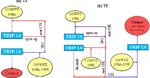
2007; Oki and Sud., 1998). The second one, called T2 is obtained with TRIP 2.0 which used the new variable velocity approach. Both simulations use the GSWP2-MMA runoff of 1986 for spin-up (Fig. 1). Water storage in the river channels is initialized with zero value. The spin-up procedure is finished when the difference of water storage between

5

the 1st January 1987 and the 1st January 1986 is less than 5% for more than 95% of the whole grid cells. For T2, we use the TRIP 1.0 version in the beginning to initialize the value of annual mean discharge required by Eq. (14).

River slopes, which is not required in T1, plays an important role in T2 (see Eq. 15). s is calculated from the 1 degree digital elevation and the drainage flow direction maps

10

created by Oki and Sud (1998). However as consequence of the corrections which were applied to create a more realistic flow direction map, there are many grid points having negative slope values due to the fact that the downstream points have higher elevation. We thus generally set a minimum river slope value of 10−6_{m m}−1 _{(i.e. 0.1 m} per 100 km) to avoid those irregular points.

15

In both T1 and T2, we set the meandering value, rM to 1.4 globally. For simplicity

reason, and for avoiding the inconsistency among the GSWP2 models in the partition of total runoff into surface and subsurface components, the groundwater mode is switched off (i.e. Tg=0). Time step of the simulation is set to 6-hourly.

The sensitivity of river discharge simulated by TRIP to all the above

parame-20

ters/model settings will be discussed in our further paper.

4 Results

4.1 Over the mekong

The Mekong River is the 12th longest river in the world, runs 4800 km from its head-waters on the Tibetan Plateau through Yunnan Province of China, Burma, Thailand,

25

(10)

HESSD

4, 4389–4414, 2007

Full Screen / Esc

EGU middle reaches running through China, while the lower reaches outside China are

known as the Mekong. From 1986 onwards, China began to build eight hydroelectric dams and two reservoirs on the waterway in Yunnan, where the Lancang traverses more than 1000 km, to lift the backward western region out of poverty. The first dam at Manwan, was finished in June 1995. While the GSWP2-period is for 1986–1995, our

5

result would not be affected by the dam’s operations.

In this section, we will access the quality of T1 and T2 over the Mekong by comparing the simulated and observed river discharges.

The river discharge observations used in this study are the daily data obtained from the Global Runoff Data Center (GRDC). In the GRDC data, there are 12 stations over

10

the Mekong. However, only 6 of them overlap the GSWP2 simulation period (1986– 1995). The 3 stations Nong Khai, Near Vieanntiane and Chiang Khan are closely located (or coincide) on the 1 degree flow direction map created by Oki et al. (1998). We use thus the most downstream station, NongKhai, among those 3 stations. Then, the stations over the Mekong which are used to validate our simulation results are:

15

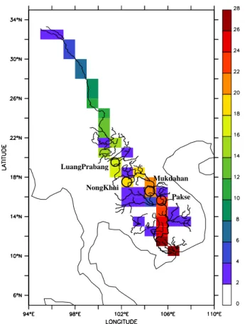
Luang Prabang, NongKhai, Mukdahan, Pakse (see Table 1 and Fig. 2).

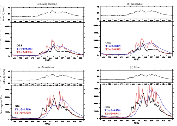
Figure 3 represents a time-series comparison of river discharge for T1, T2 and the observations over the year 1990. The average upstream velocity variations simulated by T2 are also displayed in Fig. 3. In the high flow season, T2 shows that flow velocity can reach to 3 m s−1_{while this value is only about 1 m s}−1 _{in the low flow season.}

Vari-20

able streamflow velocity allows a quick response of river discharge to a high precipita-tion event in the upstream region. T2 is thus able to capture the short term fluctuaprecipita-tions (in this study is daily fluctuations) of river discharge over the Mekong.

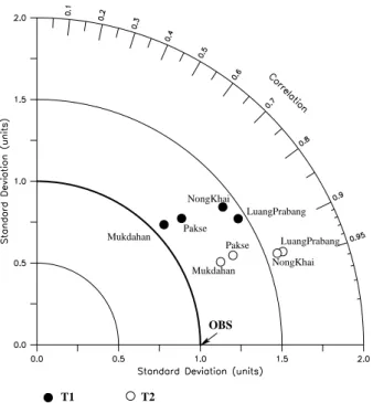
Figure 4 displays a Taylor diagram which shows errors of simulated river discharges for T1 (black filled circles) and T2 (white filled circles). A Taylor diagram (Taylor, 2001)

25

provides the ratio of standard deviation as a radial distance and the correlation with observations as an angle in the polar plot. Each circle corresponds to the quality of simulated discharge at a predefined station. The observed discharge is represented by a point on the horizontal axis (zero correlation error) at unit distance from the origin

(11)

HESSD

4, 4389–4414, 2007

Full Screen / Esc

EGU (no error in standard deviation). In this representation the linear distance between

each simulation result and observed discharge is proportional to the root mean square error (RMSE). Only the overlap period between simulations and observations is used to compute statistics.

For the 4 stations Luang Prabang, Nong Khai, Mukdahan, Pakse, a clear

improve-5

ment of T2 compared to T1 is shown. T2 has smaller RMSE comparing to T1. Partic-ularly the correlations with the observations are well improved, from an average value of 0.78 for T1 to an average value of more than 0.93 for T2.

4.2 Over the world’s largest rivers

The objective of this section is to compare T2 with T1 for other rivers of the world. From

10

the GRDC daily discharge data, 20 stations in 20 major rivers (see Table 2 and Fig. 5) were selected and compared with the simulated discharges. The stations were chosen according to the following criteria:

– Stations which have upstream drainage area greater than 300 000 km2.

– Stations with a minimum observed period of 4 y which overlaps the GRDC 1986–

15

1995 period.

– The most downstream station (i.e. maximum upstream drainage area) among the

available ones on a river which fit the 2 above conditions.

Table 2 represents the stations used for comparing T1 and T2. The correlation (r2) and normal standard deviation (std) between simulated and observed discharges are

20

also displayed in Table 2. Over the period used for comparing, T2 is not statistically better than T1 for most of studying rivers. For some rivers (e.g. the Amazon, Ob, Kolyma), bothr2 and std of T2 are worse than those of T1. For some others (e.g. the Mississippi, Amur, Indigirka), std of T2 is better butr2is worse or vice-versa. For the Brahmaputra and the Mekong, T2 discharge is statistically better than T1.

(12)

HESSD

4, 4389–4414, 2007

Full Screen / Esc

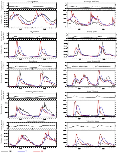
EGU Figure 6 shows daily time-series discharges of T1 and T2 compared to the

obser-vations at the 20 studying stations, over the two year 1987–1988. Over the stations where sub-monthly fluctuations are observed (e.g. the Mississippi, Danube, Brahma-putra, Mekong), T2 shows advantages over T1. Changing river velocity in T2 allows river discharge to vary quickly, which in consequence make T2 be able to represent

5

the sub-monthly observed discharge fluctuations. Over some stations where there are no clear short term fluctuations of river discharge, T2 seems to over-estimate those fluctuations (e.g. over the Amazon, the Orinoco). For the Niger and the Chari in Africa and some other rivers such as the Columbia, the simulated discharges are practically un-correlated with the observations. The reason can be attributed to the GSWP2

pre-10

cipitation quality over those basins and the fact that TRIP does not represent the natural dissipation of water from river channels to surrounding land, water used by the cities, irrigation and dam construction (Ngo-Duc et al., 2005; Hanasaki et al., 2006).

5 Discussion

One can notice that the simulated discharge however is still significantly different from

15

the observations. Understanding the reasons for which such differences occur is im-portant for further study and further development of the routing model. We divide the sources of errors into two main categories, errors originate from the input runoff forcing data and errors originate from the river routing models itself.

The first one is the error due to the input runoff forcing data. In this study, we use

20

the multi-model runoff product from GSWP2. Each LSM participated to GSWP2 has its own approach for calculating runoff. Therefore the runoff can be quite different from one model to another. Gao and Dirmeyer (2006) has compared the GSWP2-MMA products with in-situ soil moisture observation from the Global Soil Moisture Data Bank (Robock et al., 2002) and found that GSWP2-MMA is better than the best individual

25

model at any location in the representation of both soil wetness and its anomaly. For runoff, no such study has been done yet.

(13)

HESSD

4, 4389–4414, 2007

Full Screen / Esc

EGU Runoff quality depends also on the input precipitation of the LSMs (Oki et al., 1999;

Ngo-Duc et al., 2005). Nevertheless, the accuracy and reliability of the 10-y GSWP2 atmospheric forcing remain questionable. Decharme and Douville (2006) showed that the baseline GSWP2 precipitation forcing is generally overestimated over the mid and high latitudes, which implies systematic errors in the simulated discharges.

5

The second source of errors origins from the global river routing model. TRIP con-tains several parameterizations and several assumptions as well as it neglects certain river processes. In the numerical experiments used in this study, TRIP doesn’t take into account the groundwater reservoirs. The current version of TRIP also does not rep-resent the natural dissipation of water from river channels to surrounding land, water

10

used by the cities, irrigation and dam construction.

In T2, drainage flow direction map is used together with the elevation map. Oki and Sud (1998) have created the 1 degree flow direction map from the 1 degree digital elevation map and have applied several corrections (including manual correction in comparison with river pathways available in the atlases). They therefore obtained a

15

more realistic map of flow direction. However as consequence of the corrections, there are many grids points on the 1 degree map having negative slope value due to the fact that the downstream points have higher elevation (see Fig. 7). This suggests a further study of adjusting the digital elevation map to fit the new flow direction map or further simulations using some new global hydrological datasets recently available

20

(e.g. HydroSHEDS by Lehner et al., 2006). In T2, at those irregular points, we use a minimum slope of 10−6_{m m}−1_{instead of the negative values.}

Other reasons of errors which come from TRIP can also be listed here: (a) Eq. (2) and Eq. (14) using in this study are empirical equations obtained for certain rivers and may not be appropriate for everywhere; (b) the meandering value of river is set to 1.4

25

globally, although it is 1.3 for rivers with areas larger than 500 000 km2 (Oki and Sud, 1998); (c) the assumption of constant velocity during each time step in order to solve Eq. (10) may also be too rude.

(14)

HESSD

4, 4389–4414, 2007

Full Screen / Esc

EGU empirical equation, meandering coefficient, etc.) would deserve another careful study

in the near future.

6 Conclusions

This study was aimed at constructing a new version of the global river routing model TRIP, based on a variable streamflow velocity approach, in order to simulate shorter

5

time scale fluctuations of river discharge globally. We have used the Dingman and Sharma (1997) equation to represent the relation between river discharge and river geomorphology. Two numerical experiments, T1 obtained with the previous model version TRIP 1.0 and T2 obtained with TRIP 2.0 have been performed. The river discharges simulated T1 and T2 were used to compare with the daily observations

10

from GRDC for the world’s 20 large rivers.

It was shown that, T2 has clear advantages over T1 in representing the short-term fluctuations of river discharges over certain rivers such as the Mekong, the Brahma-putra, the Mississippi, and the Danube. For the rivers where short-term fluctuations of discharge are not clear, T2 is not better than T1. The differences between simulations

15

by TRIP and GRDC observations have been attributed to several sources of errors: errors from the input forcing data and errors from the models itself. A sensitivity study which helps to quantify how much river discharge depends on those factors would be done in the near future.

TRIP 2.0 is a very first step which allows river routing model to represent short-term

20

fluctuations of river discharge at global scale. On the technical side, input and output of TRIP 2.0 are in netCDF format. TRIP 2.0 can be configured to run with different resolutions and can also be extracted to run for only one region of interest in order to economize computer time consuming. More technical information about TRIP 2.0 can be found at:http://hydro.iis.u-tokyo.ac.jp/TRIP2.

25

Acknowledgements. The authors wish to thank N. Hanasaki and P. Yeh for helpful

(15)

HESSD

4, 4389–4414, 2007

Full Screen / Esc

EGU

Science (JSPS) is also greatly acknowledged.

References

Arora, V. K. and Boer, G. J.: Effects of simulated climate change on the hydrology of major river basins, J. Geophy. Res., 106(D4), 3335–3348, 2001.

Arora, V. K. and Boer, G. J.: A variable velocity flow routing algorithm for GCMs, J. Geophy.

5

Res., 104 (D24), 30 965–30 979, 1999.

Coe, M.: A linked global model of terrestrial hydrologic processes: Simulation of modern rivers, lakes and wetlands, J. Geophys. Res., 103, 8885–8899, 1998.

Dingman S. L. and Sharma K. P.: Statistical development and validation of discharge equations for natural channels, J. Hydrol., 1(199),13–35, 1997.

10

Dirmeyer, P. A., Gao, X., Zhao, M., Guo, Z., Oki, T., and Hanasaki, N.: The Second Global Soil Wetness Project (GSWP-2), Multi-model analysis and implications for our perception of the land surface, B. Am. Meteorol. Soc., 87(10),1381–1397, 2006.

Decharme, B. and Douville, H.: Uncertainties in the GSWP-2 precipitation forcing and their impacts on regional and global hydrological simulations, Clim. Dyn., 27, 695–713,

15

doi:10.1007/s00382-006-0160-6, 2006.

Ducharne, A., Golaz, C., Leblois, E., Laval, K., Polcher, J., Ledoux, E., and de Marsily, G.: Development of a high resolution runoff routing model: calibration and application to assess runoff from the LMD GCM, J. Hydrol., 280, 207–228, 2003.

Fread, D. L.: Flow Routing, in Handbook of Hydrology, edited by Maidment, D. R., McGraw-Hill,

20

New York, pp. 10.1–10.36, 1993.

Gao, X. and Dirmeyer, P. A.: Multi-model analysis, validation, and transferability study for global soil wetness products, J. Hydrometeorol., 7(6), 1218–1236, 2006.

Hagemann, S. and D ¨umenil, L.: A parameterization of lateral water flow for the global scale, Clim. Dyn., 14, 17–41, 1998.

25

Hanasaki, N., Kanae, S., and Oki, T.: A reservoir operation scheme for global river routing models, J. Hydrol., 327, 22–41, 2006.

Lehner, B., Verdin, K., and Jarvis, A.: HydroSHEDS Technical Documentation. World Wildlife Fund US, Washington, DC, available athttp://hydrosheds.cr.usgs.gov, 2006.

(16)

HESSD

4, 4389–4414, 2007

Full Screen / Esc

EGU

International GEWEX Project Office: GSWP-2: The Second Global Soil Wetness Project Sci-ence and Implementation Plan, IGPO Publication Series No. 37, 65 pp., 2002.

Maidment, D. R.: Handbook of Hydrology, McGraw-Hill,ISBN 0070397325/9780070397323, 1424 pp., 1993.

Miller, J. R., Russell, G. L. and Caliri, G.: Continental-scale river flow in climate models, J.

5

Clim., 7, 914–928, 1994.

Milly, P. C. D., Dunne, K. A., and Vecchia, A. V.: Global pattern of trends in streamflow and water availability in a changing climate, Nature, 438(7066), 347–350, 2005.

New, M., Hulme, M., and Jones, P.: Representing twentieth-century space-time climate variabil-ity. Part II: Development of a 1901–1990 mean monthly grids of terrestrial surface climate, J.

10

Clim., 13, 2217–2238, 2000.

Ngo-Duc, T., Polcher, J., and Laval, K.: A 53-year forcing data set for land surface models, J. Geophys. Res., 110, D06116, doi:10.1029/2004JD005434, 2005.

Oki, T. and Sud, Y. C.: Design of Total Runoff Integrating Pathways (TRIP) – A global river channel network. Earth Interactions 2., available athttp://EarthInteractions.org, 1998.

15

Oki, T., Nishimura, T., and Dirmeyer, P.: Assessment of annual runoff from land surface models using total runoff integrating pathways (TRIP),J. Meteorol. Soc. Jpn., 77, 235–255, 1999. Oki, T. and Kanae, S.: Global Hydrologic Cycle and World Water Resources, Science, 313,

5790, 1068–1072, doi:10.1126/science.1128845, 2006.

Polcher, J., Cox, P., Dirmeyer, P., Dolman, H., Gupta, H., Henderson-Sellers, A., Houser, P.,

20

Koster, R., Oki, T., Pitman, A., and Viterbo, P.: GLASS – Global Land-Atmosphere System Study, GEWEX News, 10(2), 3–5, 2000.

Robock, A., Vinnikov, K. Y., Srinivasan, G., Entin, J. K., Hollinger, S. E., Speranskaya, N. A., Liu, S., and Namkhai, A.: The Global Soil Moisture Data Bank, Bull. Am. Meteorol. Soc., 81, 1281–1299, 2000.

25

Schulze, K., Hunger, M., and D ¨oll, P.: Simulating river flow velocity on global scale, Adv. Geosci., 5, 133–136, 2005,

http://www.adv-geosci.net/5/133/2005/.

Taylor, K. E.: Summarizing multiple aspects of model performance in a single diagram, J. Geophys. Res., 106, 7183–7192, 2001.

30

Wang, X., Stone, P. H., and Marotzke, J.: Global thermohaline circulation, part I, Sensitivity to atmospheric moisture transport, J. Clim., 12, 71–82, 1999.

(17)

HESSD

4, 4389–4414, 2007

Full Screen / Esc

EGU

(18)

HESSD

4, 4389–4414, 2007

Full Screen / Esc

EGU Table 1. GRDC stations over the Mekong, which have observations overlapping the period

of GSWP2 simulations. The station ID defined by GRDC, the name, the localizations (coun-try, longitude, Lon, and latitude, Lat), the drainage area (given by GRDC) and the discharge observation period at each station are given.

GRDC-No Station Country Lat (◦_N) _{Lon (}◦_E) _{Area (km}2₎ _Period 2469050 Luang Prabang Laos 19.5 101.5 268 000 86–93 2969090 Nong Khai Thailand 17.5 102.5 302 000 86–93 2969100 Mukdahan Thailand 16.5 104.5 391 000 86–93 2469260 Pakse Laos 15.5 105.5 545 000 86–93

(19)

HESSD

4, 4389–4414, 2007

Full Screen / Esc

EGU Table 2. The world’s 20 rivers which have daily discharge observations during the

GSWP2-period (1986–1995). The approximate river length, the name, the station ID defined by GRDC, the drainage area (given by GRDC and by the TRIP river network), the localizations (longitude, Lon, and latitude, Lat) and the discharge observation period at each basin downstream station are given. Correlation (r2) and normal standard deviation (std) between the simulations and the observations are also displayed on the Table.

River Station GRDC-ID Lon Lat Drainage area Period r2

−T1 r2−T2 std−T1 std−T2 (◦_N) ₍◦_E) _(km2 ) 1 Amazon Obidos 3629000 −55.5 −2.5 4 640 300 86–95 0.91 0.63 1.20 1.33 2 Mississippi Vicksburg 4127800 −91.5 32.5 2 964 255 86–95 0.81 0.88 1.69 2.08 3 Ob Salekhard 2912600 66.5 66.5 2 949 998 86–95 0.85 0.11 2.38 3.13 4 Yenisei Igarka 2909150 86.5 67.5 2 440 000 86–95 0.78 0.49 0.84 0.87 5 Lena Kusur 2903420 127.5 70.5 2 430 000 86–94 0.74 0.56 0.57 0.69 6 Amur Komsomolsk 2906900 137.5 50.5 1 730 000 86–90 0.73 0.54 0.77 0.92

7 Mackenzie Arctic red river 4208025 −133.5 67.5 1 660 000 86–95 0.87 0.57 0.79 0.87 8 Volga Volgograd Power Plant 6977100 44.5 48.5 1 360 000 86–95 0.66 0.60 3.11 3.91

9 Orinoco Puente Angostura 3206720 −63.5 8. 5 836 000 86–89 0.92 0.79 0.94 1.00

10 Yukon Pilot station 4103200 −162.5 61.5 831 390 86–95 0.85 0.60 2.28 2.90

11 Danube Ceatal Izmail 6742900 28.5 45.5 807 000 86–89 0.73 0.68 2.34 2.64

12 Niger Niamey 1234150 2.5 13.5 700 000 86–95 0.75 0.46 8.41 10.38

13 Brahmaputra Bahadurabad 2651100 89.5 25.5 636 130 86–91 0.82 0.88 0.69 0.78

14 Columbia The Dalles, OR 4115200 −121.5 45.5 613 830 86–95 0.68 1.76 7.15 8.25

15 Chari Ndjamena 1537100 15.5 12.5 600 000 86–90 0.93 0.67 0.19 0.22

16 Mekong Pakse 2469260 105.8 15.12 545 000 86–93 0.75 1.18 0.91 1.32

17 Kolyma Kolymskaya 2998510 158.5 68.5 526 000 86–95 0.80 1.33 0.71 1.62

18 Severnaya Dvina UST-Pinega 6970250 41.5 64.5 348 000 86–95 0.88 0.54 1.85 2.12

19 Pechora Oksino 6970700 52.5 67.5 312 000 86–95 0.86 0.54 1.23 1.41

(20)

HESSD

4, 4389–4414, 2007

Full Screen / Esc

EGU

5 $ * # ) K + # ) #&) K & K + # 0)

(21)

HESSD

4, 4389–4414, 2007

Full Screen / Esc

Printer-friendly Version Interactive Discussion EGU Pakse Mukdahan LuangPrabang NongKhai

Fig. 2. 1 degree Mekong river sequence map designed by Oki et al. (1998). River information

from the World Data Bank II (WDBII) developed by the U.S. Central Intelligence Agency is superimposed. The discharge stations using in this study are located by the circulars on the 1 degree resolution map.

(22)

HESSD

4, 4389–4414, 2007

Full Screen / Esc

Printer-friendly Version Interactive Discussion EGU Discharge (m3/s) velocity (m/s) Average upstream

(a) Luang Prabang

OBS T1 (r2=0.858) T2 (r2=0.956) (b) NongKhai OBS T1 (r2=0.809) T2 (r2=0.942) (d) Pakse OBS T1 (r2=0.820) T2 (r2=0.941) (c) Mukdahan Discharge (m3/s) velocity (m/s) Average upstream OBS T2 (r2=0.935) T1 (r2=0.789) 5 ? + $ * & #& ) 0 # ) * $

Fig. 3. River discharges simulated by T1 (blue curve), T2 (red curve) compared to the

(23)

HESSD

4, 4389–4414, 2007

Full Screen / Esc

Printer-friendly Version Interactive Discussion EGU LuangPrabang Pakse LuangPrabang NongKhai Mukdahan NongKhai Pakse Mukdahan OBS T1 T2

Fig. 4. Taylor diagram illustrating the statistics of simulated river discharge compared with daily

observations at (a) Luang Prabang station, (b) Nong Khai station, (c) Mukdahan satation, (d) Pakse station.

(24)

HESSD

4, 4389–4414, 2007

Full Screen / Esc

EGU Fig. 5. Upstream of the 20 stations used in this study. Number corresponds to the number of

(25)

HESSD

4, 4389–4414, 2007

Full Screen / Esc

EGU

Amazon, Obidos

Average upstream velocity (m/s)

Discharge (m3/s) Ob, Salekhard Discharge (m3/s) Average upstream velocity (m/s) Yenisey, Igarka Lena, Kusur Average upstream Discharge (m3/s) velocity (m/s) Amur, Komsomolsk Volga, Volgograd Mississippi, Vicksburg

Yukon, Pilot station Orinoco, Puente Angostura

Average upstream

velocity (m/s)

Discharge (m3/s)

Mackenzie, Arctic Red river

Discharge (m3/s) velocity (m/s) Average upstream T2 T1 OBS

Fig. 6a. Daily discharges of T1 and T2 compared to the observations at the 20 studying

(26)

HESSD

4, 4389–4414, 2007

Full Screen / Esc

EGU

Danube, Ceatal Izmail

velocity (m/s)

Average upstream

Discharge (m3/s)

Niger, Niamey

Columbia, The Dalles OR

Mekong, Pakse

Severnaya Dvina, UST−Pinega

Indigirka, Vorontsovo Pechora, Oksino Average upstream velocity (m/s) Discharge (m3/s) Kolyma, Kolymskaya Discharge (m3/s) Average upstream velocity (m/s) Chari, Ndjamena Discharge (m3/s) Average upstream velocity (m/s) Brahmaputra, Bahadurabad Discharge (m3/s) velocity (m/s) Average upstream OBS T1 T2 Fig. 6b. Continued.

(27)

HESSD

4, 4389–4414, 2007

Full Screen / Esc

EGU Fig. 7. Grid points on the 1 degree global map where the river slope is less than zero (i.e. the

downstream point has higher elevation). In T2, the river slope of those points will be set to the minimum river slope value (which is positive).