HAL Id: hal-02625493
https://hal.archives-ouvertes.fr/hal-02625493
Submitted on 26 May 2020
HAL is a multi-disciplinary open access
archive for the deposit and dissemination of
sci-entific research documents, whether they are
pub-lished or not. The documents may come from
teaching and research institutions in France or
L’archive ouverte pluridisciplinaire HAL, est
destinée au dépôt et à la diffusion de documents
scientifiques de niveau recherche, publiés ou non,
émanant des établissements d’enseignement et de
recherche français ou étrangers, des laboratoires
The ıQuad sensor: a new Fourier-based wave front
sensor derived from the 4 quadrants coronagraph
Olivier Fauvarque, Victoria Hutterer, Pierre Janin-Potiron, Julien Duboisset,
Carlos Correia, Benoit Neichel, Jean-Francois Sauvage, Thierry Fusco, Iuliia
Shatokhina, Ronny Ramlau, et al.
To cite this version:
Olivier Fauvarque, Victoria Hutterer, Pierre Janin-Potiron, Julien Duboisset, Carlos Correia, et al..
The ıQuad sensor: a new Fourier-based wave front sensor derived from the 4 quadrants coronagraph.
6th International Conference on Adaptive Optics for Extremely Large Telescopes, AO4ELT 2019, Jun
2019, Quebec City, Canada. �hal-02625493�
The
ı
Quad sensor: a new Fourier-based wave front sensor derived
from the 4 quadrants coronagraph
Olivier Fauvarque1,2,*, Victoria Hutterer3, Pierre Janin-Potiron1,4, Julien Duboisset2, Carlos Correia1, Benoit Neichel1, Jean-Francois Sauvage1,4, Thierry Fusco1,4, Iuliia Shatokhina5, Ronny Ramlau3,5, Vincent
Chambouleyron1,4, Yoann Br ˆul´e1
1Aix Marseille Univ, CNRS, CNES, LAM, Marseille, France 2Aix-Marseille Univ, CNRS, Institut Fresnel, Marseille, France
3Industrial Mathematics Institute, Johannes Kepler University Linz, Altenbergerstrasse 69, 4040 Linz, Austria 4ONERA–the French Aerospace Laboratory, F-92322 Chatillon, France
5Johann Radon Institute for Computational and Applied Mathematics, Linz, Austria *Corresponding author: [email protected]
Abstract. Some coronagraph masks can be turned into wave front sensing masks thanks to minor modification. For instance, one only has to divide by two the depth of the central well to convert the Roddier & Roddier coronograph into the Zernike wave front sensor (WFS). Physically, the opposition of phase in coronagrapy becomes a quadrature phase in wave front sensing. Here, we replicate this idea to the Four Quadrant Phase Mask (FQPM) coronagraph by introducing a sensor that we call the ıQuad WFS, generated by a mask which has the same geometrical structure as the FQPM but with a modified differential piston. An optical and mathematical description of this new WFS is firstly provided showing its great elegance and the central role played by the Hilbert transform in its understanding. We then compare its performance criteria with two classical wave front sensors. We finally show the ıQuad sensor has major similarities to the Pyramid sensor making it a wonderful theoretical object to improve our understanding of this sensor.
1 Introduction
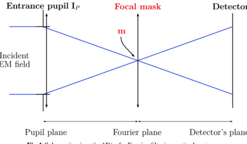
Fourier-based Wave front sensors1and coronagraphs both use optical Fourier filtering. Such a technique allows, thanks
to a mask placed in a focal plane, to handle the light in its spatial frequencies space (Fig. 1). In coronagraphy, these masks are designed to reject light while in wave front sensing they are built to convert phase fluctuations into intensity fluctuations. Some coronagraph masks may be turned into wave front sensing masks by minor modification. For
Fig 1 Schematic view (in 1D) of a Fourier filtering optical system.
instance, the Roddier & Roddier coronagraph2 and the Zernike WFS3,4 both use a mask which has a small circular
well in its midst. For an optical system working at the wavelength λ, the depth of this well equals to λ{2 in the coronagraph configuration while it is λ{4 for the Zernike sensor. Physically, the depth λ{2 implies a π phase shift between the fields inside and outside the central well: they are in opposition of phase. This fact induces the destructive interference which are required in coronagraphy. For the Zernike WFS, the phase shift equals to π{2; fields are now in phase quadrature.
2 The four quadrants wave front sensors class
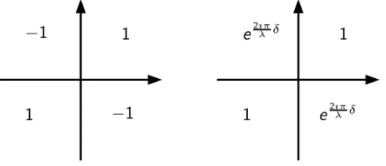
We propose here to extent this idea to another coronagraph called the Four Quadrants Phase Mask.5 Its mask has
a cartesian structure: the focal (or Fourier) plane is divided into 4-quadrants around the origin. In the coronagraph configuration, each quadrant is π phase-shifted with its two neighbors (left insert of Fig.2). We introduce in this paper a class of masks which have the same geometrical structure but with a shift not equal to π; namely, their differential
piston δ will have an arbitrary value between ´λ{2 and λ{2 (right insert of Fig. 2). The purpose of this article is to study the mathematical properties of these new optical objects and to examine their performance criteria in a wave front sensing context.
Fig 2 Transparency functions of the coronograph FQPM (left) and its generalization to an arbitrary differential piston δ (right).
The propagation through an optical Fourier filtering system using a four quadrants mask with an arbitrary differ-ential piston can be described by a linear operator W which gives the electric field in the detector plane depending on the incident electric field
W “ eıπλδ „ cosˆ πδ λ ˙ I ` ı sinˆ πδ λ ˙ H . (1)
Here I represents the identity operator1and H the 2D Hilbert transform along x and y axis Hrf s px, yq “ 1 π2 p.v. ż R2 dx1dy1 f px1, y1q px ´ x1qpy ´ y1q, (2) where p.v. indicates the principal value meaning. It is worth noticing that this operator is involutive and conserves the energy, i.e., the L2-norm. We observe that the field operator W in Eq. (1) contains two terms, the first one reproduces the incoming field while the second one provides its 2D Hilbert transform. The differential piston δ acts as a cursor between the two contributions. For δ “ 0 the masks are pointless since the propagator operator only contains the identity operator. The coronagraph case δ “ λ{2 gives a pure 2D Hilbert transform. Finally, if δ “ ˘λ{4, there is a perfect energy equipartition between the two terms.
In a wave front sensing context, we write the incident field as IPeıφ where IP is the indicator function of the entrance pupil and φ the phase-to-be-measured. For the sake of simplicity, the flux is considered unitary. The detector intensity Ipφq equals to the square modulus of the field in the detector plane
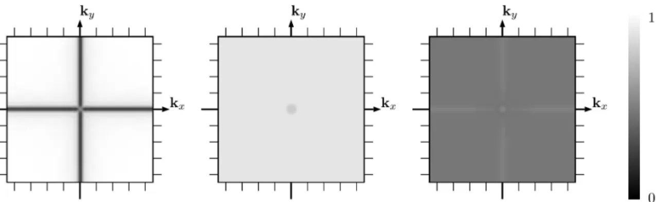
Ipφq “ ˇˇW“IPeıφ ‰ˇ ˇ 2 (3) “ sinˆ 2π λδ ˙ Im“pIPe´ıφqHrIPeıφs ‰ ` sin2ˆ πδ λ ˙ |HrIPeıφs|2` cos2 ˆ πδ λ ˙ I2P. (4) This intensity is crucial in two aspects. Firstly, it corresponds to the image that a phase reconstructor has to invert to estimate φ. Secondly, it gives the energy distribution that a Lyot’s stop6has to filter to make the light rejection efficient for coronagraphy. Such a fact becomes clearer when looking at the detector intensity for a flat incoming wave front, i.e., when φ equals to 0
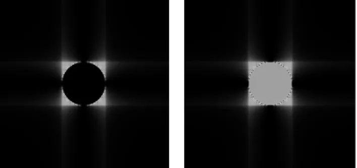
Ipφ “ 0q “ cos2ˆ πδ λ ˙ I2P` sin2ˆ πδ λ ˙ HrIPs2. (5) Indeed, we observe that in the coronagraph case (left insert of Fig.3), the energy location corresponds to the 2D Hilbert transform of the pupil while the cosine term is null. It is not surprising since we know that the Hilbert transform of a function has significant values where the function highly evolves, i.e., at the edge of the pupil. This is the reason why the FQPM is effective to reject light. Note that in Adaptive Optics (AO) the term Ip0q is also considered as a reference intensity to which a closed AO loop will try to maintain the detector intensity as close as possible. We give on the right insert of Fig.3this reference intensity for the case δ “ λ{4.
1Actually it is not rigorously the identity but the reverse operator: for the sake of clarity, we have ignored that the whole Fourier filtering system
Fig 3 Intensity on the detector for a circular pupil and a null incoming phase. Left: coronagraph case δ “ λ{2. Right: energy equipartition case δ “ λ{4.
From now on, we focus on wave front sensing. We first look for the mask among the four quadrants class which op-timizes the phase information coding. Then, we compare this optimal sensor to existing wave front sensors following usual AO performance criteria. First and foremost, we precise that we assume the AO control to apply linear recon-structors. In that context, finding the optimal sensor consists in maximizing the sensor sensitivity.1 Mathematically,
we therefore want to increase the φ-linear dependency of the intensity as much as possible. To do so, we decompose the intensity Ipφq using a Taylor’s development1around a reference phase Φ
rwhich serves as the operating point of the sensor.
Ipφq “ Iconstant` Ilinearpφq ` Iquadraticpφq ` ..., (6) where Iconstantequals to IpΦrq and does not depend on the phase φ. Ilinearcorresponds to the perfectly linear behavior of the sensor around the reference phase. It equals the Fr´echet derivative of the intensity around Φrin direction φ (for more details see the appendix 1). Iquadraticis the first non-linear phase-dependency. When assuming that the sensor is working around zero, i.e., Φr“ 0 we obtain
Ilinearpφq “sin
ˆ 2π λδ
˙
“HrIPsIPφ ´ HrIPφsIP ‰ , (7) Iquadraticpφq “sin2 ´π λδ ¯
“HrIPφs2´ HrIPsHrIPφs ‰
. (8)
These quantities have a similar structure: scalar termsonly depending on the differential piston δ and 2D terms
involving Hilbert transforms of the phase and the pupil. This pronounced decomposition is not systematic at all. The fact that the parameter δ has no influence on the spatial structure of the response to φ is an unexpected and very interesting characteristic of the FQPM class.
For the linear term some remarkable properties can be found. The first one is about its support. Indeed, Eq. (7) shows that it exactly corresponds to the pupil support. In other words, there is no linear information outside the pupil. Secondly, we observe that the scalar term is maximum when the differential piston ensures the energy equipartition between the real and imaginary parts of the propagation operators, i.e., δ “ ˘λ{4. Physically, this piston provides, as for the Zernike WFS, a ˘π{2 shift between the different parts of the focal plane tessellation. Such a result is in perfect agreement with the phase contrast method introduced in reference3. Note that in the coronagraph case δ “ λ{2, the linear term is rigorously null.
The quadratic term, as all non-linear terms, is for the AO control using linear reconstructors a perturbation which has to be kept as small as possible. Its size largely determines the linearity (or dynamic) range of the sensor.1 Unfor-tunately, Eq. (8) shows that this term only equals to zero for the pointless mask δ “ 0. In other words, it is impossible by using Fourier filtering and four quadrants masks (right insert of Fig. 2) to sense the wave front without having simultaneously a non-linear phase dependency. (Note, however, that linearity can be improved by the use of a 2 paths optical device, for more details see appendix 2.) From this discussion, we finally understand that the differential piston is also a cursor to adjust the sensitivity regarding to the linearity range of the WFS. Note, that these developments are valid for the Zernike WFS as well.
3 An optimum configuration
In what follows, we will focus on the mask with δ “ λ{4 which provides the energy equipartition. We call the associated WFS the ıQuad WFS. The notation Quad refers to the cartesian tessellation of the focal plane whereas the
ı emphasizes the transformation of the coronagraph FQPM transparency function (with its 1 and -1 coefficients; left insert of Fig.2) into the ıQuad WFS’s one (coefficients of the right insert of Fig.2equal to 1 and ı if δ “ λ{4).
Let us now compare the ıQuad WFS to two Fourier-based wave front sensors used in Adaptive Optics, namely the Zernike WFS4and the 4-sided non-modulated Pyramid WFS.7We precise that we assume the angle of the pyramidal prism to be large enough in order to completely separate the pupil images.
The first performance criterion is related to the number of the detector pixels required to code phase information. This aspect can be tackled in two ways. The first one is based on geometrical optics and considers that relevant phase information lies only inside pupil images. In that case, Zernike and ıQuad wave front sensors need 4 times less pixels than the Pyramid WFS to reach the same amount of information which is a huge gain in terms of data to process. Note that this factor 4 is decreasing toward 1 when using a flattened Pyramid WFS,8i.e., a pyramid mask with a small
apex angle which induces an overlap of the pupil images. The second approach is based on the study of the linear intensity. Indeed, this quantity is the main contributor for the numerical phase reconstructor to estimate the phase. As a consequence, in order to perform ultimate AO correction we want to make optimal use of sensor pixels being in the linear intensity support. We observe thanks to Eq. (7) that the intensity support itself exactly corresponds to the geometrical pupil image for the ıQuad WFS. Such a fact is also true for the Zernike WFS. In contrast, it appears that there is linear information outside the 4 pupil images for the Pyramid WFS. In other words, the whole detector has to be taken into account for this sensor. Thus, the Pyramid WFS requires even more than 4 times the number of pixels needed to sense the wave front with a Zernike or ıQuad WFS making the latter sensors efficient in terms of detector size.
We are now interested in the chromatic behavior of the ıQuad. As for the coronagraph FQPM, the ıQuad can be optimized for a specific wavelength only, meaning that the maximum of sensitivity will be obtained when the source’s wavelength equals to the mask’s optimization wavelength. Nevertheless, we observe thanks to Eq. (7) that the spatial structure of the response does not depend on the wavelength. This one has only an impact on a global scalar level. Physically, it comes from the fact that the four quadrants masks have, with their cartesian tessellation, a scale invariant geometry. It is not true for the Zernike WFS which has, due to the finite size of its central well, a spatial structure of its response changing with the wavelength. This remarkable property implies, for instance, that a calibration matrix built at a certain wavelength may be used to sense the phase with another source (or even with a polychromatic one). It will be only a matter of scalar gain. It is worth noticing that the ıQuad WFS shares this property with the non-modulated Pyramid WFS.
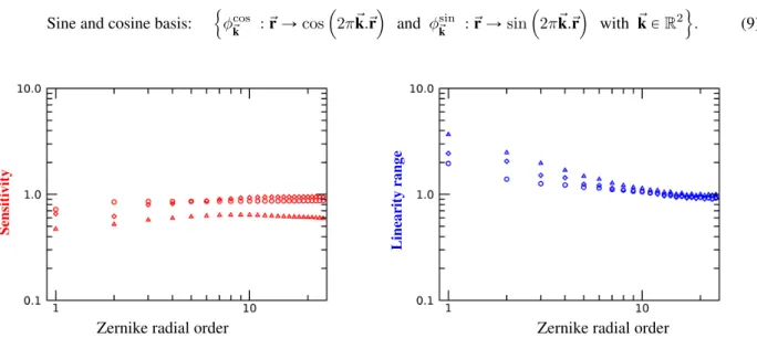
We now study two fundamental performance criteria, namely sensitivity and linearity range and compare those for the different sensor types. The criteria are computed following the method of reference1and represented with respect to the Zernike polynomials in Fig.4and to the sine and cosine basis (i.e., the spatial frequencies) in Fig.5
Sine and cosine basis: !
φcos~
k : ~r Ñ cos ´
2π~k.~r¯ and φ~sink : ~r Ñ sin ´ 2π~k.~r¯ with ~k P R2). (9) Sensiti vity Linearity range
Zernike radial order Zernike radial order
Fig 4 Sensitivity(left) andlinearity range(right) with respect to the 25 first Zernike radial orders (which corresponds to around 300 Zernike polynomials). 4 Pyramid. ` ıQuad. ˝ Zernike.
In terms of linearity range (blue curves), the three wave front sensors are almost equivalent for the high frequencies. Main differences concern low frequencies, whereby the ıQuad lies between the Pyramid and the Zernike performance
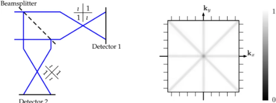
Fig 5 Sensitivity with respect to the phase spatial frequencies ~k “(kx, ky) for the ıQuad (left), Zernike (middle) and Pyramid (right) wave front
sensors.
curves. Regarding the sensitivity (red curves), the ıQuad surpasses the non-modulated Pyramid WFS by a factor of approximately 2 on the whole frequency range. It has similar performance as the Zernike WFS: the ıQuad is slightly better for the high spatial frequencies whereas the Zernike is a bit more sensitive for the low frequencies. The largest sensitivity difference concerns the second radial order which contains the focus and the two astigmatisms aberrations. Such a reduced sensitivity is due to the fact that the ıQuad sensor has difficulty to code the vertical astigmatism Z22 (left insert of Fig. 6). Quantitatively, the ıQuad’s sensitivity with respect to this mode is almost 30 lower than the Zernike’s sensitivity. The physical reason of this very low sensitivity is a matter of symmetry. Indeed, when looking at
Fig 6 Left: structure of the badly-seen mode computed thanks to a singular value decomposition. Right: 2D Fourier transform of this mode.
the Fourier transform of the badly-seen mode (right insert of Fig.6), we observe that its structure is turned through 45 degrees with respect to the ıQuad mask geometry. This implies destructive interference which annihilates the linear response of the sensor to this mode. When looking at the 2D sensitivity with respect to the spatial frequencies (left insert of Fig. 5), we observe that Z2
2 is not the only mode which is incorrectly seen by the ıQuad WFS. The black cross indicates that phases which only contain pure x or y frequencies (in other words, frequencies which lie on the edge of the cartesian tessellation) are badly seen by the sensor.
Such a geometrical consideration implies that a Fourier-based WFS using a turned through 45 degrees ıQuad mask is able to correctly measure the previous unseen frequencies. However, it cannot properly see the diagonals spatial frequencies. Hence, a 2-paths optical system using simultaneously two ıQuad sensors with two different mask’s orientations has no badly-seen spatial frequencies (see Fig.7).
The last part of this paper is dedicated to a curious mathematical property of the ıQuad WFS. Its linear intensity turns out to be very close to the slopes maps9 of the Pyramid WFS. Slopes maps result from a numerical processing performed on the detector intensity of the Pyramid WFS. They consist in two combinations of the 4 pupil images and allow to compress the Pyramid WFS signal in two pupil images only but also to understand them in terms of phase derivatives along x and y-axis. Assuming a reflective Pyramid working in its linearity domain, the slopes maps are approximated by Sx`φ˘px, yq “ IPpx, yq π ż P φpx, yq ´ φpx1, yq x ´ x1 dx 1, (10)
Fig 7 Left: Optical configuration of the 2-paths ıQuad WFS. Right: Sensitivity with respect to the phase spatial frequencies. Sy`φ˘px, yq “ IPpx, yq π ż P φpx, yq ´ φpx, y1q y ´ y1 dy 1. (11)
We can describe these quantities as integrated difference quotient along x and y directions. That is why slopes maps are close to the derivatives of the wave front. Nevertheless, they are not rigorously phase derivatives since the 1D Hilbert transform along x (resp. y) plays the most significant role in the Sx(resp. Sy) expression. We now compare Eqs. (10) and (11) to the linear intensity of the ıQuad WFS (7). The latter becomes, if we develop it with respect to spatial coordinates, Ilinear`φ˘px, yq “ IPpx, yq π2 ż P φpx, yq ´ φpx1, y1q px ´ x1qpy ´ y1q dx 1dy1. (12) Thus, it appears that the ıQuad signal is a condensed version of the two Pyramid slopes maps. Indeed, this sensor optically computes in one pupil image only, the x and y Hilbert transforms of the phase. Physically, this unexpected parallel between the ıQuad and the Pyramid WFS is essentially related to the fact that they both use a cartesian tessellation of the focal plane. No matter how the phase information is shaped – by doing optical interference with the differential piston of the ıQuad or by splitting the spatial frequencies with prisms to then numerically processing them with the Pyramid WFS – the involved mathematical operators depend on the way we subdivide the focal plane.
The great similarity between the ıQuad and Pyramid WFS slopes maps signals is profitable in many ways. Firstly, there already exist a lot of model-based reconstruction algorithms10 dedicated to the Pyramid WFS which can be
extended to build effective reconstructors for the ıQuad WFS. Moreover, this numerical implementation will be facil-itated by the fact that the linear intensity operator of the ıQuad (12) turns out to be self-adjoint (for more details, see appendix 1); this is a very convenient property for some iterative mathematical algorithms as, e.g., the linear Landwe-ber iteration.10 Finally, this sensor, which is mathematically much more intelligible than the real Pyramid WFS (it does not require any assumption on the pyramid angle for instance) can be seen as a theoretical extension of the Pyramid WFS.
4 Conclusion
In this paper, we introduced a new class of Fourier-based wave front sensors derived from the FQPM coronagraph. Their filtering mask uses a cartesian tessellation of the focal plane with a unique parameter: the differential piston between quadrants. This degree of freedom allowed to find an optimal WFS regarding to the sensitivity performance, that we called the ıQuad WFS. Its differential piston ensures that the fields of each neighbor quadrant are in quadrature of phase. This result proves that the shift from the coronagraph FQPM to the ıQuad WFS rigorously mimics the shift from the Roddier & Roddier coronagraph to the Zernike WFS. We then studied the performance criterion of the ıQuad and observed that this sensor was
• efficient in terms of the number of pixels required to sense the wave front, • less chromatic than the Zernike WFS and
• competitive in terms of sensitivity and linearity range.
Despite the badly-seen frequencies of the ıQuad, we saw that a two optical paths solution using two ıQuad masks with different orientations could solve this problem. In conclusion, rather than being a practical sensor, the single
path ıQuad may be viewed like a theoretical object which has an elegant mathematical formulation and also builds a bridge between the Pyramid (because of the unexpected similarity between ıQuad output and the slopes maps) and the Zernike wave front sensors (since the ıQuad is based on the phase contrast method).
Acknowledgments. Noah Schwartz (UK Astronomy Technology Centre, Edinburgh) is acknowledged for fruitful discussion.
Funding. Laboratoire d’Astrophysique de Marseille (LAM) (VASCO Research Project); French Aerospace Lab (ONERA); ANR-18-CE31-0018-01-WOLF; ANR Tremplin-ERC 16-TERC-0008-01); ANR A*MIDEX (ANR-11-IDEX-0001- 02); Horizon 2020 (ASHRA 730890); LABEX FOCUS; Austrian Science Fund (F68-N36, project 5); Austrian Federal Ministry of Science and Research (HRSM).
Appendices
Appendix 1: Gˆateaux derivatives of the ıQuad WFS
In this appendix, we prove that the Gˆateaux derivative of the ıQuad intensity around any reference phase Φrequals to
`IpΦrq1˘φpx, yq “ IPpx, yq π2 ż P dx1dy1rφpx, yq ´ φpx 1, y1qs cosrΦ rpx, yq ´ Φrpx1, y1qs px ´ x1qpy ´ y1q ´1 2 ż P ż P dx1dy1dx2dy2rφpx 1, y1q ´ φpx2, y2qs sinrΦ rpx1, y1q ´ Φrpx2, y2qs π4px ´ x1qpy ´ y1qpx ´ x2qpy ´ y2q (13) and show that it allows to get the linear intensity Ilineargiven in Eq. (7).
Proof. We first expand the detector intensity (4) regarding to the spatial coordinates
I`φ˘px, yq “ IPpx, yq π2 ż P dx1dy1sinrφpx, yq ´ φpx 1, y1 qs px ´ x1qpy ´ y1q ` I2Ppx, yq ` ż P ż P dx1dy1dx2dy2 cosrφpx 1, y1q ´ φpx2, y2qs π4px ´ x1qpy ´ y1qpx ´ x2qpy ´ y2q, in which it was assumed that δ “ λ{4. We may observe that this formula corresponds to a decomposition into an odd and an even part regarding to the phase: Ipφq “ Ioddpφq ` Ievenpφq with
Iodd`φ˘px, yq :“ IPpx, yq π2 ż P dx1dy1sinrφpx, yq ´ φpx 1, y1qs px ´ x1qpy ´ y1q Ieven`φ˘px, yq :“ 1 2 ˆ I2Ppx, yq ` ż P ż P dx1dy1dx2dy2 cosrφpx1, y1q ´ φpx2, y2qs π4px ´ x1qpy ´ y1qpx ´ x2qpy ´ y2q ˙ .
Utilizing similar to reference11Taylor’s theorem with the Lagrange form of the remainder for the representation of sine and cosine the Gˆateaux derivatives of these odd and even intensities around the reference phase Φr are per definition computed as `IoddpΦrq1˘ φ px, yq “ lim tÑ0 pIoddpΦr` tφqq px, yq ´ pIoddpΦrqq px, yq t “ lim tÑ0 IPpx, yq π2 ż P dx1dy1sin“Φrpx, yq ` tφpx, yq ´ Φrpx 1, y1 q ´ tφpx1, y1 q‰´ sin“Φrpx, yq ´ Φrpx1, y1q ‰ tpx ´ x1qpy ´ y1q “ lim tÑ0 IPpx, yq π2 ż P dx1dy1sin 1“Φ rpx, yq ´ Φrpx1, y1q‰ “tφpx, yq ´ tφpx1, y1q ‰ ` O`t2φ2˘ tpx ´ x1qpy ´ y1q “ IPpx, yq π2 ż P dx1dy1“φpx, yq ´ φpx 1, y1q‰ cos “Φ rpx, yq ´ Φrpx1, y1q ‰ px ´ x1qpy ´ y1q ,
`IevenpΦrq1˘ φ px, yq “ lim tÑ0 pIevenpΦr` tφqq px, yq ´ pIevenpΦrqq px, yq t “ lim tÑ0 1 2 ˜ I2Ppx, yq ` ż P ż P dx1dy1dx2dy2cos“Φrpx 1, y1q ` tφpx1, y1q ´ Φ rpx2, y2q ´ tφpx2, y2q ‰ tπ4px ´ x1qpy ´ y1qpx ´ x2qpy ´ y2q ¸ ´1 2 ˜ I2Ppx, yq ` ż P ż P dx1dy1dx2dy2 cos“Φrpx 1, y1 q ´ Φrpx2, y2q ‰ tπ4px ´ x1qpy ´ y1qpx ´ x2qpy ´ y2q ¸ “ lim tÑ0 1 2 ż P ż P dx1dy1dx2dy2cos 1“Φ rpx1, y1q ´ Φrpx2, y2q‰ “tφpx1, y1q ´ tφpx2, y2q ‰ ` O`t2φ2˘ tπ4px ´ x1qpy ´ y1qpx ´ x2qpy ´ y2q “ ´1 2 ż P ż P dx1dy1dx2dy2“φpx 1 , y1q ´ φpx2, y2q‰ sin “Φrpx1, y1q ´ Φrpx2, y2q ‰ π4px ´ x1qpy ´ y1qpx ´ x2qpy ´ y2q .
The claim follows with I “ Iodd` Ieven.
Similar to reference11one can show that the Gˆateaux derivative of the ıQuad sensor equals the Fr´echet derivative. Note that assuming Φris the null phase in Eq. (13) allows then to get the ıQuad linear intensity (12).
We are now interested in the adjoint of the Fr´echet derivative which is a pivotal quantity in many iterative algorithms used to reconstruct the phase.10 The L
2`R2 ˘
-adjoint operator pIpΦrq1q˚ : L2`R2 ˘
Ñ L2`R2 ˘
of the ıQuad sensor Fr´echet derivative in Φris represented by
`IpΦrq1 ˘˚ φ px, yq “ IPpx, yq π2 ż P dx1dy1rφpx, yq ´ φpx 1, y1qs cos rΦ rpx, yq ´ Φrpx1, y1qs px ´ x1qpy ´ y1q ´ ż P ż P dx1dy1dx2dy2 φpx1, y1q sin rΦrpx, yq ´ Φrpx2, y2qs π4px ´ x1qpy ´ y1qpx1´ x2qpy1´ y2q. (14)
Proof. For the evaluation of the adjoints, we divide the Fr´echet derivative into four parts by IpΦrq1“ IoddpΦrq1` IevenpΦrq1,
I1
oddpΦrq “ Iodd,1pΦrq ´ Iodd,2pΦrq, I1
evenpΦrq “ Ieven,1pΦrq ´ Ieven,2pΦrq with pIodd,1pΦrqq φ px, yq :“ IPpx, yq π2 ż P dx1dy1φpx, yq cos rΦrpx, yq ´ Φrpx1, y1qs px ´ x1qpy ´ y1q , pIodd,2pΦrqq φ px, yq :“ IPpx, yq π2 ż P dx1dy1φpx 1, y1q cos rΦ rpx, yq ´ Φrpx1, y1qs px ´ x1qpy ´ y1q , pIeven,1pΦrqq φ px, yq :“ ´ 1 2 ż P ż P dx1dy1dx2dy2φpx 1, y1q sin rΦ rpx1, y1q ´ Φrpx2, y2qs π4px ´ x1qpy ´ y1qpx ´ x2qpy ´ y2q, pIeven,2pΦrqq φ px, yq :“ ´ 1 2 ż P ż P dx1dy1dx2dy2φpx 2, y2q sin rΦ rpx1, y1q ´ Φrpx2, y2qs π4px ´ x1qpy ´ y1qpx ´ x2qpy ´ y2q . For φ, ψ P L2`R2 ˘
with support on the telescope pupil P we consider xpIodd,1pΦrqq φ, ψyL2pR2q“ xpIodd,1pΦrqq φ, ψyL2pP q
“ ż P dxdy„ IPpx, yq π2 ż P dx1dy1φpx, yq cos rΦrpx, yq ´ Φrpx 1, y1qs px ´ x1qpy ´ y1q ψ px, yq “ ż P dxdy φ px, yq 1 π2 ż P dx1dy1ψpx, yq cos rΦrpx, yq ´ Φrpx1, y1qs px ´ x1qpy ´ y1q “ xφ, pIodd,1pΦrqq˚ψyL2pP q “ xφ, pIodd,1pΦrqq˚ψyL2pR2q, which results in ` pIodd,1pΦrqq˚ψ ˘ px, yq “ IPpx, yq π2 ż P dx1dy1ψpx, yq cos rΦrpx, yq ´ Φrpx1, y1qs px ´ x1qpy ´ y1q ,
i.e., Iodd,1is self-adjoint. Moreover,
xpIodd,2pΦrqq φ, ψyL2pR2q“ xpIodd,2pΦrqq φ, ψyL2pP q
“ ż P dxdy„ IPpx, yq π2 ż P dx1dy1φpx 1, y1q cos rΦ rpx, yq ´ Φrpx1, y1qs px ´ x1qpy ´ y1q ψ px, yq “ ż P dx1dy1φ`x1, y1˘ 1 π2 ż P dxdyψpx, yq cos rΦrpx, yq ´ Φrpx 1, y1qs px ´ x1qpy ´ y1q “ ż P dxdy φ px, yq 1 π2 ż P dx1dy1ψpx 1, y1q cos rΦ rpx, yq ´ Φrpx1, y1qs px1´ xqpy1´ yq “ xφ, pIodd,2pΦrqq˚ψyL2pP q “ xφ, pIodd,2pΦrqq˚ψyL2pR2q
with (as cosine is even) ` pIodd,2pΦrqq˚ψ ˘ px, yq “ IPpx, yq π2 ż P dx1dy1ψpx 1, y1q cos rΦ rpx, yq ´ Φrpx1, y1qs px ´ x1qpy ´ y1q , i.e., Iodd,2is self-adjoint as well. Similarly, for IevenpΦrq1we calculate
xpIeven,1pΦrqq φ, ψyL2pR2q“ xpIeven,1pΦrqq φ, ψyL2pP q
“ ´ ż P dxdy„ 1 2 ż P ż P dx1dy1dx2dy2φpx 1, y1q sin rΦ rpx1, y1q ´ Φrpx2, y2qs π4px ´ x1qpy ´ y1qpx ´ x2qpy ´ y2q ψ px, yq “ ´ ż P dx1dy1φ`x1, y1˘ 1 2 ż P ż P dxdydx2dy2ψpx, yq sin rΦrpx 1, y1 q ´ Φrpx2, y2qs π4px ´ x1qpy ´ y1qpx ´ x2qpy ´ y2q “ ´ ż P dxdy φ px, yq1 2 ż P ż P dx1dy1dx2dy2 ψpx 1, y1q sin rΦ rpx, yq ´ Φrpx2, y2qs π4px1´ xqpy1´ yqpx1´ x2qpy1´ y2q “ xφ, pIeven,1pΦrqq˚ψyL2pP q “ xφ, pIeven,1pΦrqq˚ψyL2pR2q with ` pIeven,1pΦrqq˚ψ ˘ px, yq “ ´1 2 ż P ż P dx1dy1dx2dy2 ψpx 1, y1q sin rΦ rpx, yq ´ Φrpx2, y2qs π4px ´ x1qpy ´ y1qpx1´ x2qpy1´ y2q and
xpIeven,2pΦrqq φ, ψyL2pR2q“ xpIeven,2pΦrqq φ, ψyL2pP q “ ´ ż P dxdy„ 1 2 ż P ż P dx1dy1dx2dy2φpx 2, y2q sin rΦ rpx1, y1q ´ Φrpx2, y2qs π4px ´ x1qpy ´ y1qpx ´ x2qpy ´ y2q ψ px, yq “ ´ ż P dx2dy2φ`x2, y2˘ 1 2 ż P ż P dx1dy1dxdyψpx, yq sin rΦrpx 1, y1 q ´ Φrpx2, y2qs π4px ´ x1qpy ´ y1qpx ´ x2qpy ´ y2q “ ´ ż P dxdy φ px, yq1 2 ż P ż P dx1dy1dx2dy2 ψpx 2, y2q sin rΦ rpx1, y1q ´ Φrpx, yqs π4px2´ x1qpy2´ y1qpx2´ xqpy2´ yq “ xφ, pIeven,2pΦrqq˚ψyL2pP q “ xφ, pIeven,2pΦrqq˚ψyL2pR2q, which results in ` pIeven,2pΦrqq˚ψ ˘ px, yq “ ´1 2 ż P ż P dx1dy1dx2dy2 ψpx 2, y2q sin rΦ rpx1, y1q ´ Φrpx, yqs π4px ´ x2qpy ´ y2qpx1´ x2qpy1´ y2q “ ´1 2 ż P ż P dx1dy1dx2dy2 ψpx 1, y1q sin rΦ rpx2, y2q ´ Φrpx, yqs π4px ´ x1qpy ´ y1qpx1´ x2qpy1´ y2q “ 1 2 ż P ż P dx1dy1dx2dy2 ψpx1, y1q sin rΦrpx, yq ´ Φrpx2, y2qs π4px ´ x1qpy ´ y1qpx1´ x2qpy1´ y2q.
Hence, the adjoint of the Fr´echet derivative of the ıQuad sensor is given by `IpΦrq1
˘˚
φ px, yq “ pIodd,1pΦrqq˚φ px, yq ´ pIodd,2pΦrqq˚φ px, yq ` pIeven,1pΦrqq˚φ px, yq ´ pIeven,2pΦrqq˚φ px, yq “ IPpx, yq π2 ż P dx1dy1rφpx, yq ´ φpx 1, y1 qs cos rΦrpx, yq ´ Φrpx1, y1qs px ´ x1qpy ´ y1q ´1 2 ż P ż P dx1dy1dx2dy2 φpx 1, y1q sin rΦ rpx, yq ´ Φrpx2, y2qs π4px ´ x1qpy ´ y1qpx1´ x2qpy1´ y2q ´1 2 ż P ż P dx1dy1dx2dy2 φpx 1, y1q sin rΦ rpx, yq ´ Φrpx2, y2qs π4px ´ x1qpy ´ y1qpx1´ x2qpy1´ y2q “ IPpx, yq π2 ż P dx1dy1rφpx, yq ´ φpx1, y1qs cos rΦrpx, yq ´ Φrpx1, y1qs px ´ x1qpy ´ y1q ´ ż P ż P dx1dy1dx2dy2 φpx 1, y1q sin rΦ rpx, yq ´ Φrpx2, y2qs π4px ´ x1qpy ´ y1qpx1´ x2qpy1´ y2q, which proofs the claim.
Eq. (14) allows then to calculate the adjoint operator of the linear intensity around the null phase Φr “ 0. We get that the adjoint operator pIlinearq˚ : L2`R2
˘
Ñ L2`R2 ˘
of the linear ıQuad sensor around the zero phase is represented by pIlinearq˚φpx, yq “`Ip0q1 ˘˚ φpx, yq “ IPpx, yq π2 ż P dx1dy1φpx, yq ´ φpx 1, y1q px ´ x1qpy ´ y1q , (15) i.e., the operator is self-adjoint because of Ilinear“ pIlinearq˚as a comparison of Eq. (12) and Eq. (15) shows. This re-markable property is unprecedented in the Fourier filtering wave front sensors world and makes the ıQuad particularly appropriate to model-based phase reconstructors.
Appendix 2: Improving the linearity
In this second appendix, we show how it is possible to improve the linearity of the ıQuad by using a 2-paths optical design. The idea consists in dividing the field into two fields which are Fourier filtered by two different masks: the ıQuad mask and its conjugate, the ´ıQuad, see Fig.8.
Fig 8 Optical system of the Odd ıQuad.
The optical propagators of the two paths are W1“ I ´ ıH ? 2 W2“ I ` ıH ? 2 . (16)
The incoming field amplitude is divided by?2 by the beamsplitter which gives two intensities:
I1pφq “ ˇ ˇ ˇ ˇ W1 „ IPeıφ ? 2 ˇ ˇ ˇ ˇ 2 I2pφq “ ˇ ˇ ˇ ˇ W2 „ IPeıφ ? 2 ˇ ˇ ˇ ˇ 2 . (17)
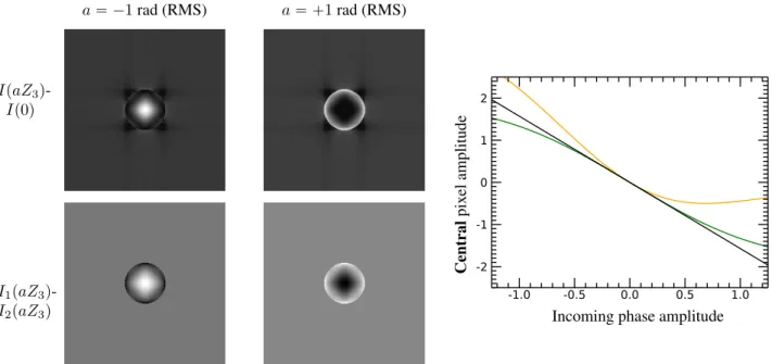
The WFS’s output is defined as the difference between these two intensities: dIpφq “ I1pφq ´ I2pφq, (18) which results in dI`φ˘px, yq “ IPpx, yq π2 ż P dx1dy1sinrφpx 1, y1q ´ φpx, yqs px ´ x1qpy ´ y1q (19) This optical configuration allows to cancel even intensity in the ıQuad intensity. In particular, the first non-linear term is the cubic one and not, as usually, the quadratic one. Such a fact implies an improvement of the sensor linearity (see Fig.9). IpaZ3 q-Ip0q I1paZ3 q-I2paZ3q a “ ´1 rad (RMS) a “ `1 rad (RMS) Central pix el amplitude -1.0 -0.5 0.0 0.5 1.0 Incoming phase amplitude -2 -1 0 1 2 Meta-pixel amplitude
Incoming phase amplitude
Fig 9 Left pictures: Output maps for the 1-path (top) and 2-paths (bottom) iQuad when ˘1 rad RMS Focus (Z3) goes through the WFS. 1-path is
neither odd, nor even. 2-paths is odd with respect to the phase. Moreover, it is worth noticing that there is no signal outside the pupil geometric image for the 2-paths device. Right insert: relation between the amplitude of an incoming phase and the amplitude of the central pixel of the WFS’s output for the1-pathand the2-pathsıQuads. The same tangent at the origin indicates an identical sensitivity (black curve). Moreover, we observe that the 2-paths system provides a symmetrical response which is not the case of the 1-path. Such a fact implies a better linearity for the 2-paths ıQuad than the classical one.
References
1 O. Fauvarque,“General formalism for Fourier-based wave front sensing,” Optica 3, 1440–1452 (2016).
2 F. Roddier, and C. Roddier “Stellar Coronagraph with Phase Mask,” Astronomical Society of the Pacific 109, 815–820 (1997).
3 F. Zernike, “Diffraction theory of the knife-edge test and its improved form, the phase-contrast method,” Royal Astronomical Society 94, 377–383 (1934).
4 M. N’Diaye, K. Dohlen, T. Fusco, and B. Paul, “Calibration of quasi-static aberrations in exoplanet direct-imaging instruments with a Zernike phase-mask sensor,” Astronomy and Astrophysics 555, A94 (2013).
5 D. Rouan, “The Four-Quadrant Phase-Mask Coronagraph,” Astronomical Society of the Pacific 112, 1479–1486 (2000).
6 B. Lyot, “Photographie de la couronne solaire en dehors des eclipses,” Compte-rendu Academie Scientifique de Paris 193-1169, 48 (1931).
7 R. Ragazzoni, “Pupil plane wavefront sensing with an oscillating prism,” Journal of Modern Optics 43, 289–293 (1996).
8 O. Fauvarque, B. Neichel, T. Fusco, and J.-F. Sauvage, “Variation around a pyramid theme : optical recombination and optimal use of photons,” Optics Letters 15, 3528–3531 (2015).
9 C. V´erinaud, “On the nature of the measurements provided by a pyramid wave-front sensor,” Optics Communica-tions 233, 27–38 (2004).
10 V. Hutterer, I. Shatokhina, A. Obereder, and R. Ramlau, “Wavefront reconstruction for ELT-sized telescopes with pyramid wavefront sensors,” Proc. SPIE 1070344, (2018).
11 V. Hutterer, I. Shatokhina, and R. Ramlau, “Real-time Adaptive Optics with pyramid wavefront sensors: A theo-retical analysis of the pyramid sensor model,” Inverse Problems 35(4), 045007 (2019).