HAL Id: hal-01344078
https://hal.archives-ouvertes.fr/hal-01344078
Submitted on 11 Jul 2016
HAL is a multi-disciplinary open access
archive for the deposit and dissemination of
sci-entific research documents, whether they are
pub-lished or not. The documents may come from
teaching and research institutions in France or
abroad, or from public or private research centers.
L’archive ouverte pluridisciplinaire HAL, est
destinée au dépôt et à la diffusion de documents
scientifiques de niveau recherche, publiés ou non,
émanant des établissements d’enseignement et de
recherche français ou étrangers, des laboratoires
publics ou privés.
Improvement of the Embarrassingly Parallel Search for
Data Centers
Jean-Charles Régin, Mohamed Rezgui, Arnaud Malapert
To cite this version:
Jean-Charles Régin, Mohamed Rezgui, Arnaud Malapert. Improvement of the Embarrassingly Parallel
Search for Data Centers. CP 2014, Sep 2014, Lyon, France. �10.1007/978-3-319-10428-7_45�.
�hal-01344078�
Improvement of the Embarrassingly Parallel Search
for data centers
Jean-Charles R´egin??, Mohamed Rezgui∗∗, and Arnaud Malapert∗∗ Univ. Nice Sophia Antipolis, CNRS, I3S, UMR 7271, 06900 Sophia Antipolis, France
Abstract. We propose an adaptation of the Embarrassingly Parallel Search (EPS) method for data centers. EPS is a simple but efficient method for parallel solving of CSPs. EPS decomposes the problem in many distinct subproblems which are then solved independently by workers. EPS performed well on multi-cores ma-chines (40), but some issues arise when using more cores in a datacenter. Here, we identify the decomposition as the cause of the degradation and propose a par-allel decomposition to address this issue. Thanks to it, EPS gives almost linear speedup and outperforms work stealing by orders of magnitude using the Gecode solver.
1
Introduction
Several methods for parallelizing the search in constraint programming (CP) have been proposed. The most famous one is the work stealing [12,14,5,16,3,8]. This method uses the cooperation between computation units (workers) to divide the work dynamically during the resolution. Recently, [13] introduced a new approach named Embarrass-ingly Parallel Search (EPS), which has been shown competitive with the work stealing method.
The idea of EPS is to decompose statically the initial problem into a huge number of subproblems that are consistent with the propagation (i.e. running the propagation mechanism on them does not detect any inconsistency). These subproblems are added to a queue which is managed by a master. Then, each idle worker takes a subproblem from the queue and solves it. The process is repeated until all the subproblems have been solved. The assignment of the subproblems to workers is dynamic and there is no communication between the workers. EPS is based on the idea that if there is a large number of subproblems to solve then the resolution times of the workers will be balanced even if the resolution times of the subproblems are not.
In other words, load balancing is automatically obtained in a statistical sense. In-terestingly, experiments of [13] have shown that the number of subproblems does not depend on the initial problem but rather on the number of workers. Moreover, they have shown that a good decomposition has to generate about 30 subproblems per worker. Experiments have shown good results on a multi-cores machine (40 cores/workers).
??This work was granted access to the HPC and visualization resources of ”Centre de Calcul
Interactif” hosted by the University of Nice Sophia Antipolis. It was also partially supported by OSEO, with the project ISI ”Pajero”.
Preliminary experimental results of this method on a data center (512 cores/workers) have shown that the scalability of the overall resolution time without the decomposition is very good. However, the decomposition becomes more difficult and the relative part of the decomposition compared to the overall resolution time grows with the number of workers. There are several reasons for that. First, the number of subproblems that have to be generated grows linearly with the number of cores. Second, the overall resolution time diminishes when the number of workers is increased. At last, the decomposition of the EPS method as proposed in [13] is not efficiently parallelized. In this paper we propose to address this issue by designing an efficient parallel decomposition of the initial problem.
A naive decomposition in parallel has been proposed in [13]. It splits the initial problem into as many subproblems as there are workers and assigns a subproblem to each worker. Then, each worker decomposes its subproblem into 30 subproblems. This gains a factor of 2 or 3 in comparison with a sequential decomposition. This is enough when the number of workers is limited (40 for instance) but it is no longer an efficient method with hundreds of workers. The gain is limited because there is no reason to have equivalent subproblems to decompose. However, from this naive algorithm we learn several things:
1. the difference of total work (i.e. activity time in EPS) made by the workers de-creases when the number of subproblems inde-creases. This is not a linear relation. There is a huge difference between the activity time of the workers when there are less than 5 subproblems per worker. These differences decrease when there are more than 5 subproblems per worker.
2. a simple decomposition into subproblems that may be inconsistent causes quickly some issues because inconsistencies are detected very quickly.
3. splitting an initial problem into a small set of subproblems is fast compared to the overall decomposition time and compared to the overall resolution time.
From these observations we understand that we will have to find a compromise and we propose an iterative process decomposing the initial problem in 3 phases. In the first phase, we want to decompose it into only few subproblems because the relative cost is small even if we have an unbalanced workload. However, we should be careful with the first phase (i.e. starting with probably inconsistent subproblems) because it can have an impact on the performance. At last, the most important thing seems to generate 5 subproblems because we could restart from these subproblems to decompose more and such a decomposition should be reasonably well balanced.
Thus, we propose a method which has 3 main phases:
– An initial phase where we generate as quickly as possible one subproblem per worker.
– A main phase which aims at generating 5 subproblems per worker. Each subprob-lem is consistent with the propagation. This phase can be divided into several steps for reaching that goal while balancing the work among the workers.
– A final phase which consists of generating 30 subproblems per worker from the set of subproblems computed by the main phase.
The paper is organized as follows. First we recall some preliminaries. Next, we describe the existing decomposition and we present an efficient parallelization of the decomposition. Then, we give some experimental results. At last, we conclude.
2
Preliminaries
A worker is a computation unit. Most of the time, it corresponds to a core. We will consider that there are w workers. We present the two methods that we will compare.
2.1 Work stealing
The work stealing method was originally proposed in [2] and was first implemented in Lisp parallel machines [4]. It splits the problem dynamically during the resolution. The workers solve the subproblems and when a worker finishes a subproblem, it asks the other workers for more work. In general, it is carried out as follows: when a worker W does not have work, it asks another worker V to get some work. If V agrees to give some of its work, then its splits the current subproblem into two subproblems and gives one to W . We say that W ”steals” some work of V . If V does not agree to give some work to W , then W asks another worker U for some work until it gets some work or all workers have been solicited.
This method has been implemented in a lot of solvers (Comet [8] or ILOG Solver [12] for instance), and into several manners [14,5,16,3] depending on whether the work to be done is centralized or not, on the way the search tree is split, or on the communi-cation method between workers. Work stealing attempts to solve partially the balancing issue of the workload by decomposing dynamically the subproblems.
When a worker is starving, it should not steal easy problems, because it would ask work again almost instantly. It happens frequently at the end of the search when many workers have no subproblems to solve. Thus, there are a lot of unnecessary communi-cations. [11] proposes to use a threshold to avoid these unnecessary communications but its efficiency depends on the search space. Generally, this method scales well for a few workers but it is difficult to keep a linear speedup with a huge number of workers.
Some methods [15,5] attempt to increase the scalability. In [15], the authors propose a masters/workers approach. Each master has its own workers. The search space is divided between the different masters, then each master puts its attributed sub-trees in a work pool to dispatch to the workers. When a node of the sub-tree is detected that is a root of large sub-tree, the workers generate a large number of sub-trees and put them in a the work pool in order to have a better load balancing.
In [5], the authors experiment with up to 64 cores using a work stealing strategy. A master centralizes all pieces of information (bounds, solutions and requests). The master estimates which worker has the largest amount of work in order to give some work to an idle worker.
Another drawback is that the implementation of the work stealing is intrusive and is strongly dependent of the solver which requires to have a very good knowledge of the CP solver and to access to some internal functions. Some methods try to address this issue [7].
2.2 EPS
The Embarassingly Paralell Search (EPS) method has been defined in [13]. This method splits statically the initial problem into a large number of subproblems that are consis-tent with the propagation and puts them in a queue. Once this decomposition is over, the workers take dynamically the subproblems from the queue when they are idle. Pre-cisely, EPS relies on the following steps:
• it splits a problem into p subproblems such as p ≥ w and pushes them into the
queue.
• each worker takes dynamically a subproblem in the queue and solves it. • a master monitors the concurrent access of the queue.
• the resolution ends when all subproblems are solved.
For optimization problems, the master manages the value of the objective. When a worker takes a subproblem from the queue, it also takes the best objective value com-puted so far. And when a worker solves a subproblem it communicates to the worker the value of the objective function. Note that there is no other communication, that is when a worker finds a better solution, the other workers that are running cannot use it for improving their current resolution.
The reduction of communication is an advantage over the work stealing. Further-more, a resolution in parallel can be replayed by saving the order in which the subprob-lems have been executed. This costs almost nothing and helps a lot the debugging of applications.
2.3 Definitions
A constraint network CN = (X , D, C) is defined by:
• a set of n variables X = {x1, x2, . . . , xn}
• a set of n finite domains D = {D(x1), D(x2), . . . , D(xn)} with D(xi) the set of
possible values for the variable xi,
• a set of constraints between the variables C = {C1, C2, . . . , Ce}. A constraint Ci
is defined on a subset of variables XCi= {xi1, xi2, . . . , xij} of X with a subset of
Cartesian product D(xi1) × D(xi2) × . . . × D(xij), that states which combinations
of values of variables {xi1, xi2, . . . , xij} are compatible.
Each constraint Ci is associated with a filtering algorithm that removes values of
the domains of its variables that are not consistent with it. The propagation mechanism applies filtering algorithms of C to reduce the domains of variables in turn until no reduction can be done. For convenience, we will use the word ”problem” for designing a constraint network when it is used to represent the constraint network and not the search for a solution. We say that a problem P is consistent with the propagation if and only if running the propagation mechanism on P does not trigger a failure.
Notation 1 Let Q be a problem, we will denote by D(Q, x) the resulting domain of the variablex when the propagation mechanism has been applied to Q
3
Decomposition algorithms
3.1 Sequential decomposition
EPS method is based on the decomposition of the initial problem into p subproblems consistent with the propagation. It has been shown in [13] that it is essential to gener-ate subproblems consistent with the propagation, because the parallel version of search must not consider problems that would have not been considered by the sequential ver-sion of the serach.
If we aim at generating p subproblems then we can apply the simple following algo-rithm, calledSIMPLEDECOMPOSITIONMETHOD.
• we use any variable ordering1x1, ..., xn.
• we compute the value k such that |D(x1)| × . . . × |D(xk−1)| < p ≤ |D(x1)| ×
. . . × |D(xk−1)| × |D(xk)|.
• we generate all the assignments of the variables from x1to xkand we regroup them
if we have too many assignments.
Algorithm 1: Some useful functions
SIMPLEDECOMPOSITION(CN , p)
computes the value k such that |D(x1)| × . . . × |D(xk−1)| < p ≤ |D(x1)| × . . . ×
|D(xk−1)| × |D(xk)|
generates all the assignments of the variables from x1to xk
regroups them and put the resulting subproblems into S returns the tuple (S, k)
COMPUTEDEPTH(CN , cardS, δ, p)
returns d such as cardS × |D(xδ+1)| × . . . × |D(xd−1)| < p ≤ cardS ×
|D(xδ+1)| × . . . × |D(xd−1)| × |D(xd)|
GETDOMAINS(S)
returns the set of domains of D = {D(S, x1), D(S, x2), . . . , D(S, xn)} such that
∀x ∈ X D(S, x) = ∪P ∈SD(P, x)
GENERATESUBPROBLEMS(CN , S, d)
runs a search for solution based on a DBDFS with d as depth limit on the constraint network formed by CN and the table constraint defined from the elements of S. returns the set of leaves that are not a failure.
Generating subproblems consistent with the propagation is a more complex task. In [13], a depth bounded depth first search (DBDFS) is used for computing such problems. More precisely, this decomposition method is defined as follows. First, a static ordering of the variable is considered: x1, x2, . . . , xn. Usually the variables are
sorted by non decreasingly domain sizes. Then, the main step of the algorithm is ap-plied: define a depth d and perform a search procedure based on a DBDFS with d as
limit. This search triggers the propagation mechanism each time a modification occurs. For each leaf of this search which is not a failure, the variables x1, ..., xdare assigned
and so the subproblem defined by this assignment is consistent with the propagation. Thus the set of leaves defines a set S of subproblems. Next, if S is large enough, then the decomposition is finished. Otherwise, we apply again the main step until we reach the expected number of subproblems. However, we do not restart the main step from scratch and we use the previous set for improving the next computations in two ways. We use the cardinal of S for computing the new depth and we define a table constraint from the elements of S to avoid recomputations at the beginning of the search.
Algorithm 2: SEQUENTIALDECOMPOSITION
SEQUENTIALDECOMPOSITION(CN , p)
// CN is a constraint network; p the number of subproblems to be generated S ← ∅; d ← 0 while |S| < p do d ←COMPUTEDEPTH(CN , |S|, d, p) S ←GENERATESUBPROBLEMS(CN , S, d) if S = ∅ then return ∅ CN ← (X ,GETDOMAINS(S), C) return S
An important part of this method is the computation of the next depth. Currently it is simply estimated from the current number of subproblems that have been computed at the previous depth and the size of the domain. If we computed |S| subproblems at the depth δ and if we want to have p subproblems then we search for the value d such that |S|×|D(xδ+1)|×. . .×|D(xd−1)| < p ≤ |S|×|D(xδ+1)|×. . .×|D(xd−1)|×|D(xd)|
Algorithm 1 gives some useful functions. Algorithm 2 is a possible implementation of the sequential decomposition.
3.2 A naive parallel decomposition
A parallelization of the decomposition is given in [13]. The initial problem is split into w subproblems by domain splitting. Each worker receives one of these subproblems and decomposes it into p/w subproblems consistent with the propagation. The master gathers all computed subproblems. If a worker is not able to generate p/w subprob-lems because it is not possible, the master asks the other workers to decompose their subproblems into smaller ones until reaching the right number of subproblems.
4
The new parallel decomposition
The method we propose has 3 main phases. A fast initial stating the process, a main phase, which is the core of the decomposition and a final phase ensuring that 30 sub-problems per worker are generated. In the main phase, we try to progress in the decom-position and to manage the imbalance of the work load between workers, because we
Algorithm 3: EPS: Improved Decomposition in Parallel WORKERDEC(CN , Q, d)
S ← ∅ run in parallel
while Q 6= ∅ do
pick P ∈ Q and remove P from Q S0←GENERATESUBPROBLEMS(CN , P, d) S ← S ∪ S0
return S
DECOMPOSE(CN , S, numspb) while |S| < numspb do
d ←COMPUTEDEPTH(CN , |S|, d, numspb) S ←WORKERDEC(CN , S, d)
if S = ∅ then return ∅ CN ← (X ,GETDOMAIN(S), C) return S
PARALLELDECOMPOSITION(CN , numPbforStep, numStep, p) (S, d) ←SIMPLEDECOMPOSITION(CN , numPbforStep[0]) S ←WORKERDEC(CN , S, d)
CN ← (X ,GETDOMAIN(S), C) for i=0 to numStep-1 do
S ←DECOMPOSE(CN , S, numPbforStep[i]) if S = ∅ or |S| ≥ p then return S return S
cannot avoid this imbalance. We progress by small steps of decomposition that are fol-lowed by synchronization of the workers and by merging the set of subproblems com-puting by each worker in order to correct the imbalance in the future. In other words, we ask the workers to decompose any subproblems into a small number of subprob-lems, then we merge all these subproblems (the union of subproblems lists computed by each worker) and ask again to decompose each subproblem into a small number of subproblems. When the number of generated subproblems is close to 5 subproblems per worker we know that we will have less problem with the load balancing. Thus, we can move on and trigger the last phase: the decomposition of the subproblems until we reach 30 subproblems per workers. Precisely, the phases are defined as follows:
– An initial phase where we decompose as quickly as possible the problem into as many subproblems as we have workers
– A main phase which aims at generating 5 subproblems per worker. Each subprob-lem is consistent with the propagation. This phase is divided into several steps in order to balance the work among the workers.
– A final phase which consists of generating 30 subproblems per worker from the set of subproblems computed by the main phase.
The remaining question is the definition of the number of steps and the number of subproblems per worker that have to be generated for each step of the second phase. Clearly the decomposition of the first phase is not good and we have to stop the work for redistributing the subproblems to the worker as quickly as possible. The experiments have shown that we have to stop when 1 subproblem consistent with the propagation per worker have been generated. Then, a stop at 5 subproblems per worker will be enough for the second phase.
5
Experiments
Execution environment All the experiments have been made on the data center ”Centre de Calcul Interactif” hosted by the University of Nice Sophia Antipolis. It has 1152 cores, spread over 144 Intel E5-2670 processors, with a 4,608GB memory and runs under Linux (http://calculs.unice.fr/fr). We were allowed to use to up to 512 cores simultaneously for our experiments. The data center uses a scheduler (OAR) that manages jobs (submissions, executions, failures).
Implementation details EPS is implemented on the top of the solver gecode 4.0.0 [1]. We use MPI (Message Passing Interface), a standardized and portable message-passing system to exchange information between processes. Master and workers are MPI pro-cesses. Each process reads a FlatZinc model to init the problem and only jobs are ex-changed through messages between master and workers.
Benchmark Instances We report results for the twenty most significant instances we found. Two types of problems are used: enumeration problems and optimization prob-lems. Some of them are from CSPLib and have been modeled by H˚akan Kjellerstrand (see [6]). The others come from the minizinc distribution (see [9]).
To study the decomposition, we select hard instances (i.e. more than 500s and less than 1h) with the Gecode solver.
Tests It is important to point out that the decomposition must finish in order to begin the resolution of the generated subproblems.
We use the following definitions:
•tdecand tresdenote respectively the total decomposition time (by the master and
the workers) and the parallel solving time of the subproblems. So, the overall resolution time t is equal to tdec+ tres
•t0is the resolution time of the instance in sequential •su = t0
t is the speedup of the overall resolution time compared with the sequential
resolution time
•sures= t0
tres is the speedup of the overall resolution time without taking account
the decomposition time compared with the sequential resolution time
•partdec= tdec
t is the ratio in % between the decomposition time and the overall
5.1 Sensitivity analysis
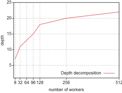
Depth of the decomposition Figure 1 shows the evolution of the depth depending on the number of workers. As expected, the depth of the decomposition grows with the number of workers. Sometimes, the depth is very high for some instances like ghoulomb 3-7-20 or talent scheduling alt film117 (see table 3). The reason is that the depth estimation we made is based on the Cartesian product of the domains which is sometimes wrong because there are many subproblems that are not consistent with the propagation, so the decomposition goes to a higher depth than the number of considered domains to generate 30 subproblems per worker consistent with the propagation.
Fig. 1. Depth to reach 30 subproblems per worker related to the number of workers.
Sequential decomposition issue Table 1 gives the part of the sequential decomposi-tion according to the overall resoludecomposi-tion time with 16 workers and 512 workers. For 16 workers, the sequential decomposition takes a small part of the overall resolution time (an average of 3.5%) because it generates few subproblems (16 ∗ 30 = 480 subprob-lems). Since the number of subproblems to generate is greater with 512 workers than 16 workers (16*30 vs 512*30), the sequential decomposition takes a significant time compared to the overall resolution time (an average of 72.5%). Thus, it takes more time to generate and impacts on the global performances.
Table 1. Part of the sequential decomposition according to the overall resolution time to generate 30 subproblems per worker for 16 workers and 512 workers.
Instance partdecf or 16 workers partdecf or 512 workers
16 ∗ 30 = 480 subproblems 512 ∗ 30 = 15360 subproblems
% %
market split s5-02 0.7% 33.5%
market split u5-09 0.6% 29.4%
market split s5-06 0.6% 37.6% prop stress 0600 4.7% 81.0% nmseq 400 4.0% 85.3% prop stress 0500 3.5% 81.7% fillomino 18 6.2% 88.7% steiner-triples 09 3.1% 70.5% nmseq 300 8.1% 91.2% golombruler 13 1.7% 78.0% cc base mzn rnd test.11 6.1% 83.4% ghoulomb 3-7-20 6.9% 91.3%
pattern set mining k1 yeast 4.9% 83.6%
still life free 8x8 8.8% 90.6%
bacp-6 2.8% 69.7%
depot placement st70 6 3.8% 79.5%
open stacks 01 wbp 20 20 1 7.1% 86.7%
bacp-27 3.8% 76.5%
still life still life 9 6.0% 88.5%
talent scheduling alt film117 5.3% 91.1%
geometric average(%) 3.5% 72.5%
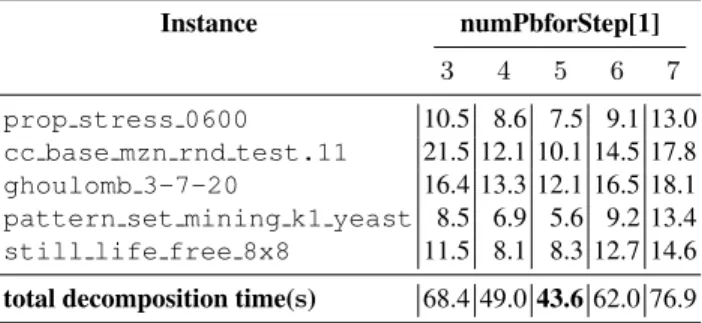
Fixing the parallel decomposition parameters Now, we must choose the number of subproblems to generate for the main phase. We select some representative instances to fix a good number of subproblems per worker. Table 2 shows the total decomposition time for some instance to choose the number of subproblems for the main phase. We no-tice that 5 is a good choice. Starting from 7 subproblems per worker, the performances begin to drop.
Table 2. Decomposition time comparison (in seconds) depending on the fixed number of sub-problems in the second phase with 512 workers.
Instance numPbforStep[1] 3 4 5 6 7 prop stress 0600 10.5 8.6 7.5 9.1 13.0 cc base mzn rnd test.11 21.5 12.1 10.1 14.5 17.8 ghoulomb 3-7-20 16.4 13.3 12.1 16.5 18.1 pattern set mining k1 yeast 8.5 6.9 5.6 9.2 13.4 still life free 8x8 11.5 8.1 8.3 12.7 14.6 total decomposition time(s) 68.4 49.0 43.6 62.0 76.9
Table 3. Comparison of the decomposition algorithms with 512 workers. Instance Seq. Decseq Dec//1 Dec//2
t0 sures tdec su tdec su tdec su
s r s r s r s r market split s5-02 3314.4 459.5 3.6 305.5 1.3 388.7 1.0 405.9 market split u5-09 3266.6 455.0 3.0 321.2 1.1 394.7 0.8 411.8 market split s5-06 3183.9 436.0 4.4 272.0 2.2 334.8 1.0 384.0 prop stress 0600 2729.2 213.9 54.4 40.7 21.3 80.0 7.5 193.1 nmseq 400 2505.8 429.7 33.7 63.3 14.9 120.9 4.6 240.4 prop stress 0500 1350.6 265.2 22.7 48.6 9.3 93.7 3.3 161.6 fillomino 18 763.9 301.9 19.8 34.2 6.4 85.7 2.5 150.7 steiner-triples 09 604.9 443.8 3.3 130.8 1.8 191.5 0.5 332.0 nmseq 300 555.3 309.0 18.7 27.1 7.9 57.1 2.4 131.7 golombruler 13 1303.9 492.0 9.4 92.7 1.4 322.9 0.4 427.9 cc base mzn rnd test.11 3279.5 196.5 83.8 32.6 35.5 62.8 10.1 122.6 ghoulomb 3-7-20 2993.8 279.2 112.6 24.3 50.0 49.3 12.1 131.1 pattern set mining k1 yeast 2871.3 285.5 51.3 46.8 21.0 92.4 5.6 183.2 still life free 8x8 2808.9 331.0 82.0 31.1 33.2 67.4 8.3 166.9 bacp-6 2763.3 473.1 13.4 143.5 5.4 245.0 1.5 378.9 depot placement st70 6 2665.1 345.6 29.9 70.9 12.5 131.8 3.6 235.1 open stacks 01 wbp 20 20 1 1523.2 280.7 35.4 37.3 15.6 72.3 4.0 160.8 bacp-27 1499.7 445.3 11.0 104.5 4.4 193.8 1.2 326.5 still life still life 9 1145.1 347.9 25.2 40.1 9.4 90.4 3.0 182.9 talent scheduling alt film117 566.1 386.4 15.0 34.4 6.0 75.8 1.8 175.8 total(s) and geom. average(r) 41694.5 347.1 632.6 66.4 260.8 124.8 75.0 223.9
Comparison of the decomposition algorithms We denote Decseq, Dec//1and Dec//2
respectively the sequential decomposition, the naive parallel decomposition and the new parallel decomposition.
Table 3 compares the decomposition time between different decomposition meth-ods with 512 workers and the speedup su of each decomposition algorithm. On the first hand, we observe that the average speedup of the resolution time without the decompo-sition time is closed to a linear factor (347.1). On the other hand, we notice that Dec//1
improves Decseqby a factor of 3.4 and Dec//2improves Dec//1by a factor of 2.4. So,
the new parallel decomposition method improves the decomposition. Consequently, the new parallel decomposition Dec//2 improves the overall speedup su from 66.4 with
the sequential decomposition Decseqto 223.9.
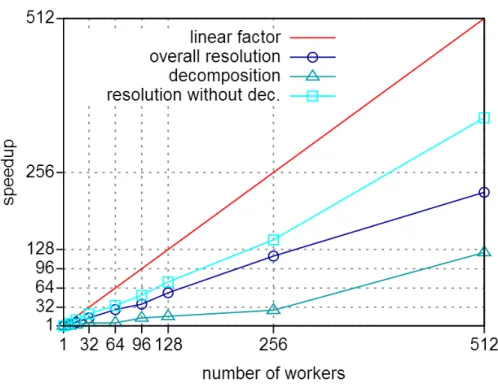
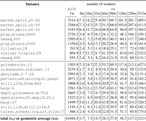
Scaling analysis We test the scalability of EPS for different numbers of workers. Table 4 describes the details of the speedups. We notice that the resolution of Golomb-ruler and the market-split instances scales very well with EPS (speedups su reach around 400 for 512 workers). Instances cc base mzn rnd test.11 and ghoulomb 3-7-20 give the worst results with all workers. In general, we observe an average speedup near to w/2. Figure 2 describes the speedup obtained by EPS for the decomposition phase,
the resolution phase without taking account the decomposition phase and the overall resolution with all instances (by a geometric average) as a function of the number of workers. EPS scales very well with a near-linear factor of gain for the resolution phase. Thanks to the parallelization of decomposition, EPS obtains good results for the overall resolution.
Table 4. Speedup detailed for each instance and for each number of workers with EPS. Instance number of workers
t0(s) su
1w 8w 16w 32w 64w 96w 128w 256w 512w market split s5-02 3314.4 7.3 14.2 25.4 50.7 69.7 101.5 201.7 405.9 market split u5-09 3266.6 7.3 14.3 25.7 51.5 68.6 103.0 207.4 411.8 market split s5-06 3183.9 6.4 12.7 24.0 48.0 64.0 96.0 197.5 384.0 prop stress 0600 2729.2 3.8 6.7 16.1 24.1 32.2 48.3 104.2 193.1 nmseq 400 2505.8 4.1 7.2 15.0 30.1 40.1 60.1 117.7 240.4 prop stress 0500 1350.6 2.5 4.4 13.1 20.2 26.9 40.4 81.8 161.6 fillomino 18 763.9 2.4 5.1 11.4 18.8 25.1 37.7 72.4 150.7 steiner-triples 09 604.9 5.7 12.3 21.7 41.5 55.3 83.0 143.2 332.0 nmseq 300 555.3 2.4 5.1 8.2 16.5 21.9 32.9 69.3 131.7 golombruler 13 1303.9 7.3 14.7 27.3 53.7 89.5 117.4 213.1 427.9 cc base mzn rnd test.11 3279.5 1.7 5.1 8.9 14.3 20.4 30.6 59.7 122.6 ghoulomb 3-7-20 2993.8 2.3 3.9 8.2 17.4 21.8 32.8 76.3 131.1 pattern set mining k1 yeast 2871.3 2.9 5.8 11.5 23.9 30.5 45.8 91.6 183.2 still life free 8x8 2808.9 2.6 6.4 10.4 20.9 27.8 41.7 83.5 166.9 bacp-6 2763.3 6.7 12.1 23.7 47.4 63.1 94.7 212.4 378.9 depot placement st70 6 2665.1 3.4 7.3 14.7 29.4 39.2 58.8 147.6 235.1 open stacks 01 wbp 20 20 1 1523.2 3.1 6.5 10.0 23.1 26.8 40.2 95.4 160.8 bacp-27 1499.7 5.6 11.2 20.4 43.8 54.4 81.6 214.3 326.5 still life still life 9 1145.1 3.1 6.1 11.4 22.9 30.5 45.7 89.4 182.9 talent scheduling alt film117 566.1 2.4 4.3 11.0 22.0 31.3 51.7 95.9 175.8 total (t0) or geometric average (su) 41694.5 3.7 7.5 14.7 28.3 37.9 56.7 117.3 223.9
Table 5. Comparison between work stealing and EPS with 512 workers. Instance Seq. Work stealing EPS
time(s) time(s) su time(s) su market split s5-02 3314.4 - - 8.2 405.9 market split u5-09 3266.6 - - 7.9 411.8 market split s5-06 3183.9 - - 8.3 384.0 prop stress 0600 2729.2 1426.4 1.9 14.1 193.1 nmseq 400 2505.8 - - 10.4 240.4 prop stress 0500 1350.6 670.0 2.0 8.4 161.6 fillomino 18 763.9 - - 5.1 150.7 steiner-triples 09 604.9 79.0 7.7 1.8 332.0 nmseq 300 555.3 - - 4.2 131.7 golombruler 13 1303.9 15.5 83.9 3.0 427.9 cc base mzn rnd test.11 3279.5 - - 26.8 122.6 ghoulomb 3-7-20 2993.8 575.4 5.2 22.8 131.1 pattern set mining k1 yeast 2871.3 299.8 9.6 15.7 183.2 still life free 8x8 2808.9 1672.8 1.7 16.8 166.9 bacp-6 2763.3 330.1 8.4 7.3 378.9 depot placement st70 6 2665.1 1902.9 1.4 11.3 235.1 open stacks 01 wbp 20 20 1 1523.2 153.9 9.9 9.5 160.8 bacp-27 1499.7 579.6 2.6 4.6 326.5 still life still life 9 1145.1 140.1 8.2 6.3 182.9 talent scheduling alt film117 566.1 95.5 5.9 3.2 175.8 total (time) or geometric average (su) 41694.5 7941 5.4 195.7 223.9
5.2 Comparison with work stealing
Table 5 shows a comparison between EPS and a work stealing implementation with 512 workers. The work stealing used in the datacenter is an MPI implementation based on [10]. In our experiments, the work stealing obtains good speedup until 64 workers but for more workers, the performances drop dramatically. With 512 workers, the aver-age speedup of work stealing is 5.4. Many instances are not solved with 512 workers whereas they are solved by the sequential resolution. However, the average speedup of EPS is 223.9. Note that EPS is better than the work stealing on all selected instances.
6
Conclusion
The previous decomposition algorithms of the Embarrassingly Parallel Search are ac-ceptable methods when there is only a few number of workers. These methods limit the performance of EPS on a data center, that is on a system with hundreds of cores. In this paper, we described an efficient parallel version of the decomposition. With paralleliz-ing the problem decomposition and fixparalleliz-ing 2 phases durparalleliz-ing the process, EPS gets a better workload during the decomposition. Consequently, EPS reaches the scalability with a data center and gives an average speedup at 223.9 with gecode for a set of benchmarks on a machine with 512 cores. This clearly improves the work stealing approach which does not scale well with hundred cores. EPS is more efficient by one or two orders of magnitude.
References
1. Gecode 4.0.0. http://www.gecode.org/, 2012.
2. F. Warren Burton and M. Ronan Sleep. Executing functional programs on a virtual tree of processors. In Proceedings of the 1981 Conference on Functional Programming Languages and Computer Architecture, FPCA ’81, pages 187–194, New York, NY, USA, 1981. ACM. 3. Geoffrey Chu, Christian Schulte, and Peter J. Stuckey. Confidence-Based Work Stealing in
Parallel Constraint Programming. In Ian P. Gent, editor, CP, volume 5732 of Lecture Notes in Computer Science, pages 226–241. Springer, 2009.
4. Robert H. Halstead, Jr. Implementation of multilisp: Lisp on a multiprocessor. In Proceed-ings of the 1984 ACM Symposium on LISP and Functional Programming, LFP ’84, pages 9–17, New York, NY, USA, 1984. ACM.
5. Joxan Jaffar, Andrew E. Santosa, Roland H. C. Yap, and Kenny Qili Zhu. Scalable Dis-tributed Depth-First Search with Greedy Work Stealing. In ICTAI, pages 98–103. IEEE Computer Society, 2004.
6. H˚akan Kjellerstrand. http://www.hakank.org/, 2014.
7. Tarek Menouer, Bertrand Cun, and Pascal Vander-Swalmen. Partitioning methods to paral-lelize constraint programming solver using the parallel framework bobpp. In Ngoc Thanh Nguyen, Tien Do, and Hoai An Thi, editors, Advanced Computational Methods for Knowl-edge Engineering, volume 479 of Studies in Computational Intelligence, pages 117–127. Springer International Publishing, 2013.
8. Laurent Michel, Andrew See, and Pascal Van Hentenryck. Transparent Parallelization of Constraint Programming. INFORMS Journal on Computing, 21(3):363–382, 2009. 9. MiniZinc. http://www.g12.csse.unimelb.edu.au/minizinc/, 2012.
10. Morten Nielsen. Parallel search in gecode. PhD thesis, Masters thesis, KTH Royal Institute of Technology, 2006.
11. Vasco Pedro and Salvador Abreu. Distributed Work Stealing for Constraint Solving. CoRR, abs/1009.3800:1–18, 2010.
12. Laurent Perron. Search Procedures and Parallelism in Constraint Programming. In Joxan Jaf-far, editor, CP, volume 1713 of Lecture Notes in Computer Science, pages 346–360. Springer, 1999.
13. Jean-Charles R´egin, Mohamed Rezgui, and Arnaud Malapert. Embarrassingly parallel search. In Christian Schulte, editor, Principles and Practice of Constraint Programming, volume 8124, pages 596–610. Springer Berlin Heidelberg, 2013.
14. Christian Schulte. Parallel Search Made Simple. In ”Proceedings of TRICS: Techniques foR Implementing Constraint programming Systems, a post-conference workshop of CP 2000, pages 41–57, Singapore, 2000.
15. Feng Xie and Andrew J. Davenport. Massively Parallel Constraint Programming for Su-percomputers: Challenges and Initial Results. In Andrea Lodi, Michela Milano, and Paolo Toth, editors, CPAIOR, volume 6140 of Lecture Notes in Computer Science, pages 334–338. Springer, 2010.
16. Peter Zoeteweij and Farhad Arbab. A Component-Based Parallel Constraint Solver. In Rocco De Nicola, Gian Luigi Ferrari, and Greg Meredith, editors, COORDINATION, volume 2949 of Lecture Notes in Computer Science, pages 307–322. Springer, 2004.