HAL Id: halshs-01093414
https://halshs.archives-ouvertes.fr/halshs-01093414
Submitted on 10 Dec 2014
HAL is a multi-disciplinary open access
archive for the deposit and dissemination of sci-entific research documents, whether they are pub-lished or not. The documents may come from teaching and research institutions in France or abroad, or from public or private research centers.
L’archive ouverte pluridisciplinaire HAL, est destinée au dépôt et à la diffusion de documents scientifiques de niveau recherche, publiés ou non, émanant des établissements d’enseignement et de recherche français ou étrangers, des laboratoires publics ou privés.
Resuming bank lending in the aftermath of the Capital
Purchase Program
Varvara Isyuk
To cite this version:
Varvara Isyuk. Resuming bank lending in the aftermath of the Capital Purchase Program. 2014. �halshs-01093414�
Documents de Travail du
Centre d’Economie de la Sorbonne
Resuming bank lending in the aftermath of the Capital Purchase Program
Varvara ISYUK
Resuming bank lending in the aftermath of the Capital
Purchase Program
Varvara Isyuk
∗July 2014
Abstract
In the second half of 2008, after a series of bankruptcies of large financial institu-tions, the U.S. Treasury poured capital infusions into domestic financial institutions under the Capital Purchase Program (CPP), thus helping to avert a complete collapse of the U.S. banking sector. In this article the effectiveness of the Capital Purchase Program is analysed in terms of restoring banks’ loan provisions. The relative impacts of liquidity shortages (which negatively affected banks’ willingness to lend) and the contraction in aggregate demand for bank loans are examined. The empirical evidence on the effects of capital shortages supports the theory. Banks that have a higher level of capitalisation tend to lend more both during the crisis and in normal times. More-over, it is found that bailed-out banks displayed higher growth rates of loans during the crisis than in normal times (before 2008) as well as higher rates compared with non-bailed banks during the crisis, with a one percentage point increase in the cap-ital ratio. In addition, bailed-out banks that repurchased their shares from the U.S. Treasury provided more loans during the crisis than those banks that did not.
Keywords: Capital Purchase Program, bank lending, credit growth, liquidity provisions
JEL Classification Numbers: E58, G21, G28
∗CES Centre d’Economie de la Sorbonne, Universit´e Paris 1 Panth´eon Sorbonne, National Bank of
R´esum´e
Dans la seconde moiti´e de 2008, apr`es une s´erie de faillites de grandes institutions financi`eres, la R´eserve F´ed´erale am´ericaine a r´eagi au manque de liquidit´e `a travers la garantie obligatoire des prˆets et des recapitalisations bancaires principalement dans le cadre du Capital Purchase Program (CPP) pour les banques commerciales pour afin ´eviter l’effondrement du secteur bancaire am´ericain. Dans cet article l’efficacit´e du CPP est analys´ee en termes de restauration d’octroi de cr´edits bancaires. Les impacts relatifs du manque de liquidit´e (qui a n´egativement affect´e la volont´e des banques `a prˆeter) et de la baisse de la demande globale pour les prˆets bancaires sont examin´es. La preuve empirique sur les effets du manque de liquidit´e soutient la th´eorie. Les banques avec un niveau de capitalisation ´elev´e ont tendance `a octroyer plus de cr´edits au cours de la crise et en temps normal. En outre, les banques renflou´ees ont affich´e des taux de croissance des prˆets plus ´elev´es au cours de la crise qu’en temps normal (avant 2008) ainsi que des taux plus ´elev´es par rapport aux banques non-renflou´ees pendant la crise, avec une augmentation d’un point de pourcentage du ratio de capital. De plus, les banques renflou´ees qui ont rachet´e leurs actions aupr`es du Tr´esor am´ericain offraient plus de prˆets au cours de la crise que les banques qui ne l’ont pas fait.
1
Introduction
The well-functioning banking sector is often said to play a crucial role in cultivating business activity. Indeed, financial distress as well as the lack of confidence that undermined banking activity during the crisis of 2007 immediately affected the real economy. Govern-ments had to undertake conventional and ad hoc measures offering liquidity in the form of bailout packages. The main program that provided liquidity to U.S. commercial banks was the Capital Purchase Program (CPP). The goal of these interventions was to stabilise the financial system by providing capital to viable financial institutions (see details in Isyuk, 2013a). However, there is still no clear evidence of the efficacy of public (as opposed to market-based) capital injections for sustaining bank loan growth.
Empirical studies show that loan provisions to the private sector tend to slow down during banking crises (Kaminsky and Reinhart, 1999; Eichengreen and Rose, 1998; Demirg¨u¸c-Kunt et al., 2006). There can be several reasons for that. On one hand, the literature focuses on the vulnerability of banks’ balance sheets and their sensitivity to liquidity shortage. That transmission channel of credit supply to the real economy is investigated in Black and Rosen (2009); Hirakata et al. (2009); De Haas and van Horen (2010); Berrospide and Edge (2010); Brei et al. (2011). It is confirmed that the bank’s balance sheets position greatly affects the bank’s credit offer to enterprises and individuals.
On the other hand, credit growth can decelerate not only due to the financial conditions of the bank and its willingness to lend, but also due to the deterioration in demand for bank products and services. The same adverse exogenous shocks that triggered the problems with bank’s liquidity can induce the decline in the aggregate demand (Dell’Ariccia et al., 2008). The overall decline in economic activity negatively affects the willingness of the individuals and firms to borrow, both for consumption and investments. Besides, as highlighted in Dell’Ariccia et al. (2008), the credit cycle effect `a la Kiyotaki and Moore (Kiyotaki and Moore, 1997) can occur during the crisis. In that case, even creditworthy borrowers see the value of their collaterised assets (as well as their balance sheets) to deteriorate, which leads to a decline in the credit offer, even by healthy banks.
Thus, there is a link with the literature focusing on disentangling the relative impacts of demand and financial shocks (Tong and Wei, 2009b; Claessens et al., 2012). These authors suggest several indexes for measuring the sensitivity of the nonfinancial firms to demand shocks that could be also applied to the financial sector.
This paper uses the methodology of Brei et al. (2011) in order to estimate the impact of bank capital, other bank balance sheet characteristics, and sensitivity to demand shocks on bank lending. That framework allows for the introduction of structural changes in parameter
estimates for the period of the crisis and for normal times, as well as for bailed-out and non-bailed banks. While Brei et al. (2011) focus on the data regarding 108 large international banks, in this paper the focus is on the U.S. commercial banks and the role of the CPP in resuming bank lending.
This paper contributes to the literature on the efficacy of public capital injections during the crisis. It provides the framework in which the sensitivity of the bank’s credit offer to financial distortions and its sensitivity to decline in aggregate demand are separated from each other1. The relationship between bank balance sheet characteristics, sensitivity to the
demand shock, and bank credit growth is analysed for the banks that received CPP funds and the banks that did not participate in the CPP in normal times and during the crisis. Moreover, the same relationship is also investigated for the subsample of the financial firms that received the CPP funds in order to distinguish between the banks that repurchased their stake from the U.S. Treasury and the banks that did not repurchase their stake by July of 2012.
The great deal of this paper is focused on pre-testing the models and selecting the ad-equate instruments for the estimators with instrumental variables. The full version of this paper (Chapter 4, Isyuk, 2013b) includes six types of estimators that prove to be to some extent more and to another extent less advantageous when dealing with particular economet-ric issues. The detailed results are presented only for Mundlak-Krishnakumar and Blundell-Bond system GMM models, while the summary results for all estimators are presented in section 4.3. I start with fixed effects estimator that, however, does not allow us to obtain the parameter estimates for the time-invariant variables (such as bailout or repayment dummy). Besides, as the model is dynamic, the fixed effects estimator is inefficient and might lead to inconsistent estimates. The Mundlak-Krishnakumar model (Mundlak, 1978; Krishnakumar, 2006) is then conducted and, on one hand, provides the estimates for time-invariant variables and, on the other hand, following Chatelain and Ralf (2010), is used as a pre-test estimator that helps to select instrumental variables for further estimations. The Hausman-Taylor estimator (Hausman and Taylor, 1981) enables the separation between exogenous and en-dogenous time-variant and time-invariant variables. With regard to the enen-dogenous nature of the bailout dummy, it is expected to obtain consistent and efficient estimates using that method.
The logit regression from Isyuk, 2013a is then used as a first-stage in the Two Stage Least Squares (2SLS) model based on instrumental variables (IV). The bailout dummy is
1
In most of empirical studies, demand factor is proxied by changes in the GDP of the country. It means that they do not take into account heterogenous reactions of the financial institutions to the changes in aggregate demand (see Berrospide and Edge, 2010; Brei et al., 2011).
instrumented using the proxy for systemic risk (beta) and the share of mortgage-backed securities in a bank’s total assets. The fitted values of bailout dummy are then plugged into the second stage regression. The final models are Arellano-Bond first-difference (Arellano and Bond, 1991) and Blundell-Bond estimators (Blundell and Bond, 1998) that use Gener-alised Method of Moments-style (GMM) instruments and are often referred to as one of the most efficient estimators when working with large number of observations and small-time dimension datasets and when fitting the dynamic model.
The empirical evidence on the effects of capital shortage supports the theory. Banks with a higher level of capitalisation tend to lend more both during the crisis and in normal times. This result is in line with that of Francis and Osborne (2009), who use data on U.K. banks and report that better-capitalised banks are more willing to supply loans. The same is confirmed by Foglia et al. (2010), who also find that this effect is intensified during the crisis.
Moreover, during the crisis, bailed-out banks exhibited higher growth rate of loans than in normal times (before 2008) and higher than that of non-bailed banks during the crisis, with a one percentage point increase in capital ratio. This means that liquidity provisions to the banks during the recent crisis supported bank lending. Besides, these results extend those from Isyuk (2013a) suggesting that bailed-out banks were also the ones that could contribute to a larger extent to the rise in credit offer. It also seems that the banks that were characterised as specialised in commercial and industrial lending and that exhibited higher probability of receiving CPP funds (see Isyuk, 2013a for details) were also the ones that contributed to a larger extent to the growth rates of loans (thus, mostly commercial and industrial loans, as they were specialised in that type of lending).
The same results also show that during the crisis, more capital is required for the non-bailed banks to sustain the growth of credit supply on a pre-crisis level. In tough times, additional capital is not that easily translated into extended credit offers by the banks that did not benefit from the CPP program, as they prefer to keep a substantial part of it for their internal needs.
It seems that the banks that repaid CPP funds by July 2012 were the ones that received enough additional capital to support their operations during the crisis and to continue provid-ing credits to enterprises and individuals. In their case, the recapitalisation scheme worked efficiently, providing them the possibility to repurchase their stake from the Treasury and to translate additional capital into more lending.
It is also in line with the results of Brei et al. (2011), who argue that the banks-recipients of CPP funds start to translate additional capital into greater lending during the crisis once their capitalisation exceeds a critical threshold. That critical threshold should also
account for the commitment to reimburse the CPP funds. The bank that is not capable of repurchasing its stake from the Treasury cannot be expected to expand the credit offer to enterprises and individuals. It is more probable that such a bank will adjust its assets portfolio to meet the capital requirements by cutting the number of newly issued loans.
The rise in aggregate demand contributes to the increase in bank lending in good times. However, during the crisis, the situation changes, especially for different types of loans. For instance, since 2007, the demand factor has had no impact on the growth rates of real estate mortgage loans for non-bailed banks. With the collapse in housing markets and generally unstable economic situation, consumers were less willing to take new mortgages.
The rest of the paper is structured as follows. Section 2 presents the description of the model, estimators, econometric issues related to endogeneity bias as well as the selection procedure of the optimal instruments for system GMM. The data and the construction of variables are explained in section 3. Section 4 reviews the detailed results for Mundlak-Krishnakumar and Blundell-Bond system GMM models as well as summarizes the results from other estimators in section 4.3. Section 5 concludes.
2
Model and estimation methodology
2.1
Model
In this empirical model, bank lending between 1995 and 2011 is explained by two core factors: banks’ financial constraint (or, in other words, the level of capitalisation) and their sensitivity to the shocks on aggregate demand. However, the period between 1995 and 2011 includes intensive growth (2001-2006), recession (2007-2009), as well as the period of sluggish economic growth following the recession (after 2009). Besides, substantial liquidity injections into the banking sector under the CPP took place during the recession in 2008-2009.
Such particular conditions during the analysed period cannot be ignored. They represent significant structural changes that may have affected the relationship between bank-specific factors and bank lending.
Thus, the parameter estimates are allowed to change for two states of economy: crisis and normal times. Besides, the parameters shift for the banks-beneficiaries of the CPP funds relative to the banks that did not receive the funds. Moreover, the subsample of the banks-recipients of CPP funds is analysed in order to check for differences in the same relationship among the banks that repurchased their stock from the U.S. Treasury in short notice (before July 2012) and the ones that did not.
model via dummies and their interactions with individual financial bank characteristics and sensitivities to changes in aggregate demand.
The first full specification of the dynamic panel regression following Brei et al. (2011) and Gambacorta and Marques-Ibanez (2011) is the following:
∆Ln(Lit) = φ0+ φ1Ct+ η∆Ln(Li,t−1) + χ1Zt−1+ [χ + χ∗Ct] Bi
+ [δ + δ∗C
t+ (ω + ω∗Ct)Bi] BSCi,t−1+ αi+ ǫit (1)
where
• ∆Ln(Lit) is the growth rate of lending at the bank i during the year t ;
• BSCi,t−1are lagged bank-specific characteristics associated with financial and demand constraints of commercial bank i ;
• Zt−1 are lagged macroeconomic controls (real GDP growth, change in Federal Funds interest rate);
• Ct is the dummy that distinguishes between the crisis period and normal times;
• Bi indicates the banks that received the CPP funds relative to those that did not;
• αi represents random bank effects; and
• ǫit are observation-specific errors.
This model is estimated using fixed effects, Mundlak-Krushnakumar, Hausman-Taylor, Instrumental Variables (IV), Arellano-Bond first difference, and Blundell-Bond system GMM estimators. Each of these estimators transforms Equation 1 in a particular way in order to obtain efficient and consistent estimators. Clearly the estimators that are based only on within-transformation of the variables do not allow for the estimation of time-invariant variables, such as the bailout dummy. Hence, when using fixed effects and Arellano-Bond first difference estimators, the bailout dummy as well as the interactions between bank-specific variables and the bailout dummy are omitted from model 1, described above.
Another group of regressions is run on a subsample of 252 banks-recipients of CPP funds. The cofficients similar to those from the previous regression are marked herein with a subscript b. Here the differential relationship is allowed for the banks that redeemed their stake from the Treasury and those that did not:
∆Ln(Lit) = φb0+ φb1Ct+ ηb∆Ln(Li,t−1) + χbZt−1+ [χb+ χ∗bCt] Ri
+ [γ + γ∗C
t+ (κ + κ∗Ct)Ri] BSCi,t−1+ αbi+ ǫbit (2)
where Ri specifies the banks that reimbursed the CPP funds before July 2012 and the banks
that did not pay anything (in the subsample of banks-recipients of CPP funds).
The same estimators as for model 1 are used to estimate model 2. Ri is the time-invariant
repayment dummy, and thus, it is also omitted when using fixed effects and the Arellano-Bond first difference estimator.
Individual bank-specific characteristics BSCi,t−1 include balance sheet indicators that
account for supply factors that influence a bank’s decision regarding the offer of the loans. The bank’s financial constraint is mainly associated with its level of capitalisation. During the crisis, for instance, a bank’s capital ratio is expected to worsen due to the bank’s losses in subprime mortgage-related assets (it can also be any other adverse capital shock or even change in banking regulation). If the bank does not have enough capital buffer and cannot raise equity2, it is expected that the bank will tend to adjust its capital ratio by cutting the
number of newly issued loans.
In the literature, this question is often referred to as a trade-off between the marginal costs of issuing equity and the marginal cost of cutting back on lending. The results of the study conducted by Kiley and Sim (2010) suggest that the banks respond to a capital shock through a mix of financial disintermediation and recapitalisation. Besides, instead of just including macroeconomic controls on the country level (as was done, for instance, in Brei et al., 2011), the individual levels of sensitivity to changes in U.S. real GDP are computed. They account for heterogeneous reactions of commercial banks to expansion or contraction of the aggregate demand. These bank-specific sensitivities to changes in GDP are introduced as proxies for the impact of demand factors on the bank’s lending activity.
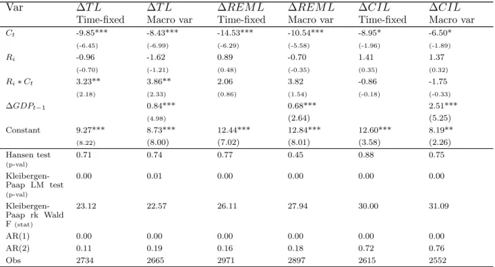
The basic idea of parameter estimates for interactions between crisis, bailout, and repay-ment dummies with sensitivity to GDP growth and balance sheet characteristics is similar. The estimation of the models described above results in the set of coefficients for any bank-specific factor (both balance sheet characteristic or sensitivity to demand shock), presented in table 1.
These various coefficients allow us to explore the impact of supply and demand factors on loan growth and to see how it changes (i) in the period of crisis compared to normal times; (ii) between the banks that received CPP funds and the banks that did not participate in
2
Table 1: Resulting set of coefficients for the bank-specific characteristic BSC1 and its
inter-actions with dummies from models 1 and 2
Banks/Periods No Crisis Crisis All banks
No Bailout δ1 δ1+ δ1∗
Bailout δ1+ ω1 δ1+ δ1∗+ ω1+ ω1∗
No Repayment γ1 γ1+ γ1∗
Repayment γ1+ κ1 γ1+ γ1∗+ κ1+ κ∗1
the CPP; and (iii) between the banks that repurchased their stake from the Treasury by July 2012 and the banks that did not. The fact of the bank bailout means that the bank applied for CPP funds, was approved by the U.S. Treasury and accepted the final conditions by providing required documentation. Conversely, there are two possible reasons that the bank did not to receive the bailout: either the bank did not apply for CPP funds (because it had access to alternative sources of financing or did not require recapitalisation during the crisis), or the bank’s application for participation in the CPP was rejected by the Treasury (for more discussion on that topic, see Isyuk, 2013a).
The coefficient δ1 shows the short-term impact of the change in variable BSC1 on bank
lending at non-bailed banks in normal times (Bi = 0; Ct = 0). The long-term effect is given
by δ1
1−η for model 1 or by δ1
1−ηb for model 2. When the coefficient δ
∗
1 is significant, it means
that the relationship between the underlined variable BSC1 and bank lending is significantly
different in crisis time compared to normal times for non-bailed banks. The full impact is then calculated as δ + δ∗. Other coefficients are interpreted in a similar way.
In tables with results individual coefficients δ, δ∗, ω, and ω∗ for model 1 and γ, γ∗, κ,
and κ∗ for model 2 are reported with stars identifying their level of significance, while the
coefficients measuring the full impact (δ + δ∗, δ + ω etc.) can be found in square brackets.
2.2
Endogeneity bias
Dynamic panel models 1 and 2 presented in section 2.1 allow for, on one hand, empirical modeling of dynamic effect through the lagged dependent variable (past behaviour affect-ing current one); on the other hand, individual-specific dynamics. When estimataffect-ing these models, however, several econometric issues related to endogeneity bias may arise. They are described below followed by the proposed solution in form of the alternative estimator.
ǫit. Nickell (1981) reports that standard methods of estimation such as within estimator
and Ordinary Least Squares (OLS) can lead to seriously biased coefficients in dynamic models (often referred to as ”fixed effects Nickell’s bias”). This issue is particularly important in case of panel datasets with large number of individuals and small number of time periods. It is said that within autoregressive parameter bias is larger when the number of time periods T is small (less than 10), negligible when T is larger than or equal to 30. In the full sample of banks examined in this paper the average number of available time periods is 10.1, while the maximum number of periods is 16 (annual data between 1995 and 2011), suggesting that the coefficients obtained via within estimator (presented in the following section) can be biased. The models that deal with autoregressive bias and that are designed for short time dimension and large entity dimension datasets are those based on Generalised Methods of Moments Estimator (GMM).
• Endogeneity of time-invariant variables Bi and Ri due to their correlation with
individual-level random effect. This issue can be treated using the Hausman-Taylor estimator (Hausman and Taylor, 1981). That estimator assumes that some of the ex-planatory variables are correlated with the individual-level random effects, but that none of the explanatory variables are correlated with the idiosyncratic error. Endoge-nous bias of time-invariant variables is corrected using internal instruments. In that sense Hausman-Taylor estimator improves over Fixed Effects (because it allows to es-timate the parameters for time-invariant variables) and over Mundlak-Krishnakumar estimator (that does not deal with the endogeneity of time-invariant variables).
• Endogeneity of time-varying indicators (such as bank-specific variables). That bias may arise due to correlation with individual random effects. Within transformation or first-differencing both permit to avoid that problem and obtain consistent parameter estimates.
• The presence of reverse causality. Loans growth rates are assumed to be endogenous; however, causality may run in both directions: bank-specific characteristics influence the growth rates of loans while the growth rates of loans affect bank-specific character-istics (for instance, capital ratio). Besides, the bailout dummy is endogenous as it is the consequence, on one hand, of the particular bank’s decision (as the bank chooses to apply or not for the Capital Purchase Program and later accepts or not the final conditions attached by the Treasury), on the other hand, of the Treasury’s decision (acceptance or refusal of the bank’s application for CPP funds, more on that see in
Isyuk, 2013a. In that case, the method of Instrumental Variables is efficient as it pro-vides unbiased coefficients for endogenous regressors through the two-step estimation procedure.
• Dealing with endogeneity bias using the instruments that are too many and weak. That is the issue that often arises when applying Arellano-Bond (Arellano and Bover, 1995) and system GMM (Blundell and Bond, 1998) estimators (see section 2.5). The proper instruments have to satisfy the conditions of validity (exogeneity) and relevancy that is not always the case. GMM estimators are supposed to deal with most of the endogeneity issues presented above, however, the consistency of the parameters obtained for time-invariant variables is not investigated so far.
2.3
Mundlak-Krishnakumar estimator
One of the estimators that allows to gauge the effects of time-invariant variable (as op-posed to the estimators such as fixed effects that only use information on within variance of covariates, ignoring the between variance) is Mundlak estimator (Mundlak, 1978), later extended by Krishnakumar (2006). This estimator not only helps to estimate the impact of time-invariant variables but also, when used as a pre-test estimator, to decide which time-varying variables are endogenous and which are not(Chatelain and Ralf, 2010). This information will be then useful in Hausman-Taylor, IV and GMM estimators that require distinguishing between exogenous and endogenous variables and selecting appropriate in-struments.
The basic methodology of Mundlak-Krushnakumar estimator is presented below. The model 1 contains both time-series cross-section data and time-invariant variables and can be rewritten in the following simplified form:
yit = βxit−1+ γbi+ αi+ ǫit (3)
where yit is dependent variable; xit−1 are lagged time and individual varying explanatory
variables; bi are time-invariant explanatory variables (or dummies); αiare individual random
effects, and β and γ are coefficients to be estimated for time-varying and time-invariant variables, respectively. The error term ǫit is assumed to be uncorrelated with xit−1, bi and αi.
As there is no theoretical evidence yet on the adequacy of Mundlak model with autoregressive variables, lagged dependent variable yit−1 is removed from the model.
The difficulty of estimation of that model is the potential correlation of individual effects αi with xit−1 and especially with time-invariant variables bi. Mundlak (1978) proposes to
αi = πxi◦+ φbi+ αiM (4)
where xi0 is average over time for each individual of time-varying variables, π and φ are
coefficients to be estimated for these averages and time-invariant variables, respectively. Combining auxiliary regression with initial regression yields the following equation:
yit= βxit−1+ (γ + φ)bi+ πxi◦+ αMi + ǫit (5)
Applying Generalised Least Squares (GLS) model to estimate the last equation, Mundlak (1978) showed that [ βGLS = cβW (6) [ πGLS = cβB− cβW (7) [ γGLS =γcB (8)
where cβB and γcB are between estimators, while cβW is a within estimator3.
For each time-varying variable xi◦ Mundlak-Krishnakumar regression tests the null hy-pothesis cβB− cβW = 0 (Equation 7). Thus, the smaller and the closer to zero is the estimated
parameter π[GLS, the more exogenous variable xi◦ is. Later these exogenous xi0 variables
can be used as instruments in Hausman and Taylor (Hausman and Taylor, 1981) and other estimators (Chatelain and Ralf, 2010).
2.4
Two-step system GMM estimator
In this paper the system GMM is preferred to difference GMM as it allows to include time-invariant regressors into the model as well as to account for heteroscedasticity of model errors.
System GMM is the augmented version of the difference GMM estimator. Initially it was developed to improve the difference GMM estimators as lagged levels were often poor instruments for first-differenced variables4. Arellano and Bover (1995) and Blundell and
Bond (1998) modified the difference GMM estimator by adding the original level equation to the system. The instruments for the variables in levels are their own lagged first-differences.
3
Mundlak also proved them to be best linear unbiased estimators (BLUE).
4
The larger number of instruments allows to increase the efficiency of the estimator.
Two-step system GMM provides an algorithm for computing the feasible efficient two-step GMM estimator, where residuals from the first step are used to form the optimal weighting matrix. The efficient GMM estimator is then estimated using that matrix. Therefore the two-step GMM estimates are robust to the presence of heterescedasticity and serial correlation. The cost of the increased efficiency of system GMM estimator is a set of additional restrictions on initial conditions. Basically it requires first-differences to be uncorrelated with unobserved group effects. Another disadvantage of applying the system GMM estimator is an important rise in the instrument count. In case the lag range is not restricted and the instrument matrix is not collapsed, each instrumenting variable generates one column for each time period and each lag available in that time period. As highlighted in Roodman (2006), the number of instruments is then quadratic in T.
Often referred to as ”too many instruments” problem, it can lead to, first of all, over-fitting of endogenous variables which could bias coefficient estimates toward those from non-instrumenting estimators. Second, high instrument count could become the reason of imprecise estimates of the GMM optimal weighting matrix and, consequently, downward biased standard errors (see Roodman, 2008 for more details).
The bias and the standard errors can be lowered by using the Windmeijer correction (Windmeijer, 2005) for the two-step efficient GMM. The solution for the former problem requires keeping the number of instrument lags low. The choice of instruments and their lags is described in the next section following the strategies in the literature on the performance of the IV and GMM estimators (Chatelain and Teurlai, 2001; Donald et al., 2009; Mehrhoff, 2009). Additional tests on relevancy and validity of the instruments are presented in section 2.5.
2.5
Choice of instruments for system GMM
2.5.1 Limiting the number of moment conditions
If the number of instruments is too large, GMM estimator becomes inconsistent. In case the number of instruments is not constrained, each instrumenting variable generates one column for each time period and lag available in that time period (Roodman, 2006). In this section 23 variables are treated as endogenous or predetermined for full specifications of models 1 and 2:
• six main variables (lagged dependent variable and 5 bank specific characteristics (BSCit));
• interaction of five BSCit with crisis dummy;
• interaction of five BSCit with bailout (or repayment) dummy;
• interaction of five BSCit with both crisis and bailout (or repayment) dummies;
• bailout (or repayment) dummy and its interaction with crisis dummy (two in total).
The equation is said to be exactly identified when there are at least as many instruments generated as included endogenous variables. On the other hand, the optimal weighting ma-trix of the GMM estimator has a rank of N (number of banks) at most. This mama-trix becomes singular and the two-step estimator cannot be computed when the number of instruments exceeds N (Soto, 2009). As the sample contains information on almost 550 financial insti-tutions, the number of generated instruments in system GMM should not exceed 550.
In case the count of moment conditions is not reduced, the standard instrument set providesT(T −1)2 = 105 moment conditions for a single lagged dependent variable, (T −2)(T −1)2 = 91 moment conditions for each endogenous variable and T − 1 = 14 moment conditions for each exogenous variable (Mirestean and Charalambos, 2009).
To reduce the instrument count two main techniques are used:
• Limiting the lag length is based on the selection of the lags to be included in the instrument set. Baum et al. (2002) advises to constrain the lags between the second and the fifth. In that case the number of moment conditions will be equal to the number of instrumented variables (exogenous, endogenous or predetermined) multiplied by the number of lags used.
• Collapsing the instrument set also allows to make the instrument linear in T. The columns of the original instrument matrix are ”collapsed” reflecting the fact that orthogonality condition has to be valid for each lag but not any more for each time period.
Some additional transformations can be applied on the instrument set. For instance Mehrhoff (2009) proposes to apply the Principal Component Analysis (PCA) to the instru-ment set. The transformation matrix becomes then stochastic rather than deterministic. After performing Monte-Carlo simulations the author finds that factorised instruments pro-duce the lowest bias and standard errors, while recommends to collapse the matrix prior to factorisation.
2.5.2 Selection of the optimal instruments
It is not only the instrument count that influences the choice of the instruments for GMM estimations but also the ”quality” of these instruments. There exists two criterias for proper instrumental variables in linear IV and GMM regressions. The ”good” instruments have to be:
• correlated with endogenous regressors;
• orthogonal to the error process (or, in other words, exogenous);
In the literature the first condition is often referred to as the ”relevancy” of instruments, while the second one referred to as the ”validity” of instruments. Instruments are said to be weak and the system to be weakly identified, if the instruments are weakly correlated with endogenous regressors (Stock et al., 2002; Bun and Windmeijer, 2010).
There are several methods to deal with the problem of instrument relevance. In this article the correlation coefficients between the set of instruments and endogenous variables are first analysed for each equation. Thus, the correlation tables that report the correlation coefficients between lagged variables in levels (dependent and explanatory variables until the fourth lag) and differenced variables Yit−Yit−1, Yit−1−Yit−2, Xit−1−Xit−2 are constructed
for the first-difference equation. Accordingly such tables are constructed for the variables from the equation in levels but reporting the correlation between lagged first-differences and variables in levels Yit, Yit−1 and Xit−1 (see Appendix A).
The deeper lags of level variables (for the first difference equation) and those of first differences (for the level equation) have a larger probability of being weaker instruments, i.e. being weekly correlated with endogenous regressors5. However, the first lags of instruments
might be highly correlated with the dependent variable Yit and its first difference Yit−Yit−1
which may cast a doubt on the orthogonality between instruments and errors. As mentioned above, the deeper lags might be preferred to the lower ones because they provide a higher probability of instrument independence from unobserved error process. Thus, when selecting the instruments, the trade-off between the level of weakness of the instruments and their exogeneity is taken into account.
Besides, the corresponding moment conditions can be tested if the system of equations is overidentified6. It can be done via Hansen statistic in the presence of heteroscedasticity or via
Sargan statistic under the assumption of conditional homoscedasticity. Heteroscedasticity is detected in these regressions, so it is the Hansen statistic that is reported in the resulting
5
That is why the lags deeper than the fourth lag are not analysed.
6
tables. The null hypothesis of the test implies that the instruments satisfy the orthogonality conditions required for their employment (Baum et al., 2002), and that all together they are valid instruments.
In order to additionally check the orthogonality of some instruments or subset of instru-ments, the Difference-in-Sargan/Hansen statistic (or C-statistic) is analysed. That statistic basically measures the difference in Sargan/Hansen statistics computed, on one hand, for the regression with the full set of instruments, on the other hand, for the regression with a particular (tested) set of instruments removed from the full one. The null hypothesis is that of the valid subset of instruments.
The two-step robust regressions that normally produce asymptotically more efficient es-timators are conducted7. It makes the estimators consistent in the presence of any pattern
of heteroscedasticity or autocorrelation.
2.5.3 Testing for underidentification and weak instruments
Empirical tests of overdientifying restrictions are often criticized for having a low power. Besides, as highlighted by Bazzi and Clemens (2013), multiple instruments do not allow the detect the possibility of the most valid instruments to be the weakest and the strongest to be the the least valid.
Besides, the first stage regressions where endogenous variables are regressed on the full set of instruments are examined. The Bound et al. (1995) F-statistics and ”partial” R2 as well as
the Shea’s partial R2 (which is is more relevant as there is more than one endogenous regressor
in the model) are analysed for several instrument subsets in order to choose sufficiently relevant endogenous regressors.
The Bound et al. (1995) F-statistic allows us to measure the significance of a particular instrument by excluding this instrument from the regression. It is the ”squared partial correlation” between the excluded instrument or a subset of instruments and endogenous regressor that is in question, RSSI1−RSSI
T SS , where RSSI1 is the residual sum of squares in the
regression instrumented with I1, RSSI is the residual sum of squares in the regression with
the full set of instruments (see Baum et al., 2002 for more details).
However, it is not an efficient measure of the fit of regressions, if there are multiple endogenous regressors in the model. The intercollerations among the regressors need to be taken into account. The Shea’s partial R2 is a more consistent measure of the regression’s
fit in that case.
Thus, additional tests for identification and weak instruments are applied in the paper
7
A finite-sample Windmeijer correction to the two-step covariance matrix is applied to correct otherwise downward biased standard errors.
following Bazzi and Clemens (2013); Stock and Yogo (2002). The strength of identifica-tion is tested via the test of the rank of a matrix based on the Kleibergen-Paap (2006) rk statistic. The test allows to check whether the equation is identified, i.e., that the excluded instruments are correlated with the endogenous regressors. The null hypothesis of the test is that the equation is underidentified, meaning when partialling out exogenous covariates and other cross-correlations with endogenous variables and instruments, the weakest correla-tion between an instrument and one of the endogenous variables does not contribute enough variation to add a rank of the instrument matrix (Bazzi and Clemens, 2013). A rejection of the null indicates that the matrix is full column rank and, thus, that the model is identified. The p-values for the Kleibergen-Paap rk statistic under the assumption of heteroscedasticity are presented in tables.
Another group of statistics includes Cragg-Donald Wald and Kleibergen-Paap Wald statistics and allows to test for weak identification. In case of weak identification the corre-lation between endogenous regressors and excluded instruments is small. However, Cragg-Donald Wald statistic is only valid under the assumption of identically and independently distributed errors (i.i.d.). Thus, it is mostly the second one Kleibergen-Paap Wald F-statistic that is reported.
Following Stock and Yogo (2002), the definition of weak instruments in terms of the relative bias is adopted. A group of instruments is weak if the bias of the IV estimator, relative to the bias of ordinary least squares (OLS), exceeds a certain threshold (5%, 10% or 30% are reported). Relevant critical values for Kleibergen-Paap Wald F-statistic (thus, for the case with robust standard errors) have not been tabulated. However, it is advised in the literature (for instance, by Baum et al., 2007) to apply though with caution the Stock and Yogo critical values initially tabulated for Cragg-Donald statistic. Stock and Yogo critical values are not tabulated for cases with more than three endogenous variables. As in the regressions from this paper there are mostly more than three endogenous variables entering the regressions, the critical values are reported for the case of three endogenous variables, an ultimate available number of instrumental variables and 5%, 10% and 30% maximal bias of the IV estimator relative to OLS. Another way is to follow the original Staiger and Stock (1997) rule-of-thumb that states that the F-statistic should exceed 10. Under the null hypotheses the instruments are weak, and in order to reject the null hypothesis the calculated Kleibergen-Paap Wald F-statistic should exceed the critical value.
3
Construction of the variables
3.1
Data description
To construct the sample of firms, U.S. domestically controlled commercial banks were selected in DataStream. These financial firms operated on the U.S. market in U.S. dollars and were still active in December of 2009. After selecting the variables needed for estimation for the period between 1995 and 2011, around 600 commercial banks were left in the sample. The data on bailouts (promised amount, actual disbursed amount, the date of entering the program) and bailout reimbursement (amount repaid, date of repayment) is obtained from the Treasury’s Office of Financial Stability.
The data from these two sources is merged. Bailouts under CPP were provided to domestically controlled banks, bank holding companies, savings associations, and savings and loans holding companies. Only actual disbursed amount is considered as a fact of the bank bailout.
After outlier cleaning 550 banks were left in the sample.
3.2
Dependent variables
• Total loans (TL) growth rate ∆Ln(T L)it
The lending activity of the banks is measured through, first of all, the growth rate (change in logarithms) of total loans (futher referred to as TL) to enterprises and individuals. The data on volumes of loans was obtained from DataStream. Table 2 presents descriptive statistics for total loans growth rates during the crisis and normal times. The annual means are reported in that table together with medians and stan-dard deviations that are shown in brackets, respectively. Total loans growth (as well as REML and CIL growth rates) is winsorised at 1% level to remove the effect of outliers. Table 2 demonstrates the drop in average growth rates of lending between normal times and the crisis of 2007. Across all banks from the sample average growth rate of total loans dropped from 13.75% (10.54%)8 in the pre-crisis period (from 1995 to 2007) to
2.49% (1.41%) during the crisis (after 2007).
At first sight the fact of disbursement of CPP funds does not affect the growth rates much. Nevertheless, it looks like the bailed-out banks exhibited higher average loan growth rates before the crisis (14.81% (11.51%) relatively to 12.85% (9.69%), column 3, table 2) while smaller loan growth rates starting from 2008 relatively to the loan
8
Table 2: Summary statistics on growth rates of loans
Bank 1995-2011 No Crisis Crisis
1995-2007 2008-2011 Growth rates of TL All banks 10.81 (8.46;16.18) 13.75 (10.54;15.96) 2.49 (1.41;13.72) Obs 8061 5958 2103 Bailed-out banks 11.38 (9.14;16.23) 14.81 (11.51;15.73) 2.00 (0.84;13.71) Obs 3726 2727 999 Non-bailed banks 10.33 (7.87;16.12) 12.85 (9.69;16.11) 2.94 (1.96;13.73) Obs 4335 3231 1104
Bailed-out banks that REPAID CPP funds
11.70 (9.14;15.51) 14.63 (11.34;15.13) 3.63 (2.11;13.60)
Obs 2360 1732 628
Bailed-out banks that DID NOT RE-PAY CPP funds
10.81 (9.17;17.40) 15.13 (11.81;16.72) -0.76 (-2.43;13.47)
Obs 1366 995 371
Growth rate of REML
All banks 12.08 (8.49;24.45) 15.08 (10.94;24.75) 3.67 (1.74;21.48)
Obs 7935 5849 2086
Bailed out banks 12.37 (8.77;24.49) 15.76 (11.35;24.50) 3.17 (0.53;21.97)
Obs 3686 2693 993
Non-bailed banks 11.84 (8.26;24.42) 14.51 (10.44;24.94) 4.13 (2.36;21.02)
Obs 4249 3156 1093
Bailed-out banks that REPAID CPP funds
12.47 (8.99;24.06) 15.29 (11.26;24.25) 4.76 (2.46;21.75)
Obs 2343 1717 626
Bailed-out banks that DID NOT RE-PAY CPP funds
12.18 (8.38;25.23) 16.58 (11.58;24.93) 0.47 (-2.35;22.11)
Obs 1343 976 367
Growth rate of CIL
All banks 11.79 (9.35;30.24) 15.59 (12.30;30.10) 1.40 (0.73;28.77)
Obs 7487 5482 2005
Bailed out banks 11.66 (9.81;27.49) 16.45 (13.20;27.56) -0.93 (0.09;24.25)
Obs 3554 2575 979
Non-bailed banks 11.90 (8.93;32.58) 14.82 (11.06;32.22) 3.62 (1.41;32.54)
Obs 3933 2907 1026
Bailed-out banks that REPAID CPP funds
12.15 (9.71;25.24) 16.17 (12.77;25.79) 1.29 (1.18;21.26)
Obs 2287 1669 618
Bailed-out banks that DID NOT RE-PAY CPP funds
10.78 (9.93;31.23) 16.96 (14.29;30.64) -4.71 (-4.07;28.58)
Obs 1267 906 361
Average annual growth rates (means) are presented in table; median and standard deviation are reported in brackets. REML stands for Real Estate Mortgage Loans; CIL stands for Commercial and Industrial Loans.
growth rates of non-bailed banks (2.00% (0.84%) relatively to 2.94% (1.96%), column 4, table 2).
Figures 1, 2 and 3 plot median TL, REML and CIL loan growth rates over time, respectively, for the banks (i) that did not receive CPP funds; (ii) that received CPP funds and repaid them totally by July 2012; (iii) that received CPP funds but did not repay anything by July 2012.
They show that bailed-out banks that did not redeem their stocks from the Treasury on average supplied more loans than other banks in the period between 2001 and 2008. Banks that did not receive CPP funds on average exhibited the lowest total loans growth rates in the period before 2008. However, the situation changed after 2008. Bank that did not repurchase their shares from the Treasury exhibited the lowest growth rates of loans, while loan growth rates started to rise at the banks that did not receive CPP funds and those that repaid their CPP funds.
Figure 1: Median annual total loans growth rates
−10
0
10
20
Median of annual total loans growth rate
1995 2000 2005 2007 2009 2010
Year
Banks non−recipients of CPP funds
Banks−recipients of CPP funds that redeemed their stock from the Treasury by July, 2012 Banks−recipients of CPP funds that did not redeem their stock from the Treasury by July, 2012 GDP growth rate
This observation might be interpreted on a way that the banks with the highest loan growth rates before the crisis were the ones applying for the CPP funds, not repaying them and notably cutting lending during the crisis. At the same time, the banks that repurchased their stakes from the Treasury managed to restore their acitivities and to increase loan supply after 2009 (after 2010 in case of mortgage loans, table 2). Thus, it looks like the lending pattern differs significantly during the crisis between non-bailed
Figure 2: Median annual REML growth rates
−10
0
10
20
Median of annual REML growth rate
1995 2000 2005 2007 2009 2010
Year
Banks non−recipients of CPP funds
Banks−recipients of CPP funds that redeemed their stock from the Treasury by July, 2012 Banks−recipients of CPP funds that did not redeem their stock from the Treasury by July, 2012 GDP growth rate
Figure 3: Median annual CIL growth rates
−10
0
10
20
Median of annual CIL growth rate
1995 2000 2005 2007 2009 2010
Year
Banks non−recipients of CPP funds
Banks−recipients of CPP funds that redeemed their stock from the Treasury by July, 2012 Banks−recipients of CPP funds that did not redeem their stock from the Treasury by July, 2012 GDP growth rate
banks and banks that received the CPP funds and repaid them totally, and banks that did not repurchase their shares from the Treasury by July 2012.
banks that did not repurchase their stakes from the U.S Treasury exhibited an average negative loan growth during the crisis period, while those that repaid the CPP funds had a positive but relatively small loan growth (-0.76% (-2.43%) compared to 3.63% (2.11%), same table).
This may be due to the fact that the banks which did not repay the CPP funds experienced larger financial problems than other banks and did not succeed in restoring their lending activity partly because they might have been constrained by the need of the future CPP funds repayment.
Overall this statistics confirms that, first of all, the lending pattern changes in a sig-nificant way for the banks that participated in the CPP program and that did not, especially when distinguishing between the pre-crisis and crisis periods.
• Real Estate Mortgage Loans (REML) growth rate ∆Ln(REM L)it
REML represent the loans made to finance construction or to purchase real estate. It includes residential, construction, commercial and other types of mortgages. The same tendencies as for the total loans growth rates can be found in the detailed statistics for the REML growth in table 2. Non-bailed banks are found to have higher average growth rates of REML during the crisis (4.12% relatively to 3.17%, table 2), which is the opposite in the pre-crisis period.
In crisis period the average growth rate of total loans at the banks that repaid the CPP funds is more than three times smaller than in the pre-crisis period (4.76% relatively to 15.29%, same table), while it is more than thirty five times smaller for the banks that did not repay the CPP funds (0.47% relatively to 16.58%).
• Commercial and Industrial Loans (CIL) growth rate ∆Ln(CIL)it
Commercial and Industrial Loans (further referred to as CIL) are the loans made to business and industry and include consumer, installment, financial and institutional loans. This is the group of loans that experienced the largest reduction in its growth rates during the crisis comparing to TL and REML. The CIL growth rate at bailed-out banks becomes negative. It dropped from 16.45% to -0.92% (columns 3 and 4, table 2) between the pre-crisis and crisis period. Non-bailed banks on average offered a smaller amount of credit in the pre-crisis period but substantially larger amount of CIL after 2007 (the CIL growth rate is 14.82% and 3.62%, respectively).
This large decline in commercial and industrial lending among the bailed-out banks was due to the very low lending activity of the banks that did not repay the CPP funds.
The average CIL growth rate for them equals -4.71% in the crisis period comparing to 1.29% growth rate at the bailed-out banks that repaid CPP funds. Thus, the banks that did not provide refund to the U.S. Treasury were the banks that cut their lending the most during the crisis, especially in commercial and industrial loans (figure 3).
3.3
Individual bank-specific characteristics
3.3.1 Balance sheet characteristics
Bank balance sheet characteristics are financial statement variables that are often used to evaluate the financial situation or status of the banks. These are the variables that are often used in the literature on bank lending channel, determinants of bank’s financial fragility and probability of default models such as Moody’s RiskCalc v3.1 U.S. Banks model (Dwyer et al., 2006). Several main indicators included in the regressions capture the level of capitalisation of the banks, their size, liquidity and overall financial health.
All individual bank-specific characteristics are demeaned. That means that the annual averages across all banks are subtracted from each bank-specific characteristics BSCit −
BSCt. That is done following Brei et al. (2011) in order the parameter estimates of Models
1 and 2 to be interpreted as the impact on the average bank. The correlation coefficients between the within-transformed dependent variables Yit−Yi and within-transformed main
lagged regressors (BSCit−BSCi) as well as their interactions with dummies are presented
in tables 4-6.
• Altman’s Z-score
Z-score indicator that represents the level of distress of each firm is calculated herein. Altman’s Bankruptcy model suggests an index based on the five main financial ratios where weight of each variables defined using discriminant analysis:
Z = 0.012X1+ 0.014X2+ 0.033X3+ 0.006X4 + 0.999X5 (9)
where X1 is the ratio of difference between current assets and current liabilities to total
assets; X2 is the ratio of retained earnings to total assets; X3 is the ratio of earnings
before interest and taxes (EBIT) to total assets; X4 is the ratio of market value of
equity to total liabilities; X5 is the ratio of sales to total assets. Higher Z-score is
interpreted as an indicator of a ”safer” or, in other words, more financially healthy firm, while lower Z-score indicates high level of distress of the firm (see summary statistics in table 3).
Table 3: Summary statistics
Variable Name Obs Mean Std.
Dev.
Min. Max.
Growth rate of loans Total loans growth,
winsorised at 1% ∆ln(T L) 8061 10.81 16.18 -23.24 81.14
REML growth,
winsorised at 1% ∆ln(REM L) 7935 12.08 24.45 -57.08 127.25
CIL growth,
winsorised at 1% ∆ln(CIL) 7487 11.79 40.24 -133.17 182.61
Balance sheet characteristics
Altman’s Z-score Zit 7079 0.30 0.13 -1.74 3.13 Capital ratio, winsorised at 1% T E T A it 8567 10.25 4.28 3.05 31.80 MBS to total assets M BST A it 8225 9.38 9.82 0 74.25 TSM to total assets T SM T A it 7504 6.78 7.26 0 58.61 Size Sizeit 8556 13.51 1.67 3.00 21.54
Individual demand sensitivity Sensitivity to ∆GDP
per state
Sensit 11492 10.44 22.33 -29.33 110.16
Macroeconomic conditions
GDP growth ∆GDPt 10816 2.38 1.92 -3.12 4.71
Change in the Federal Funds rate
∆IN Tt 10816 -0.34 1.70 -4.58 2.00
Other control variables
Crisis dummy Ct 12223 0.23 0.42 0 1
Bailout dummy Bi 11492 0.41 0.49 0 1
Repayment dummy Ri 4726 0.61 0.49 0 1
Bailout and crisis
dummy interaction
Bi∗Ct 11492 0.10 0.29 0 1
Repayment and crisis dummy interaction
Z-score includes information on bank’s liabilities, earnings etc. That is one of the key determinants of the bank’s financial stability and, thus, the credit offer by the bank. It allows to determine whether safer and more financially healthy banks supported the supply of credit in the presence of the crisis. The safer banks might exhibit a lower loan growth in normal times as they grant few risky and subprime loans. However, in the crisis period such banks might have an easier access to external financing as they possess a better collateral9 and exhibit a greater probability to satisfy the capital
requirements.
• Capital ratio
The level of capitalisation of each bank is measured through the equity to total assets ratio. This ratio is the most broad measure of bank capital. It is preferred to total capital and tier one-based capital ratios due to the data availability (there is less information on risk-weighted assets than on total assets).
Besides, adequacy ratios are the targeted capital ratios due to the bank capital re-quirements. Thus, banks tend to adjust their level of exposure to risky assets which in large part is based on altering the composition of the bank’s loan portfolio. In that case the probability of endogeneity between the capital ratio and dependent variable is rising, making it more difficult to obtain the unbiased parameter estimates.
The equity-to-assets ratio is winsorised at 1% level. After winsorization procedure the average capital ratio is around 10.25% (table 3). It is expected that better capitalised banks provide more loans during hard times (crisis period). Indeed, the correlation between the growth rates of total loans and captial ratio is postive (0.13, table 4). Moreover, more capitalised banks, in case they were bailed out, are expected to exhibit higher loan growth rates than non-bailed banks.
• Size
Bank size is measured as a logarithm of the bank’s total assets. On one hand, larger banks tend to be more resilient to shocks as they own a more diversified portfolio of assets. Besides, larger banks might be less sensitive to the changes in credit demand and withdrawal of deposits as they are considered ”too big to fail”. By the same token larger banks receive more support in terms of recapitalisation funds (see Isyuk, 2013a). On the other hand, the losses of larger banks might be more significant than
9
That argument is in line with the logics of Kiyotaki and Moore (1997) model where they highlight the role of collateral for the access to credit market.
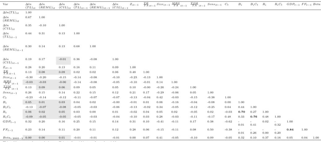
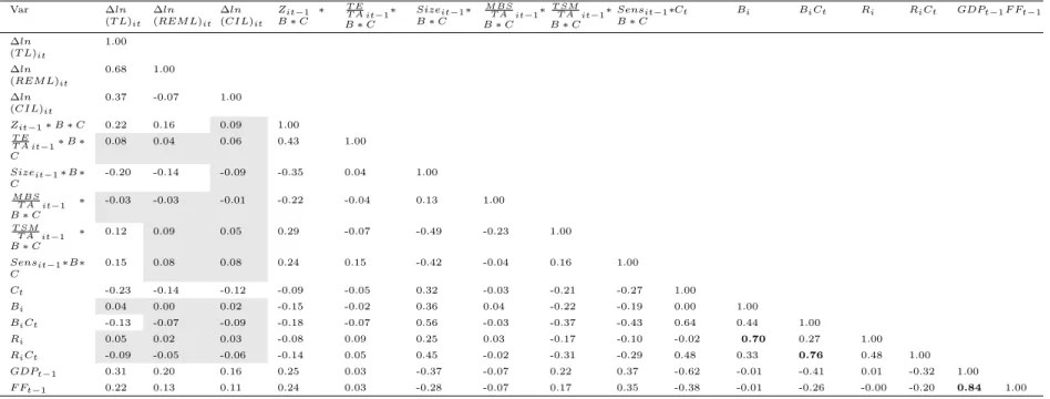
Table 4: Correlation coefficients for within-transformed dependent and main explanatory variables with no interactions Var ∆ln (T L)it ∆ln (REM L)it ∆ln (CIL)it ∆ln (T L)it−1 ∆ln (REM L)it−1 ∆ln (CIL)it−1 Zit−1 T E
T A it−1Sizeit−1 M BST A it−1
T SM
T A it−1 Sensit−1 Ct Bi BiCt Ri RiCt GDPt−1 F Ft−1Beta
∆ln(T L)it 1.00 ∆ln (REM L)it 0.67 1.00 ∆ln (CIL)it 0.35 -0.10 1.00 ∆ln (T L)it−1 0.44 0.31 0.13 1.00 ∆ln (REM L)it−1 0.30 0.14 0.13 0.68 1.00 ∆ln (CIL)it−1 0.19 0.17 -0.01 0.36 -0.08 1.00 Zit−1 0.28 0.20 0.13 0.16 0.11 0.09 1.00 T E T A it−1 0.13 0.08 0.09 0.02 0.02 0.06 0.48 1.00 Sizeit−1 -0.30 -0.20 -0.15 -0.14 -0.08 -0.10 -0.23 -0.13 1.00 M BS T A it−1 -0.03 -0.03 -0.00 -0.14 -0.08 -0.05 -0.10 -0.01 0.14 1.00 T SM T A it−1 0.13 0.09 0.06 0.09 0.05 0.05 0.10 -0.00 -0.26 -0.24 1.00 Sensit−1 0.26 0.15 0.14 0.22 0.15 0.12 0.21 0.17 -0.29 -0.06 0.05 1.00 Ct -0.23 -0.14 -0.12 -0.11 -0.07 -0.07 -0.13 -0.04 0.42 -0.03 -0.15 -0.38 1.00 Bi 0.05 0.01 0.03 0.04 0.02 -0.00 -0.01 0.01 0.06 -0.16 -0.04 -0.08 0.00 1.00 BiCt -0.13 -0.07 -0.08 -0.05 -0.03 -0.06 -0.13 -0.02 0.34 -0.05 -0.12 -0.25 0.64 0.44 1.00 Ri 0.06 0.02 0.05 0.03 0.00 0.01 -0.02 0.04 0.05 0.02 -0.05 0.02 -0.03 0.70 0.27 1.00 RiCt -0.09 -0.05 -0.05 -0.05 -0.03 -0.04 -0.10 0.03 0.28 -0.03 -0.11 -0.17 0.48 0.33 0.76 0.48 1.00 GDPt−1 0.32 0.20 0.16 0.25 0.15 0.14 0.31 0.10 -0.41 -0.11 0.17 0.38 -0.62 -0.01 -0.41 0.02 -0.32 1.00 F Ft−1 0.23 0.14 0.11 0.20 0.11 0.12 0.28 0.06 -0.15 -0.11 0.08 0.50 -0.38 -0.01 -0.26 -0.00 -0.20 0.84 1.00 Betai,2002−20070.00 0.00 0.01 -0.01 -0.01 -0.01 0.00 0.07 0.41 -0.05 -0.10 0.09 -0.05 0.32 0.10 0.37 0.16 0.05 0.04 1.00
This table reports the correlation coefficients for within-transformed variables.
The correlation coefficients between dependent and explanatory variables smaller than 0.1 in their absolute values are highlighted in grey.
26 Documents de Travail du Centre d'Economie de la Sorbonne - 2014.62
those of smaller banks during the crisis due to their greater exposure to the market of derivatives.
• Mortgage-Backed Securities (MBS)
There are two proxies for the level of liquidity that are considered in this model. Both are included in the liquidity indicator proposed by the Moody’s RiskCalc v3.1 U.S. Banks model (Dwyer et al., 2006). However, here it is suggested to distinguish between mortgage-backed securities and treasury and municipal securities due to their different positions during the recent crisis.
Moody’s RiskCalc v3.1 U.S. Banks model (Dwyer et al., 2006) and Basel II regula-tion classified mortgage-backed securities (MBS) as safe and liquid holdings. That was indeed the case at the time, MBSs also included government mortgages provided by Government National Mortgage Association or other U.S. Federal agencies. In normal times MBS were highly liquid assets that were widely traded, while with accelerat-ing speed of subprime defaults and consequential foreclosures significant part of them became highly risky or even ”toxic”.
Mortgage-backed securities in levels are normalised by total assets and are expected to positively affect loan growth rates before 2008 but negatively during the crisis. After 2008 MBS are expected to become a financial burden on the balance sheet of the banks that might lead to the scarce credit offer by such banks.
The correlation tables 4, 5 and 6, however, suggest only a weak correlation between the share of MBS in total assets and loan growth rates (-0.03, table 4). Thus, when choosing between MBS and the share of Treasury securities in the bank portfolio, the latter one is selected for the inclusion in final regressions.
• Treasury and Municipal Securities (TSM) include the loans made to federal, state and/or municipal government. As they represent the government debt issued by the U.S. Treasury, that type of securities remained the most liquid and secure during the crisis. The ”flight to security” that occurred due to the turbulence at the financial markets only strengthened the position of government-issued debt. Thus, the banks with larger amounts of Treasury and municipal securities in their asset portfolios had stronger and more liquid positions during the crisis, that could be translated into the more intensive lending activity. The correlation coefficients from tables 4, 5 and 6 between dependent variables and the shares of Treasury securities confirm that argument. Correlation with growth rates of total loans reaches 0.13 in normal times, 0.15 in crisis period and 0.11 for the bailed-out banks (tables 4, 5 and 6 respectively).
Table 5: Correlation coefficients for within-transformed dependent and main explanatory variables interacted with crisis dummy Var ∆ln (T L)it ∆ln (REM L)it ∆ln (CIL)it Zit−1 ∗ C T E T A it−1∗ C Sizeit−1∗ C M BS T A it−1∗ C T SM T A it−1∗ C Sensit−1∗ C Ct Bi BiCt Ri RiCt GDPt−1F Ft−1 ∆ln (T L)it 1.00 ∆ln (REM L)it 0.68 1.00 ∆ln (CIL)it 0.37 -0.07 1.00 Zit−1∗ C 0.25 0.18 0.11 1.00 T E T A it−1∗ C 0.13 0.08 0.09 0.49 1.00 Sizeit−1∗ C -0.28 -0.20 -0.14 -0.29 -0.07 1.00 M BS T A it−1∗ C -0.04 -0.05 -0.00 -0.12 0.02 0.13 1.00 T SM T A it−1∗ C 0.15 0.10 0.07 0.17 -0.07 -0.38 -0.23 1.00 Sensit−1∗ C 0.21 0.12 0.12 0.21 0.23 -0.38 -0.04 0.09 1.00 Ct -0.23 -0.14 -0.12 -0.09 -0.07 0.46 0.00 -0.28 -0.37 1.00 Bi 0.04 0.01 0.02 -0.06 0.03 0.09 -0.01 -0.04 -0.01 0.01 1.00 BiCt -0.13 -0.07 -0.09 -0.12 -0.02 0.37 -0.03 -0.21 -0.25 0.64 0.44 1.00 Ri 0.05 0.02 0.03 -0.02 0.10 0.06 -0.01 -0.04 0.02 -0.02 0.70 0.27 1.00 RiCt -0.09 -0.05 -0.06 -0.09 0.05 0.31 -0.03 -0.18 -0.16 0.49 0.33 0.76 0.48 1.00 GDPt−1 0.31 0.20 0.16 0.30 0.10 -0.52 -0.10 0.29 0.49 -0.62 -0.01 -0.41 0.01 -0.32 1.00 F Ft−1 0.22 0.13 0.11 0.29 0.09 -0.39 -0.10 0.21 0.46 -0.38 -0.01 -0.26 -0.00 -0.20 0.84 1.00 The correlation coefficients between dependent and explanatory variables smaller than 0.1 in their absolute values are highlighted in grey.
28 Documents de Travail du Centre d'Economie de la Sorbonne - 2014.62
Table 6: Correlation coefficients for within-transformed dependent and main explanatory variables interacted with bailout dummy Var ∆ln (T L)it ∆ln (REM L)it ∆ln (CIL)it Zit−1 ∗ B T E T A it−1∗ B Sizeit−1∗ B M BS T A it−1∗ B T SM T A it−1∗ B Sensit−1∗ B Ct Bi BiCt Ri RiCt GDPt−1F Ft−1 ∆ln (T L)it 1.00 ∆ln (REM L)it 0.68 1.00 ∆ln (CIL)it 0.37 -0.07 1.00 Zit−1∗ B 0.22 0.16 0.10 1.00 T E T A it−1∗ B 0.10 0.06 0.08 0.46 1.00 Sizeit−1∗ B -0.24 -0.16 -0.11 -0.24 -0.07 1.00 M BS T A it−1∗ B -0.02 -0.02 0.00 -0.14 -0.02 0.13 1.00 T SM T A it−1∗ B 0.11 0.07 0.04 0.15 0.05 -0.38 -0.22 1.00 Sensit−1∗ B 0.19 0.10 0.11 0.23 0.12 -0.32 -0.04 0.10 1.00 Ct -0.23 -0.14 -0.12 -0.13 -0.03 0.30 -0.06 -0.12 -0.28 1.00 Bi 0.04 0.00 0.02 0.05 -0.02 0.32 0.01 -0.24 -0.11 0.00 1.00 BiCt -0.13 -0.07 -0.09 -0.15 -0.05 0.52 -0.07 -0.25 -0.40 0.64 0.44 1.00 Ri 0.05 0.02 0.03 0.02 0.03 0.25 0.02 -0.20 -0.05 -0.02 0.70 0.27 1.00 RiCt -0.09 -0.05 -0.06 -0.11 0.03 0.42 -0.05 -0.22 -0.28 0.49 0.33 0.76 0.48 1.00 GDPt−1 0.31 0.20 0.16 0.26 0.04 -0.30 -0.07 0.13 0.44 -0.62 -0.01 -0.41 0.01 -0.32 1.00 F Ft−1 0.22 0.13 0.11 0.22 0.00 -0.12 -0.08 0.05 0.38 -0.38 -0.01 -0.26 -0.00 -0.20 0.84 1.00 The correlation coefficients between dependent and explanatory variables smaller than 0.1 in their absolute values are highlighted in grey.
29 Documents de Travail du Centre d'Economie de la Sorbonne - 2014.62
3.3.2 Sensitivity to demand shock on bank products
Most of the literature on bank lending including Brei et al. (2011); Berrospide and Edge (2010) focuses on the financial determinants of the bank credit supply. Demand factors are mostly captured via inclusion of the GDP growth rate, inflation and interest rates and other aggregate macroeconomic characteristics. In this article one of the core determinants of the credit supply are heterogeneous reactions of financial institutions to the shock on aggregate demand. These individual bank sensitivities allow to gauge the impact of decline in demand for credits on the bank loan growth.
First the cross-sectional demand sensitivities are constructed following Claessens et al. (2012). Each bank’s net income growth is regressed on the change in real GDP of the state where the bank is headquartered (in the period between 1990 and 2006):
∆N Ii,1990−2006 = αi+ βi∆ ln(RGDPST,1990−2006) + ǫi,1990−2006 (10)
where βi = ǫGDP = ǫ ∆N Ii,1990−2006 ∆RGDPST,1990−2006
is the slope or sensitivity of change in bank’s net income to real GDP growth in the state where the bank is headquartered. The alternative measure of this index contains the data on personal income instead of real GDP.
The idea beyond the first step is to estimate the impact of an increase in real GDP on bank revenues during 16 years prior to crisis. Secondly, the cross-sectional sensitivity is converted into individual bank sensitivity by multiplying the βi10 estimated from Equation
10 by annual real GDP growth of the state where the bank is headquartered ∆ ln(GDPST,t).
The correlation coefficients from table 4 confirm that sensitivity to demand shock is highly and positively correlated with growth rates of TL, REML and CIL (the coefficients are 0.26, 0.15 and 0.14, respectively, table 4).
3.4
Dummies and macroeconomic variables
• Dummies
– Crisis dummy is the dummy that takes on a value of 1 in the period from 2008 until 2011. It is longer than the conventional view on the crisis mostly suggests (between 2008-2009). Nevertheless, here the period is extended in order to capture the post-crisis period with sluggish economic growth during which the banks were supposed to recover and to support the credit offer to enterprises and individuals. Each bank-specific variable is interacted with the crisis dummy and both bailout
10
and crisis dummy (or repayment and crisis dummy for Model 2). The dummy itself and its interactions with other dummies are also included in the regressions. – Bailout dummy is the dummy that takes on two values, 0 and 1 (see table 2) to distinguish between the banks that did not receive CPP funds and those that did. Banks that have finally received CPP funds applied for Capital Purchase Program (CPP), have been approved for funding and then accepted the funds. Out of around 600 banks in the sample approximately 318 banks did not receive the CPP funds, while around 278 banks did.
– Repayment dummy is the binary variable that is equal to 1 if the bailed-out bank had repurchased its stake from the U.S. Treasury by July 2012; 0 otherwise. Regressions with repayment dummy and interactions of the bank-specific variables with that dummy are only run on the limited sample of bailed-out banks. 169 banks out of 278 banks (more than 60%) which received the CPP funds have reimbursed it by July 2012.
• Macroeconomic variables
– Real annual GDP growth accounts for time-fixed effects in the sample. The lending activity of the banks is expected to expand in the years with higher rates of production growth reflecting increasing population wealth and improvement of the state of economy in general.
– Change in 3-months London Interbank Overnight Rate (LIBOR) reflects the ten-dencies and changes in macroeconomic policies that are spilled over to the inter-bank markets. It is a principal component of the inter-bank lending channel literature that discusses the short-term effects of monetary policies on the changes in bank lending. Banks borrowing from the central bank or from the interbank markets, in case of abundant capital and low interest rates, tend to lower the interest rates on credits that in turn leads to higher investments and more intensive bank lending activity. The effect is the opposite in case of a rise of the interest rates.
However, these two macroeconomic variables cannot be included simultaneously in the regressions due to the high correlation between them (it reaches 0.84, table 4). That correlation arises due to the countercyclical nature of monetary policy: the central bank tends to increase the interest rates in the periods of intensive growth and to lower the interest rates during the recession. Hence, most of the regressions are conducted including only GDP growth.


![[PDF] Langage Python cours de base avec exemples | Formation informatique](data:image/gif;base64,R0lGODlhAQABAIAAAP///wAAACH5BAEAAAAALAAAAAABAAEAAAICRAEAOw==)