HAL Id: tel-03035021
https://tel.archives-ouvertes.fr/tel-03035021
Submitted on 2 Dec 2020HAL is a multi-disciplinary open access
archive for the deposit and dissemination of sci-entific research documents, whether they are pub-lished or not. The documents may come from teaching and research institutions in France or abroad, or from public or private research centers.
L’archive ouverte pluridisciplinaire HAL, est destinée au dépôt et à la diffusion de documents scientifiques de niveau recherche, publiés ou non, émanant des établissements d’enseignement et de recherche français ou étrangers, des laboratoires publics ou privés.
Particle methods in finance
Shohruh Miryusupov
To cite this version:
Shohruh Miryusupov. Particle methods in finance. Computational Finance [q-fin.CP]. Université Panthéon-Sorbonne - Paris I, 2017. English. �NNT : 2017PA01E069�. �tel-03035021�
T
H
E
S
E
Centre d’économie de la Sorbonne
Labex RéFi
Doctorat en Mathématiques Appliquées
THÈSE
pour obtenir le grade de docteur délivré par
Université Paris 1 Panthéon-Sorbonne
Spécialité doctorale “Sciences, technologies, santé”
présentée et soutenue publiquement par
Shohruh M
IRYUSUPOV
le 20 décembre 2017
Particle Methods in Finance
Directeur de thèse : Raphael DOUADY
La présidente : Dominique GUEGAN
Jury
M. Rama Cont, Professeur Rapporteur
M. Andrew Mullhaupt, Professeur Rapporteur
M. Pierre Del Moral, Directeur de Recherche Examinateur
M. Ricadro Perez-Marco, Directeur de Recherche Examinateur
M. Jean-Paul Laurent, Professeur Examinateur
Université Paris 1 Panthéon-Sorbonne Centre d’économie de la Sorbonne (CES)
Résumé
This thesis consists of two parts, namely rare event simulation and a homotopy trans-port for stochastic volatility model estimation.
Particle methods, that generalize hidden Markov models, are widely used in different fields such as signal processing, biology, rare events estimation, finance and etc. There are a number of approaches that are based on Monte Carlo methods that allow to ap-proximate a target density such as Markov Chain Monte Carlo (MCMC), sequential Monte Carlo (SMC). We apply SMC algorithms to estimate default probabilities in a stable pro-cess based intensity propro-cess to compute a credit value adjustment (CVA) with a wrong way risk (WWR). We propose a novel approach to estimate rare events, which is based on the generation of Markov Chains by simulating the Hamiltonian system. We demonstrate the properties, that allows us to have ergodic Markov Chain and show the performance of our approach on the example that we encounter in option pricing.
In the second part, we aim at numerically estimating a stochastic volatility model, and consider it in the context of a transportation problem, when we would like to find "an optimal transport map" that pushes forward the measure. In a filtering context, we understand it as the transportation of particles from a prior to a posterior distribution in pseudotime. We also proposed to reweight transported particles, so as we can direct to the area, where particles with high weights are concentrated. We showed on the example of Stein-Stein stochastic volatility model the application of our method and illustrated the bias and variance.
Keywords : Hamiltonianflow Monte Carlo, Particle Monte Carlo, Sequential Monte Carlo, Monte Carlo, rare events, option pricing, stochastic volatility, optimal transport
Table des matières
Table des matières iii
Liste desfigures v
Liste des tableaux vii
1 Introduction 1
1.1 Motivation . . . 2
1.2 Sampling Methods . . . 5
1.3 Particle Methods and Sequential Monte Carlo . . . 6
1.4 Hamiltonian Flow Monte Carlo . . . 10
1.5 Filtering by Optimal Transport . . . 13
1.6 Organinzation of the thesis and main contributions . . . 14
2 Particle Levy temperedα-stable credit risk model simulation with application to CVA with WWR computation in multi-factor BGM setting 21 2.1 Introduction . . . 24
2.2 Problem Formulation and Definitions . . . 24
2.3 Market Risk and Exposure Profiles . . . 25
2.4 Credit Risk . . . 27
2.5 WWR Modelling . . . 37
2.6 Particle Interpretations . . . 37
2.7 Numerical Analysis and Discussion . . . 44
2.8 Conclusion . . . 52
3 Hamiltonianflow Simulation of Rare Events 55 3.1 Introduction . . . 57
3.2 Monte Carlo and Interacting Particle System . . . 57
3.3 Hamiltonian flow Monte Carlo . . . 59
3.4 Convergence Analysis . . . 65
3.5 Applications and Numerical Results . . . 67
3.6 Conclusion and Further Research . . . 69
4 Optimal Transport Filtering with Particle Reweighing in Finance 73 4.1 Introduction . . . 75
4.2 Particle Filtering . . . 75
4.3 Homotopy Transport . . . 79
4.4 Homotopy Transport with Particle Reweighing . . . 83
4.5 Numerical Applications and Results . . . 85
Liste des
figures
1.1 HMC sampling from Bivariate Gaussian distribution . . . 13 2.1 Left : Positive exposure profiles. Right : EPE(Blue), ENE(Red) . . . 27 2.2 The paths of CIR process (left) and survival function (right) . . . 28 2.3 OU Jump-diffusion process with exponentially tempered α-stable jumps (left),
Survival probability (right) with α =0.8 . . . 35 2.4 OU Jump-diffusion process with exponentially tempered α-stable jumps (left),
Survival probability (right) with α =1.5 . . . . 36 2.5 PMC simulation of OU Jump-diffusion process with exponentially tempered
α-stable jumps (left), Survival probability (right) with α =0.8 . . . . 43 2.6 PMC Euler, Euler jump-adapted, Milstein jump-adapted strong errors, α =
0.8, #(particles)=1000. . . 45 2.7 MC vs PMC Euler (left) and jump-adapted (right) strong errors. α =0.8, #(particles)=
1000, #(simulated paths)=5000 . . . 46 2.8 MC vs PMC Euler/Milstein (left) and jump-adapted (right) paths. α =1.5,
#(particles)=1000, #(simulated paths)=5000 . . . . 47 2.9 EPE profile of the LIBOR swap (left), CVA process (right) . . . 49 4.1 Volatily dynamics, PF (Blue), Homotopy (Red), RW-homotopy(Yellow) . . . 86 4.2 Zoomed volatilty dynamics. Homotopy (left), RW-homotopy (right) . . . 87
Liste des tableaux
2.1 ||·||L2error estimates of numerical schemes using MC and PMC density
ap-proximations, α =0.8 . . . 44 2.2 ||·||L1error estimates of numerical schemes using MC and PMC density
ap-proximations . α =0.8 . . . . 44 2.3 ||·||L2error estimates of numerical schemes using MC and PMC density
ap-proximations, α =1.5 . . . 44 2.4 ||·||L1error estimates of numerical schemes using MC and PMC density
ap-proximations . α =1.5 . . . 45 2.5 CVA WWR/free for LIBOR SWAP. PMC approach. α =0.8, #(scenar i os) := #(sc) 51 2.6 LIBOR SWAP CVA WWR/free for different values of ρ and λ0, α =0.8. PMC
approach. . . 51 2.7 LIBOR SWAP CVA WWR/free for different values of ρ and λ0, α =0.8. PMC
approach. . . 51 3.1 DOC Barrier option estimates statistics. B =65,X0=100, K =100, r =0.1,σ =
0.3, T = 1/2, and di v =0; δ = 0.0001, #(Leap frog step) : 35. True price : 10.9064, nS=50000, nt=750 . . . 69 3.2 DOC Barrier option estimates statistics. B =65,X0=100, K =100, r =0.1,σ =
0.3, T = 1/2, and di v =0; δ = 0.0009, #(Leap frog step) : 40. True price : 10.9064, nS=75000, nt=750 . . . 69 4.1 Stein-Stein Stochastic volatility option price estimates statistics. S0=100, K =
90, r =0.0953,σ =0.2, κ =4, θ =0.25, V0=0.25, T =1/2, and dividends d =0 True price :16.05, t =20000, M =64 . . . 86 4.2 Stein-Stein Stochastic volatility option price estimates statistics. S0=100, K =
90, r =0.0953,σ =0.2, κ =4, θ =0.25, V0=0.25, T =1/2, and dividends d =0 True price :16.05, t =40000, M =64 . . . 87
Chapitre 1
Introduction
« " πάντες ˝αντροποι τοˆυ είδέναι ˙ ορέιγονται ϕύσει. τὰ μετά τὰ ϕισικά ’» Αριστοτέλη« "All men by nature desire to
know" »
Aristotle
Sommaire
1.1 Motivation . . . . 2
1.1.1 Credit Risk Estimation . . . 2
1.1.2 Pricing in Partial Observation Models . . . 4
1.2 Sampling Methods . . . . 5
1.2.1 Monte Carlo . . . 5
1.2.2 Importance Sampling . . . 5
1.2.3 Markov Chain Monte Carlo . . . 5
1.3 Particle Methods and Sequential Monte Carlo . . . . 6
1.3.1 Feynman-Kac Approximations . . . 7
1.3.2 Hidden Markov Models . . . 7
1.3.3 Sequential Monte Carlo . . . 8
1.4 Hamiltonian Flow Monte Carlo . . . 10
1.4.1 Sampling with HFMC . . . 10
1.5 Filtering by Optimal Transport . . . 13
CHAPITRE 1. INTRODUCTION
1.1 Motivation
Throughout last 20 years development of computation power allowed to use sophisti-cated Monte Carlo methods in signal-processing, rare events estimation, computational biology, queuing theory, computational statistics and etc. In finance we have to deal with large dimensionality of problems, where other techniques due to some constraints, such as curse dimensionality, computational burden makes us to look for alternative numeri-cal techniques. Particle methods are a broad class of interacting type Monte Carlo algo-rithms for simulating from a sequence of probability distributions satisfying a nonlinear evolution equation. These flows of probability measures can always be interpreted as the distributions of the random states of a Markov process whose transition probabilities de-pends on the distributions of the current random states ([6], [5]).
Particle methods have a variety of applications in finance : rare events and stochastic volatility estimation. For instance, portfolio managers need to estimate a large portfolio loss for risk management. In banking industry, banks need to compute default probabi-lities, so as to compute different value adjustments and to comply with financial regula-tion. In insurance industry, companies are interested in estimating ruin probabilities in a given time horizon. All the above mentioned cases are the examples, where rare event simulation is applied.
Stochastic volatility models are widely used in the financial industry. In fact, while rea-lized volatility could be hedged away by trading other options, stochastic volatility models are needed to model the dynamics of implied volatilities, which will provide their user with simple break-even accounting conditions for the Profit and Loss of a hedged posi-tion [1].
The current thesis consists of two main parts, namely computing rare events via simu-lation and general stochastic volatility estimation.
1.1.1 Credit Risk Estimation
Since the credit crisis 2007-2009, the importance of counterparty credit risk for regu-lators increased dramatically. According to Basel III regulation [33], banks are required to hold a regulatory capital based on CVA charges against each of their counterparties. The is already a number of article on CVA valuation, the most common Credit Value Adjustment (CVA) formula ([5], [22], [22], [39] and [40]) is given by :
CVA = (1− R) ∫T
0
DtE[V+t |τ = t]dPD(t) (1.1)
where R is a recovery rate, Dt - risk-free discount rate, PD(t) probability of default up to
time t and Vt - the value of an underlying asset.
Two problems related to CVA computation that usually arise : incorporation of wrong way risk (WWR) into the value of CVA and a high computational burden. WWR is a sta-tistical dependence between the exposure and a counterparty’s credit risk (CCR). Another challenge related to CVA is the computation of default probability. There are two main ap-proaches in default probability computation : structural models (first-passage approach) [3] and reduced form credit models ([19], [26] and [28]).
CHAPITRE 1. INTRODUCTION
Structural models
The first passage approach is modelled like in a barrier option pricing, and formulated in the following way. Assume that the default barrier b is constant valued. Then the default time τ is a continuous random variable (r.v.) values in ]0,+∞[ and given by
τ = inf{t >0: Vt< b} (1.2)
then the first passage probability is given by : P(T) = P(MT< b) = P(inf s≤T ( µs+ σDWs ) < log(b/V0)) (1.3) where MT= infs≤TVs. Default intensity
The main difference between reduced form and structural models is in the fact that, in the latest one does not need any economic model of firm’s default, i.e. defaults are exogenous.
Dt= 1τ<t=
{ 1 if
τ≤ t
0 otherwise (1.4)
Observe that default intensity is an increasing process, such that the conditional proba-bility at time t that the firm defaults at time s ≥ t is at least as big as the process Dt.
A process with such property is called submartingale. The Doob-Meyer decomposition theorem says that we can isolate upward trend from D. This very important result says that there exist an increasing process Dτstarting at zero such that D − Aτbecomes a
mar-tingale. The unique process Aτcounteracts the upward trend in D, and it is called a
com-pensator. It describes the cumulative and conditional likelihood of default, which is para-meterized by non-negative process λ.
Aτ t = ∫tτ 0 λs d s = ∫t 0 λs 1τ>sd s (1.5)
where λt describes conditional default rate for small interval∆t andτ > t. λ∆t
approxi-mates the probability that default occurs in the interval ]t, t +∆t ].
Rare events
Rare events simulation is an important field of research in computational and nume-rical probability. It has a wide range of applications starting from catastrophe theory to finance, as an example one can consider pricing of a barrier option pricing or a credit risk estimation.
Let us consider the problem of rare event estimation, where the probabilityz= P(A) is very small. The crude Monte Carlo (CMC) estimateszthrough the proportion of times on the simulated points attain rare event area A over M independent trials :
bzM= 1 M M ∑ m=1 1ξ(m)∈A (1.6)
with variance σ = √z(1−z). In "easy problems" we can use the central limit theorem (CLT), which asserts that
1 p
CHAPITRE 1. INTRODUCTION
where Z ∼ N (0,1) is a standard Gaussian distribution.
In a rare-events simulation we are not very concerned about the absolute error, but instead we would like to measure via relative error(RE) the precision of our estimation with respect to some "true" value of quantity we are computing. Relative error exposes the problems one encounters by using CMC in rare event setting :
RE =Z √ z(1−z) M1/2 z = Z √ 1−z Mz ∝ Z √ Mz−−−→z→0 ∞ (1.8)
The approximation (1.8) shows that CMC requires n ≫1/z. Lets show this on a simple example, assume that we would like to estimate rare event probabilityz=10−7, RE is tar-geted at0.1with a95% confidence interval, then we have
1.96 p
10−7M≤
0.1 (1.9)
from the equation above we see that we need at least M ≥3.84×10⁻⁹ samples to have a 10% RE.
Assume that we have a sequence of random variables {ξ(a)(m)}Mm=1. Define the rare
event set as :
Aa= {x ∈ RM, f (x) > a} (1.10)
then we can define a probability of interest and its estimator as
z(a) = E[1ξ(a)∈Aa] and bz(a) =
1 M M ∑ m=1 1ξ(m)(a)∈Aa (1.11)
We can show that if our estimator has a bounded RE, then the desired precision is independent of that the rarity of the set Aa.
P (
|bz(a) −z(a)| z(a) > ϵ
)
≤Var (ξ(a))Mϵ2z(a)2 (1.12)
From the equation (1.12) we that the set will not depend on the "rarity" of the set Aa,
if we impose the following condition :
limsup
a→∞
Var (ξ(a))
z(a)2 < ∞ (1.13)
1.1.2 Pricing in Partial Observation Models
Stochastic volatility models are the one of examples of the use of partial observation models (hidden Markov models) in finance, i.e. the situation, when one can observe the prices but not the dynamics of the stochastic volatility. In the last chapter we will show the application of different numerical approaches, such as particle filtering and homo-topy transport on the example of a barrier option pricing in Stein-Stein stochastic volati-lity models. For example, in [1] author showed that the price of a barrier option is mostly dependent on the dynamics of the at-the-money skew conditional on price hitting the barrier. A stochastic volatility model for barrier options would need to provide a direct handle on this precise feature of the dynamics of the volatility surface so as to appropria-tely reflect its Profit and Loss impact in the option price. On of the first applications in option pricing could be found in [6]. Other applications and analysis of hidden Markov models could be found in [8] and [32].
CHAPITRE 1. INTRODUCTION
1.2 Sampling Methods
1.2.1 Monte Carlo
The application of CMC in a rare event setting was already demonstrated in previous sections. These methods are generally used to compute integral that can not be calcula-ted analytically or very difficult to compute. For example, we would like to calculte the following expectation :
EP[h(X)] = ∫
X
h(x)P(d x) (1.14) All we need is to generate M independent and identically distributed (i.i.d.) random va-riables {ξ(m)}Mm=1according to the law P. Using the law of large numbers (LLN) we have an
unbiased estimator 1 M M ∑ m=1 δξ(m)(x)h(x)−−−−→a.s. M→∞ E P[h(X)] (1.15)
As we saw in the previous section, often we can not efficiently sample from the measure P. Those problems arises in rare events setting and sampling from fat-tailed distributions, then we have to use advanced Monte Carlo techniques, such as an importance sampling (IS), control variates, a stratified sampling and etc.
1.2.2 Importance Sampling
One of the ways to deal with rare events probabilities is IS Monte Carlo method. The idea is to change a measure from P, where samples rarely reach rare event sets, to the measure Q, so that we can sample at low cost in the new measure .
EP[h(X)] = ∫ X h(x)P(d x) = ∫ X h(x)ω(x)Q(d x) = EQ[h(X)ω(X)] (1.16) M ∑ m=1 δξ(m)(x)ω(x)h(x)−−−−→a.s. M→∞ E Q[h(X)ω(X)] (1.17)
The disadvatage of this method is in the fact, that we do not know the explicit form of the Radon-Nykodim derivative d P
d Q= ω. This method is unfeasible in many examples, if we
exclude some simple cases.
1.2.3 Markov Chain Monte Carlo
Markov Chain Monte Carlo (MCMC) method allows to approximate a target measure π, by constructing an ergodic Markov Chain, that admits the target measure as a statio-nary law. We do not need to know the law explicitly as in the case of the IS, but instead we construct a Markov kernel K , that leaves the target measure π invariant. There are two very popular MCMC sampling techniques : Metropolis-Hastings(MH) and Gibbs al-gorithms. One can show that the Gibbs algorithm is a special case of MH. The idea behind Metropolis-Hastings algorithm is to propose new set of candidates, and accept them, so that the transition kernel K is left invariant with respect to the target, where Markov tran-sition kernel is given by :
K(x,d y) = α(x, y)Q(x,d y) + ( 1− ∫ α(x, z)Q(x, d z) ) δx(d y) (1.18)
CHAPITRE 1. INTRODUCTION
and MH transition kernel K is reversible, i.e. πK = π. By recursion we can show that the chain {Xn}n≥0follows the law πn= π0Kn. Using reversibility property of the kernel K , we
can have convergence of the chain Xn to the target measure π, given that the kernel K
has contraction :
πn− π = (π0− π)Kn∀n >0 (1.19)
If the chain Xlis irreducible, or in other words it admits a unique invariant measure, then
the paths of the chain satisfies ergordic theory :
lim n→∞ 1 n nH∑+n l =nH+1 h(Xl) = Eπ[h(X)] (1.20)
where nH is the number of iterations needed for "burn-out period", so that the chain
leaves its initial law, and converges to the invariant measure π. Usually one needs to make high number of iterations, so that MH algorithm will approach the target density.
The performance of MCMC algorithms, like in other Monte Carlo sampling algorithms depends on the experience and ability to tune and optimize it. In general, the quality of final samples depends on the kernel K and how fast it is able to explore the state space. In chapter 3 we will show, that the transition kernel represented by a metropolized Hamil-tonian dynamics allows to explore it fast.
Algorithm 1 : MH MCMC algorithm
1 Initialization : N - #(time steps), π0- initial measure
2 X0∼ π0;
3 for n =1,...,N do
4 Generate x∗from Q(·,Xn−1) ;
5 Compute the weight :
a(Xn, x∗) =1∧
π(x∗)q(x∗,Xn)
π(Xn)q(Xn, x∗)
assuming that a(x, y) =0if π(x)q(x, y) =0; 6 Drawu∼ U nif(0,1) ;
7 ifu< a then 8 Set Xn+1= x∗;
9 else
10 Reject, and set Xn+1= Xn
11 end
12 end 13 end
1.3 Particle Methods and Sequential Monte Carlo
Interacting particle system(IPS) is very power method, that is applied in non-linear filtering problems, rare event estimation and many other applications. IPS allows to over-come the problem that we face in importance sampling Monte Carlo technique, where we needed to know explicitly the importance sampling measure in order to sample from it. On contrary, the importance measure is approximated by a collection of trajectories of a Markov process {Xn}n≥0weighted by a set of potential functions ωn. IPS is related to the
unnormalized Feynman-Kac models. In the next section we give a brief overview of these stochastic models, for more details we refer to monographs [6] and [5].
CHAPITRE 1. INTRODUCTION
1.3.1 Feynman-Kac Approximations
We give some key notations that are used to describe Feynman-Kac models, that we use in the next chapters. First, we define normalised and unnormalized Feynman-Kac measures (ηn,γn) for any bounded function f by the formulae :
γN(f ) = E[f (XN) N−∏1
n=0
ωn(Xn)] and ηN(f ) = γN(f )
γN(1X) (1.21)
Since non-negative measures (ηn)n≥0 satisfy for any bounded function f the recursive
linear equation : γn(f ) = γn−1(Qn(f )) we have
γN(f ) = ∫ ... ∫ f (XN)η0(d x0) ∏ Qn(xn,d xn+1) (1.22)
where {Qn}n≥0are unnormalised transition kernels, for example, we can choose them of
the following form Qn(xn,d xn+1) = ωn(xn)kn(xn,d xn+1), where {kn}n≥0 is a sequence of
elementary transitions.
The following definition was given in [6], for a linear semigroup Qm,n,0≤ m ≤ n
asso-ciated with a measure γnand defined by : Qm,n= Qm+1,...,Qn. For any bounded function f and (m, n)∈ N : γn(f ) = γmQm...Qn−1f andηn(f ) = γmQm...Qn−1(f ) γmQm...Qn−1(1X) = ηmQm...Qn−1(f ) ηmQm...Qn−1(1X) (1.23)
with a convention Qm,...,Qn= Id, if m > n by definition of a normalised measure ηnand
a semigroup Qm,nwe readily obtain
ηn+1(f ) =
ηnQn(f )
ηnQn(1X) (1.24)
Let us consider the example of rare events estimation, assume that we have a sequence of rare event sets {Ap}0≤p≤n, X is a random variable on the probability space (Ω,P,F ).
One of the application in barrier option pricing or credit risk estimation is computation of conditional expectation
ηN(f ) = E[f (XN)|Xp∈ Ap] (1.25)
Feynman-Kac interpretation for any bounded function f and potential function ωn(x) =
1An(x), using the fact that 1An1An+1= 1An(x), since An+1⊂ An
ηN(f ) = 1 P(AN) ∫ 1AN(x)h(x)P(d x) = E[f (XN)∏N−l =11ωl(Xl)] E[∏N−1 l =1 ωl(Xl)] =E[f (XN)1AN(X)] E[1AN(X)] (1.26)
1.3.2 Hidden Markov Models
As we mentioned in the motivation section, hidden Markov Models (HMM) can be formulated in the context of a filtering problem. Under the filtering problem one assumes that we have a couple of processes in discrete time (Xn,Yn)n≥0, where (Xn)n≥0 is a
se-quence of hidden variables and (Yn)n≥0is partially observed data.
Xn+1|Xn= xn∼ kn(xn,d xn+1) (1.27)
CHAPITRE 1. INTRODUCTION
where knis an elementary transition kernel, and ρnis a likelihood function. Using Bayes
formula for a bounded function f we can derive
E[f (X0,...,Xn)|Y0,...,Yn−1] =
∫
...∫f (X0,...,Xn)∏ρp(Xp,Yp)ν(d x0)k0(X0,d x1)...kn−1(Xn−1,d xn)
∫
...∫∏ρp(Xp,Yp)ν(d x0)k0(X0,d x1)...kn−1(Xn−1,d xn)
(1.29) Motivating example for studying and using HMM in finance is stochastic volatility model. It is defined by the following system :
d Yt= µ(Xt)d t + σY(Xt)dWt
d Xt= β(Xt)d t + σX(Xt)dBt (1.30)
Using Euler discretization scheme we have
Yn= Yn−1+ µ(Xn)∆t + σY(Xn) p ∆t Z(n1) Xn+1= Xn+ β(Xn)∆t + σX(Xn) p ∆t Z(n2) (1.31) where Z(1) and Z(2)
are two independent standard Gaussian r.v.,∆t is a discretization step.
In this case, the unnormalised transition kernel has the following form Qn(xn,d xn+1) =
ρn(xn,d yn)kn(xn, xn+1). For the sake of illustration, assume that we have constant
vola-tilities σX(Xn) = σX, σY(Xn) = σY, and other parameters are given by ∆t =1, β(Xn) =0,
µ(Xn) = Xnand Yn−1=0, then the likelihood is given by
ρn(xn,d yn) = 1 p 2πσYexp ( −(yn− xn) 2 2σ2 Y ) (1.32)
and an elementary Markov transition kernel
kn(xn,d xn+1) = 1 p2 πσX exp ( −(xn+1− xn) 2 2σ2 X ) (1.33)
If we exclude toy examples, there does not exist the exact simulation method for such type of models. Sequential Monte Carlo based particle algorithms allow to approximate normalised measures ηn.
1.3.3 Sequential Monte Carlo
Assume that on the measurable space (X,X ), there exists an unnormalized transition Qn : Xn× Xn → R+, which is absolutely continuous with respect to a kernel Kn : Xn× Xn+1→ R
+, i.e. Qn(xn,·) ≪Kn(xn,·) for all xn ∈Xn, then we can define an importance
weight function ωn:
ωn(xn, xn+1) =
d Qn(xn,·)
dKn(xn,·)
(xn+1) (1.34)
Sequential Monte Carlo (SMC) produces a fixed number of weighted samples (particles). At each time instant we generate a couple of particles and their corresponding weights {ξm
n,ω(m)n }Mm=1, where M is a fixed number of particles. If at time n ∈ N, the set of
weigh-ted particles {ξ(m)n ,ω(m)n }Mm=1approximates measure ηn, then using IS method, we can also
approximate ηn+1 by a couple of the set of particles and their corresponding weights.
{ξ(m)n+1,ω
(m)
CHAPITRE 1. INTRODUCTION
allows us recursively construct the measure ηN from the initial measure η0∈ P (X) and
the set of importance weights {ω(m)n }Mm=1.
Algorithm 2 : Sequential Importance Sampling algorithm
1 Initialization : M - #(simulations), N - #(time steps), η0- initial measure
2 for m =1,...,M do 3 ξ(m)0 ∼ η0; 4 ξ(m)1 ∼K0(ξ(m)0 ,·) ; 5 ω(m)1 = ω(m)0 (ξ(m)0 ,ξ(m)1 ) 6 end 7 for n =1,...,N do 8 for m =1,...,M do
9 Generate ξ(m)n fromKn(·,ξ(m)n−1) and set bξ
(m)
n = (bξ(m)n ,ξ(m)n−1) ;
10 Compute the weight : ω(m)n (bξ(m)n ) ; 11 end
12 end
In some cases, we can observe the weight degeneracy, when the variance of impor-tance weights increase over time, as the fact that most of weights are negligible. To over-come this problem, in [24] authors proposed to resample particles at each iteration, which was called sequential importance resampling (SIRS) or bootstrap algorithm. There was an extensive research to optimize the bootstrap using, for example, effective sample size (ESS), we refer to [27], [16] and [14] for details.
In [6] and in [5] it was shown, that SMC estimators are unbiased, i.e. we can prove that
sup ||f ||≤1 ¯ ¯ ¯ ¯ ¯ ¯ ¯ ¯ ¯ ¯E [ 1 M M ∑ m=1 f (ξmN) − ηN(f ) ]¯¯ ¯ ¯ ¯ ¯ ¯ ¯ ¯ ¯≤ c(N) M (1.35)
where c(N) is some positive constant, whose values depend on time horizon N.
Algorithm 3 : Sequential Importance Resampling algorithm
1 Initialization : M - #(simulations), N - #(time steps), η0- initial measure
2 for m =1,...,M do 3 ξ(m)0 ∼ η0; 4 ξ(m)1 ∼K0(ξ(m)0 ,·) ; 5 ω(m)1 = ω(m)0 (ξ(m)0 ,ξ(m)1 ) 6 end 7 for n =1,...,N do 8 for m =1,...,M do 9 if n < N then
10 Resample using probability weight : Wn(bξ(m)n ) =
ωn(bξ(m)n ) 1 M∑Mj =1ωn(bξ (j ) n ) ; 11 end
12 Generate ξ(m)n fromKn(·,ξ(m)n−1) and set bξ
(m)
n = (bξ(m)n ,ξ(m)n−1) ;
13 Compute the weight : ω(m)n (bξ(m)n ) ; 14 end
CHAPITRE 1. INTRODUCTION
1.4 Hamiltonian Flow Monte Carlo
Hamiltonian Flow Monte Carlo (HFMC) methods came from statistical physics, where the computation of macroscopic properties requires sampling phase space configura-tions distributed according to some probability measure. One of its first application in sampling from high-dimensional distribution was proposed in [15], and its differenti ex-tensions and converging properties in [2], [12] and [6]. Sampling on Riemann manifolds using generalised HFMC was introduced in [14].
We consider the system of particles described by a position and momentum X and P respectively, that are modelled by a Hamiltonian energy H (X,P). In statistical physics, the macroscopic properties can be obtained by averaging of some function A with respect to a probability measure P describing the state of the system of particles :
EP[A(X)] = ∫
X
A(x, p)P(d x,d p) (1.36)
In most cases we approximate the above expectation numerically, such that as number of iteration increases, the microscopic sequences converge to the target distribution P :
lim N→∞ 1 N N−∑1 i =0
A(Xn,Pn) = EP[A(X)] P − a.s. (1.37)
One of the simplest examples are so called canonical measures that have the following form : P(d x,d p) = 1 Ze −βH (x,p)d xd p, Z =∫ X e−βH (x,p)d xd p (1.38)
The measure P is called Gibbs measure. Since we can separate potential and kinetic ener-gies in the Hamiltonian, we can consider positions sampling, by using projection opera-tor.Define the projection operator as pr o j ◦P(dx,dp) = P(dx), and consider the canonical measure, ν, which is a projection of P.
ν(d x) = 1 Ze
−βΨ(x)d x, Z =∫
X
e−βΨ(x)d x (1.39)
If the Hamiltonian is separable, then the measure P takes tensorized form, and each element of momenta follows independent Gaussian distributions. The main difficulty, that one encounters in computational statistics, biology is sampling of potential energy. The approaches to sample new configurations are as follows :
— "Brute force" sampling methods, such as rejection sampling
— MCMC techniques, when we accept or reject new proposals using MH algorithm — Markovian stochastic dynamics, when we generate new samples using Langevin
or generalized Langevin equations
— Deterministic methods on the extended state space
1.4.1 Sampling with HFMC
In chapter3we apply HFMC algorithms to estimate rare events. There are number of challenges to compute ensemble averages in eq. (1.37), for example the dynamics of Xn
is not ergodic with respect to the Gibbs measure, i.e. paths are not sampled from ν. The system can contain high energy barriers that will prevent fast sampling.
CHAPITRE 1. INTRODUCTION
A large deviation theory defines rare event, when the dynamics has to overcome a potential barrier∆Ψ, such that the exit time scales like
τ∝ exp(−β∆Ψ) (1.40)
We can interpet τ in the sense that sampling from the Gibbs measure takes exponentially long time. There is the following law of large numbers.
Theorem 1.4.1 [30] Givenτ sufficiently small, let the numerical flowΞτbe symmetric and symplectic. Then
Xn+1= (pr o j ◦Ξ)(Xn,Pn), Pn∝ e−βH (Xn,·) (1.41)
P(Xn+1= xn+1) =1∧ e−β∆
Hn+1 (1.42)
defines an irreducible Markov process {X0,X1,...} ⊂X with unique invariant probability measureπ and the property
1 N N ∑ n=1 f (Xn) → ∫ Ef dπ a.s., ∀X 0∈X (1.43)
One can simply understand the irreducibility property as the probability of reaching any point on the configuration space is nonzero, i.e.
P(Xn+1∈ B(xτ)|Xn= x0) >0 (1.44)
holds true ∀x0, xτ∈Xand any Borel set B = B(X).
In algorithm3, we show how we can sample using Hamiltonian dynamics, which consist of sampling new momenta proposals P according to the kinetic part of the canonical measure ; performing L steps of numerical integrationΞn, which is the discretized
ver-sion of Hamiltonian system, to obtain a new configuration (x∗,P∗) ; and finally computing
CHAPITRE 1. INTRODUCTION
a = min(1, pr ob).
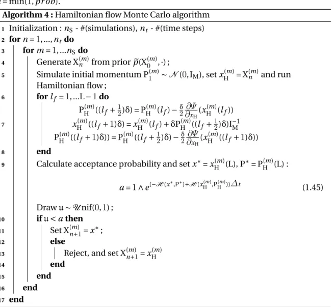
Algorithm 4 : Hamiltonianflow Monte Carlo algorithm 1 Initialization : nS- #(simulations), nt - #(time steps)
2 for n =1,...,nt do 3 for m =1,...nSdo
4 Generate X(m)n from prior ep(X(m)0 ,·) ;
5 Simulate initial momentum P1(m)∼ N (0,IM), set x(m)H = X(m)n and run
Hamiltonian flow ; 6 for lf =1,...L −1do 7 PH(m)((lf + 1 2)δ) = P (m) H (lf) −δ2∂∂Ψx H(x (m) H (lf)) xH(m)((lf +1)δ) = xH(m)(lf) + δP(m)H ((lf + 1 2)δ)I− 1 M P(m)H ((lf +1)δ)) = PH(m)((lf + 1 2)δ) − δ 2∂∂Ψx H(x (m) H ((lf +1)δ)) 8 end
9 Calculate acceptance probability and set x∗= xH(m)(L), P∗= PH(m)(L) :
a =1∧ e(−H (x∗,P∗)+H (xH(m),PH(m)))∆t (1.45) Drawu∼ U nif(0,1) ; 10 ifu< a then 11 Set X(m) n+1= x∗; 12 else
13 Reject, and set X(m)
n+1= x (m) H 14 end 15 end 16 end 17 end
As a simple example, consider sampling from a bivariate Gaussian distribution p(x) = N (µ,Σ) with mean and covariance matrix
µ = [ 0 0 ] , Σ= [ 1 0 .9 0.9 1 ] (1.46)
Then the potential energy function and partial derivatives are given by
Ψ(x) = −log(p(x)) = x TΣx 2 , ∂Ψ ∂xi = xi (1.47)
Figure 1.1 shows samples from bivariate Gaussian distribution. We see that HFMC fastly explores the state space and samples from a target distribution.
CHAPITRE 1. INTRODUCTION
FIGURE1.1 – HMC sampling from Bivariate Gaussian distribution
1.5 Filtering by Optimal Transport
In previous sections we showed how particle filters can be applied to approximate li-kelihood function by a set of weighted particles. It was shown in [1], [14], [15] that if the dimension of filtering problem increases, then the collapse of particles grows super - ex-ponentially. In [29], authors introduced a new approach to update system’s measurement, where the homotopy is formed, that gradually transforms an initial prior into a posterior density as scale parameter λ increases from0to1. The idea is to choose a parameterized density and minimize the deviation between this density and homotopy, according to the measure of deviation. The approach can be interpreted as the optimal transport problem, which is defined as :
infT E[||T (X) − X||2]
s. th. Q = T#P (1.48)
That means that we try to approximate some importance measure Q by an optimal trans-port map T , that minimize the deviation between particles transtrans-ported using the homo-topy and posterior distribution. Instead of approximating the likelihood function by a set of particles sampled through importance resampling algorithm, we find a transport map that moves random variables using the following homotopy :
ψ(Xt ,λ|Yt) =
1
Zλp(Xt ,λ|Yt−1)ρ(Yt|Xt ,λ)
λ (1.49)
The homotopy continuously deforms a prior distribution p(Xt|Yt−1) into an
unnormali-zed posterior p(Xt|Yt−1)ρ(Yt|Xt ,) as λ approaches to1:
ψ(Xt ,λ|Yt)
λ(0→1)
−−−−−→ ψ(Xt|Yt) (1.50)
The transportation of particles in nXdimensional state space is performed by a particle
flow. The idea is to find a flow of particles that correspond to the flow of probability den-sity defined by a homotopy. We suppose that flow of particles for Bayes rule follows the following dynamics in pseudo time λ :
CHAPITRE 1. INTRODUCTION
where g (Xt ,λ) =
d Xt ,λ
dλ .
In chapter4we will show that the flow g (x,λ) can be found as a solution to Fokker-Plank partial differential equations, given that its diffusion matrix sums to zero, the flow is given by : g (Xt ,λ) = [ ∂2Ψ(Xt ,λ) ∂X2 t ,λ ]−1[ ∂L(Xt ,λ) ∂Xt ,λ ]T (1.52)
Algorithm 5 : Homotopy Transport Algorithm
1 Initialization : i =1,...,nX- #(simulations), t =1,...,N - #(time steps) 2 Draw {X(i )0 }ni =X1from the prior p0(x).
3 Set {ω(i )0 }ni =X1=n1
X
4 for t =1,...,N do 5 for i =1,...,nXdo
6 Propagate particles using state equation X(i )t = f (X(i )t−1,Y(i )t−1,ϵt) ; 7 Measurement update : Yt= h(X(i )t ,Y(i )t−1,ηt) ; 8 Initialize pseudo-time λ =0; 9 Set X(i ) t ,λ= X (i ) t |n−1; 10 whileλ <1do 11 Compute SCM bSM; 12 Calculate an estimate : Xt ,λ= n1 X ∑ iX(i )t ,λ
13 Compute the matrix bH =∂
h(X(i )t ,λ)
∂Xt ,λ ;
14 Update the time : λ = λ +∆λ ;
15 Calculate the flow
d X(i )t ,λ dλ = − [∂2 Ψ(X(i )t ,λ) ∂X2 t ,λ ]−1[ ∂L(X(i )t ,λ) ∂Xt ,λ ]T ;
16 Transport particles according to its flow : X(i )
t ,λ= X (i ) t ,λ+∆λ d X(i )t ,λ dλ ; 17 end
18 Update state estimate : 19 ˘Xt =n1X∑ni =X1X
(i )
t ,λ
20 end 21 end
1.6 Organinzation of the thesis and main contributions
Current thesis consists of three articles, uploaded to HAL and Arxiv that we plan to submit. A brief description and main contributions are presented below.
Chapter 2. (Article) Particle L ´evy temperedα-stable credit risk model simulation with
application to CVA with WWR computation in multi-factor BGM setting (R. Douady, Sh.
Miryusupov) This chapter presents a Levy driven α-stable stochastic intensity model to estimate default probability in CVA computation. We use the fact that under certain regu-lar conditions the L ´evy process’s small jump part could be approximated by a Brownian motion in order to correlate market and credit risks, hence to take into account the WWR. Since default probabilities are rare events, we adapt IPS methods to simulate L ´evy sto-chastic intensity. We use three discretization schemes : Euler with constant time steps, Euler and Milstein jump-adapted time steps.
CHAPITRE 1. INTRODUCTION
Chapter 3. (Article) Hamiltonianflow Simulation of Rare Events (R. Douady, Sh.
Mi-ryusupov) In this chapter we present an algorithm to estimate rare events using Hamilto-nian dynamics. In this approach we generate Markov Chains that converges to an inva-riant measure. This approach allows to have rare-event estimates that have small variabi-lity. We compare our approach with IPS on the example of Barrier option.
Chapter 4. (Article) Optimal Transport Filtering with Particle Reweighing in Finance
(R. Douady, Sh. Miryusupov) For the last portion of this thesis, we will move to partially-observed models in order to estimate stochastic volatility. We show the adaptation of par-ticle filter to estimate the hidden parameter, which is not observed. The oprimal transport allows the transportation of particles from prior distribution into posterior by using ho-motopy that gradually transforms the likelihood function, when we move in pseudo time from0to1. In order to improve we propose reweighted particle transportation.
Bibliographie
[1] Bergomi, L., Stochastic Volatility Modeling, CRC/Chapman & Hall, 2016.
[2] Basel III : A global regulatory framework for more resilient banks and banking systems, BCBS, 2011
[3] Black, Fischer & John C. Cox (1976), Valuing corporate securities : Some effects of bond indenture provisions, Journal of Finance 31, 351367.
[4] P. Bickel, B. Li, and T. Bengtsson, Sharp failure rates for the bootstrap particle filter in high dimensions, Institute of Mathematical Statistics Collections, vol. 3, pp. 318329, 2008.
[5] Canabarro, E., Counterparty Credit Risk, Risk Books, 2010. Recovering Volatility from Option Prices by Evolutionary Optimization
[6] R Cont, Sana Ben Hamida, Recovering Volatility from Option Prices by Evolutionary Optimization, Journal of Computational Finance, Vol. 8, No. 4, Summer 2005
[7] E Cances, F Legoll, G Stoltz ESAIM : Mathematical Modelling and Numerical Analysis 41 (2), 351-389
[8] Cappe, O., Moulines, E., and Rydeen, T. (2005). Inference in Hidden Markov Models. Springer.
[9] Daum, F., & Huang, J. (2013). Particle flow with non-zero diffusion for nonlinear filters. In Proceedings of spie conference (Vol. 8745).
[10] Daum, F., & Huang, J. (2011). Particle degeneracy : root cause and solution. In Pro-ceedings of spie conference (Vol. 8050).
[11] Daum, F., & Huang, J. (2015). Renormalization group flow in k-space for nonlinear filters, Bayesian decisions and transport.
[12] Del Moral, P. : Nonlinear Filtering : Interacting Particle Solution(1996). Markov Pro-cesses and Related Fields 2 (4), 555-580
[13] Del Moral, P. : Feynman-Kac Formulae : Genealogical and Interacting Particle Sys-tems with Applications. Probability and Applications. Springer, New York (2004). [14] Del Moral, P., Doucet, A., and Jasra, A. (2012). On adaptive resampling strategies for
sequential Monte Carlo methods. Bernoulli, 18(1) :252 278.
[15] Del Moral, P. : Mean field simulation for Monte Carlo integration. CRC Press (2013) [16] Douc, R. and Moulines, E. (2008). Limit theorems for weighted samples with
appli-cations to sequential Monte Carlo methods. Ann. Statist., 36(5) :2344 2376.
[17] Duane, S, Kennedy, AD, Pendleton, BJ, and Roweth, D. Hybrid monte carlo. Physics letters B, 1987.
[18] Durmus, A., Moulines, E. and Saksman, E. On the convergence of Hamiltonian Monte Carlo, arXiv preprint arXiv :1705.00166 (2017)
BIBLIOGRAPHIE
[19] Duffie, Darrell & Kenneth J. Singleton, ’Modeling term structures of defaultable bonds’, Review of Financial Studies 12, 687720, 1999.
[20] Chen, Tianqi, Emily B. Fox, and Carlos Guestrin. "Stochastic Gradient Hamiltonian Monte Carlo." ICML. 2014.
[21] Giesecke, Kay, Credit Risk Modeling and Valuation : An Introduction (June 23, 2004). Available at SSRN.
[22] Gregory, J., Counterparty Credit Risk and Credit Value Adjustment : A Continuing Challenge for Global Financial Markets, Wiley, 2012.
[23] Girolami, M. and Calderhead, B. (2011), Riemann manifold Langevin and Hamilto-nian Monte Carlo methods. Journal of the Royal Statistical Society : Series B (Statistical Methodology), 73 : 123214. doi :10.1111/j.1467-9868.2010.00765.x
[24] Gordon, N., Salmond, D., and Smith, A. F. (1993). Novel approach to nonlinear/non-Gaussian Bayesian state estimation. IEE Proc. F, Radar Signal Process., 140 :107 113. [25] Hairer, E. and Söderlind, G. Explicit, Time Reversible, Adaptive Step Size Control.
SIAM Journal on Scientific Computing, 2005, Vol. 26, No. 6 : pp. 1838-1851
[26] Jarrow, Robert A. & Stuart M. Turnbull, ’Pricing derivatives on financial securities subject to credit risk’, Journal of Finance, 1995, 50(1), 5386.
[27] Liu, J. and Chen, R. (1995). Blind deconvolution via sequential imputations. J. Am. Statist. Assoc., 90(420) :567 576
[28] Lando, David (1998), ’On cox processes and credit risky securities’, Review of Deriva-tives Research 2, 99120.
[29] U.D. Hanebeck, K. Briechle and A. Rauh, Progressive Bayes : a New Framework for Nonlinear State Estimation, in Proc. SPIE 2003, Multi- source Information Fusion : Architectures, Algorithms, and Applications, B.V. Dasarathy, Ed., vol. 5099, Orlando, FL, April 23, 2003, pp. 256267.
[30] Hartmann, C. J Stat Phys (2008) 130 : 687.
[31] El Moselhy, Tarek A. and Marzouk, Youssef M.(2012). Bayesian inference with opti-mal maps. Journal of Computational Physics. (Vol. 231)
[32] MacDonald, I. and Zucchini, W. (2009). Hidden Markov models for time series : an introduction using R. CRC Press
[33] Stein, Elias M, and Jeremy C Stein. 1991. Stock Price Distributions with Stochastic Volatility : An Analytic Approach. Review of Financial Studies 4 : 727-752.
[34] Rubino, G., Tuffin, B. : Rare event simulation using Monte Carlo methods. Wiley (2009)
[35] Beiglböck, M., Henry-Labordère, P. & Penkner, F. Finance Stoch (2013) 17 : 477. doi :10.1007 /s00780-013-0205-8
[36] Neal, Radford M. MCMC using Hamiltonian dynamics. Handbook of Markov Chain Monte Carlo, January 2010.
[37] Villani, C. : Topics in optimal transportation, Graduate studies in Mathematics AMS, Vol 58.
[38] M. Pykhtin, D. Rosen, Pricing Counterparty Risk at the Trade Level and CVA Alloca-tions. Journal of Credit Risk, 6(4), 2010, pages 3-38
[39] Pykhtin, M. and Zhu, S., A Guide to Modelling Counterparty Credit Risk, GARP Risk Review, July/August 2007, 1622.
BIBLIOGRAPHIE
[40] Prisco, B. and Rosen, D., Modeling Stochastic Counterparty Credit Exposures for De-rivatives Portfolios, in Pykhtin, M. (Ed.), Counterparty Credit Risk Modelling : Risk Ma-nagement, Pricing and Regulation, Risk Books, 2005.
[41] Rachev, S. T. and Ruschendorf, L. : Mass Transportation Problems. In Vol. 1 : Theory. Vol. 2 : Applications. Springer, Berlin, 1998.
[42] Risken, H. (1989). The Fokker-Planck Equation, second edn, Springer, Berlin, Heidel-berg, New York.
[43] S. Meyn and R. Tweedie. Markov Chains and Stochastic Stability. Cam- bridge Uni-versity Press, New York, NY, USA, 2nd edition, 2009.
[44] Tierney, Luke. Markov Chains for Exploring Posterior Distributions. Ann. Sta-tist. 22 (1994), no. 4, 1701–1728. doi :10.1214/aos/1176325750. http ://projecteu-clid.org/euclid.aos/1176325750.
[45] C. Snyder, T. Bengtsson, P. Bickel, and J. Anderson, Obstacles to high-dimensional particle filtering, Monthly Weather Review, vol. 136, no. 12, pp. 46294640, 2008. [46] F. Septier and G. W. Peters, An Overview of Recent Advances in Monte-Carlo Methods
for Bayesian Fitlering in High-Dimensional Spaces, in Theoretical Aspects of Spatial-Temporal Modeling, G. W. Peters and T. Matsui, Eds. SpringerBriefs - JSS Research Series in Statistics, 2015.
Chapitre 2
Particle Levy tempered
α-stable credit
risk model simulation with application to
CVA with WWR computation in
multi-factor BGM setting
« "Stabilité première condition du
bonheur publique. Comment saccommode-t-elle avec la perfectibilité indéfinie ?" »
A.S. Pouchkine
« "Stability - the first condition of
public happiness. How does itfit with indefinite perfectibility ?" »
A.S.Puchkin
Sommaire
2.1 Introduction . . . 24 2.2 Problem Formulation and Definitions . . . 24 2.3 Market Risk and Exposure Profiles . . . 25
2.3.1 BGM Model . . . 25 2.3.2 Expected Exposure . . . 26 2.3.3 Multi-curve Interest Rate Modelling . . . 27
2.4 Credit Risk . . . 27
2.4.1 L ´evy driven OU Process . . . 28 2.4.2 Simulation of α-Stable Processes and Numerical Schemes . . . 32
2.5 WWR Modelling . . . 37 2.6 Particle Interpretations . . . 37
2.6.1 Interacting Particle System for Rare Events Estimation . . . 37 2.6.2 Mean Field IPS Approximations . . . 38 2.6.3 IPS Simulation of the Stochastic Intensity . . . 41
CHAPITRE 2. PARTICLE LEVY TEMPERED α-STABLE CREDIT RISK MODEL SIMULATION WITH APPLICATION TO CVA WITH WWR COMPUTATION IN MULTI-FACTOR BGM SETTING
2.7 Numerical Analysis and Discussion . . . 44
2.7.1 Numerical Schemes Error Estimates . . . 44 2.7.2 CVA Computation . . . 48 2.7.3 CVA. Particle Monte Carlo . . . 50 2.7.4 Numerical Results . . . 50
CHAPITRE 2. PARTICLE LEVY TEMPERED α-STABLE CREDIT RISK MODEL SIMULATION WITH APPLICATION TO CVA WITH WWR COMPUTATION IN MULTI-FACTOR BGM SETTING
Abstract
Since the beginning of crisis in 2007 banks observed anomaly in the behaviour of the credit value adjustments (CVA) that was due to the Wrong Way Risk (WWR). The WWR is known as a statistical dependence between exposure and a counterparty credit risk (CCR). Most of approaches of dealing with the WWR are computationally intensive that makes it hard to use in the banks.
In this article we model CVA with the WWR, where a stochastic intensity follows a Levy-driven Ornstern-Uhlenbeck dynamics with jump marks that have α-stable distribution. We use the fact that small jumps of a L ´evy process under certain regulatory conditions could be approximated by a Brownian motion with a drift. A L ´evy process decomposition into a Brownian motion and a compound Poisson process allows naturally embed the WWR into the CVA values through the correlation of the Brownian motion in the dynamics of exposure and the one in the Levy processs Gaussian approximation.
To reduce the samples’ variability, we used mean field interacting particle system (IPS), that allowed to reduce the variability of our CVA estimates on the one hand, and reduce the number of simulated paths on the other hand. This approach also allowed to reduce errors of sample paths using Euler with constant time step, Euler and Milstein scheme with jump-adapted time steps to several order of magnitudes compared to a crude Monte Carlo.
Our results show that the WWR risk has a huge impact on the values of CVA. We hope that our results will be a message for banks and regulators in CVA computation.
CHAPITRE 2. PARTICLE LEVY TEMPERED α-STABLE CREDIT RISK MODEL SIMULATION WITH APPLICATION TO CVA WITH WWR COMPUTATION IN MULTI-FACTOR BGM SETTING
2.1 Introduction
After the crisis banks observed anomaly in the behaviour of CVA that was due to the WWR. The WWR is known as a statistical dependence between exposure and counter-party credit risk (CCR). Most of approaches of dealing with the WWR are computationally intensive that makes it hard to use in the banks. The WWR is a negative statistical depen-dency between exposure and a counterparty’s credit quality. The CVA estimation with the WWR poses a major challenge with respect to both computational burden and tractability, consequently it is not clearly accounted in Basel III regulation.
There are different approaches that have been proposed to assess the WWR, for example in [13] they add jump into the exposure process. In [5] authors proposed the change of measure, that models the presence of the WWR. [15] proposed adjusted default proba-bility in the dependent CVA formula and in [22] used copula method to model the de-pendence between default time and exposures. We focus on the dede-pendence between the counterparty default and general market risk factors and in particular we use the pro-perties of α-stable process to correlation the approximation of small jumps in the L ´evy intensity and exposure processes.
In the following sections we focus on two issues : CVA with WWR estimation and IPS interpretation of α-stable process. One the one hand we propose α-stable intensity pro-cess for default probability estimation, on the other hand we would like to see the impact of WWR/RWR on the values of CVA.
Not surprisingly, we find that WWR depends on the correlation between counterparty default risk and the credit spread of the underlying asset, in particular, the regulatory ratio of1.4appears to be underestimated, when the correlation is negative.
This paper contributes as follows : first, we construct tempered-α stable stochastic in-tensity model for probability of default estimation ; second, we apply interacting particle system to estimate default probability in the rare events estimation context ; third, the IPS framework that we develop for simulation of α - stable process demonstrated reduced va-riability of its estimates compared to a crude Monte Carlo estimators ; forth, we apply IPS to estimate CVA with right/wrong way risk. Our results show that the WWR has a big im-pact on the values of CVA, taking into account that BCBSs regulatory CCR capital charges assume that WWR risk increasing by a constant factor value of CVA, our results show that this assumption has to be reviewed.
2.2 Problem Formulation and Definitions
The general formula for CVA computation is given by : CVA := LGDE[B(0,τ)V+
τ1τ≤T] (2.1)
where LGD = (1− R), and LGD=loss given default, R is a recovery rate, B(0, t) is a dis-count factor for maturity t. Vtis a market exposure at time t, x+= max(x,0) and τ is
coun-terparty’s default time. The expectation is under the risk neutral measure Q.
Definition The counterparty positive exposure of a derivative security V+
t , is the
non-negative part of the difference between a security value St minus a collateral Ct :
V+
t = max(St− Ct,0) (2.2)
The expected positive exposure at each time instant t :
CHAPITRE 2. PARTICLE LEVY TEMPERED α-STABLE CREDIT RISK MODEL SIMULATION WITH APPLICATION TO CVA WITH WWR COMPUTATION IN MULTI-FACTOR BGM SETTING
We assume that Ct=0.
Definition The default distribution function up to time t is given by :
P(τ ≤ t) := E[1τ≤t] (2.4)
The density of the first default time is given by :
fτ(t) :=
∂
∂tP(τ ≤ t) (2.5)
Given that the default time τ and discounted positive exposures BtVt+are independent,
CVA at time t can be computed as :
CVAi nd= LGD∫T
0
E[BtVt+]fτ(t)d t (2.6)
BCBS in [33] defined the following formula for a potential mark-to-market losses as-sociated with a deterioration in the credit worthiness of a counterparty :
CVA ≈ LGDmkt T ∑ i =1 max(0;e−si− 1ti−1 LGDmkt − e−LGDmktsiti ) | {z }
De f aul t pr obabi li t y ter m
(EEi−1Di−1+ EEiDi
2 )
| {z }
Exposur e ter m
| {z }
Uni l ater al CVA
(2.7)
It is a good question, whether (2.7) makes any sense, since you have two different pro-bability measures in one formula, on the one hand CDS spreads, that are calculated using risk-neutral probability measure, on the other hand you have expected exposure, which is computed using historical risk measure.
Next question, how the WWR is treated within banking regulation ? In [16] and [15] it is indicated that Basel II defines α =1.4, but gives banks to estimate their own α, subject to a floor of1.2. So CVA WWR is approximated using the following formula :
CVAWWR,BIII= a × CVA (2.8)
In this article we model CVA with WWR, where stochastic intensity has Levy-driven Ornstein-Uhlenbeck dynamics. Since for a different level of α, the jump magnitude changes, we can see its impact on the CVA and, in particular, how it impacts CVA with WWR. The specific form of Levy process decomposition allows us to correlate two Brownian motions, the first one in the stochastic intensity and another one in the exposure process.
To reduce the variance and the number of generated path of MC simulations, we will use particle methods. To validate this approach we will verify the mean absolute devia-tion(MAD) and || · ||L2 norm of simulated paths’ errors using Euler scheme with constant
time steps, Euler with jump-adapted and Milstein with jump-adapted time steps using MC and PMC algorithms.
2.3 Market Risk and Exposure Profiles
2.3.1 BGM Model
We give some basic notions on BGM model, and remind the way one could compute the exposure profiles for multifactor BGM model [26], [4] and on the example of two factor model we will demonstrate expected exposure and expected positive exposure.
CHAPITRE 2. PARTICLE LEVY TEMPERED α-STABLE CREDIT RISK MODEL SIMULATION WITH APPLICATION TO CVA WITH WWR COMPUTATION IN MULTI-FACTOR BGM SETTING Denote by P(t,T) the discount factor at time t with maturity T. The Libor rate is defi-ned as : L(t,Ti) = 1 δ ( 1 P(t,Ti)− 1 ) (2.9) The forward rate form Ti−1to Ti, set at time t, where t ≤ Ti−1≤ Tiis given by :
Li(t) := L(t,Ti,Ti−1) = 1 δ (P(t,Ti−1) P(t,Ti) − 1 ) (2.10)
From this we can derive a money market rate :
P(t,Ti) = P(t,Ti−1) 1+ δLi(t)= i ∏ j =1 1 1+ δLi(t) (2.11)
Since the forward rate is a martingale under the masure QTi, we have
EQTi[L(t,Ti) − Li(t)] =0 (2.12)
and thus follows the dynamics
d Li(t) = Li(t)ζi(t)dWit (2.13)
where Wi
t is a Brownian motion, σi is a bounded deterministic function. The forward
measure dynamics, under a forward-adjusted measure QTi is given by :
d Li(t) = i ∑ j =g (t ) δjLj(t)Li(t)ζi(t)ζj(t) 1+ δjLj(t) d t + Li(t)ζi(t)dW i t ,q (2.14)
The interest rate swap value with the strike K is given by :
Sb(ti) = b∑−1
k=i
P(ti, tk+1)δk(Lk(ti) − K) (2.15)
A multifactor BGM ([4], [1]) is given by the following formula :
d Li(t) = i ∑ j =g (t ) δjLj(t)Li(t)∑dq=1ζi ,q(t)ζj ,q(t) 1+ δjLj(t) d t + Li(t) d ∑ q=1 ζi ,q(t)dWt ,qi (2.16)
where d is the number of factors.
2.3.2 Expected Exposure
We show the exposure profiles computation on the example of a two factor BGM mo-del for LIBOR rates, by simulating exposure profiles of LIBOR swaps with 5 year maturity, which coincides with the last exercise date and lockout after 3 months and tenor spacing of three months.
Using Euler’s discretization scheme [29], we have :
Li(tn+1) = Li(tn) + µi(L(tn), tn)Li(tn)∆t + Li(tn) p ∆t 2 ∑ q=1 ζi ,q(tn)ϵn+1,q (2.17)
CHAPITRE 2. PARTICLE LEVY TEMPERED α-STABLE CREDIT RISK MODEL SIMULATION WITH APPLICATION TO CVA WITH WWR COMPUTATION IN MULTI-FACTOR BGM SETTING
where∆t = tn+1− tnwith the drift term
µi(L(tn), tn) = i ∑ j =g (tn) δjLj(tn)∑2q=1ζi ,q(tn)ζj ,q(tn) 1+ δjLj(tn) (2.18)
Then for m =1,...,M, at time tlthe positive (PE) and negative (NE) exposures are given by
Vi(m),+(tl) = max(S(m)l (tl),0) Vi(m),−(tl) = min(S(m)l (tl),0) (2.19)
The expected positive exposure(EPE) at each time instant tl :
EPEtl = 1 M M ∑ m=1 Vl(m),+(tl) (2.20)
In figure 2.1. you can see the exposure profiles of 1000 different scenarios.
FIGURE2.1 – Left : Positive exposure profiles. Right : EPE(Blue), ENE(Red)
2.3.3 Multi-curve Interest Rate Modelling
Before the crisis of 2007-2009 Euribor and Eonia overnight index swap (OIS) rates (a fixed swap rate that is paid/received in exchange for a floating rate tied to the Euro overnight rate Eonia), when both rates were assumed to be risk-free and followed each other closely. But during the crisis the situation radically changed and the spread between Euribor and Eonia OIS rates increased for all tenures. Since Euribor/Libor is not risk-three, many financial institutions moved away from the traditional discounting, instead Eonia is considered now as risk-free rate.
The previous assumption that one curve could be used for discounting and funding is not true anymore :
Li(t) ̸= EQTi[L(t,Ti)] (2.21)
2.4 Credit Risk
In this section we develop a L ´evy driven α-stable stochastic intensity model. For the sake of completeness, we give some notions on L ´evy processes, for more detailed treatment, we refer to [3],[17] and [14]. In the next sections, we provide some well-known properties and definitions on α-stable processes, then we show sufficient conditions for
CHAPITRE 2. PARTICLE LEVY TEMPERED α-STABLE CREDIT RISK MODEL SIMULATION WITH APPLICATION TO CVA WITH WWR COMPUTATION IN MULTI-FACTOR BGM SETTING a L ´evy process to be decomposed into the sum of a drift, a Brownian motion and a com-pound Poisson process, that will be very important in imposing correlation structure of CVA with WWR.
In credit risk modelling there are two main approaches to model default probabilities. First one is the first passage approach, which is very similar to the first cross of a given barrier, the technique is widely used in a barrier option pricing and structural models developed by Merton. Second approach is a stochastic intensity model, which will be used for default probabilities computation in the next sections.
The first jump of the process can be simulated, conditional on the filtration F as Λ(τ) =: ξ = E xpo(1), and by inversion we define the default time as : τ =Λ(ξ)−1.
The survival probability is given by :
P(τ > t) = E[e−∫0tλud u] (2.22)
The density of the first default time is given by :
fτ(t) = E[λte−
∫t
0λud u] (2.23)
As a simple example consider CIR process that describes the dynamics of the stochas-tic intensity λt
dλt = k(ϕ − λt)d t + σλ
√
λtd Wt (2.24)
The figure 1.7, shows the path of a CIR stochastic intensity and a survival function.
FIGURE2.2 – The paths of CIR process (left) and survival function (right)
2.4.1 L ´
evy driven OU Process
Given that X is a L ´evy process X = {Xt : t ≥0} in Rd, then it is uniquely determined
by its characteristic function in the L ´evy-Khintchine form :
E[ei〈u,Xt〉] = exp
( t [ i〈µ,u〉 + ∫ (ei〈u,x〉−1− i〈u, x〉1 ||x||≤1)ν(d x) ]) (2.25)
Let us consider the following L ´evy driven OU process :
dλt= k(ϕ − λt)d t +
∫
ht(λt−, x)ϱ(d x,d t) (2.26)
where : ϱ(d x,d t) is a Poisson random measure that generates a sequence of pairs of ran-dom variables {τi,ξi,i =1,2,...,ρ(T)}. The set of jump times is given by {τi :Ω→ R+,i =