As luck would have it: innovation and market value in "complex technology" sectors

HAL Id: halshs-00119062

https://halshs.archives-ouvertes.fr/halshs-00119062

Submitted on 7 Dec 2006

HAL is a multi-disciplinary open access

archive for the deposit and dissemination of

sci-entific research documents, whether they are

pub-lished or not. The documents may come from

teaching and research institutions in France or

abroad, or from public or private research centers.

L’archive ouverte pluridisciplinaire HAL, est

destinée au dépôt et à la diffusion de documents

scientifiques de niveau recherche, publiés ou non,

émanant des établissements d’enseignement et de

recherche français ou étrangers, des laboratoires

publics ou privés.

As luck would have it: innovation and market value in

”complex technology” sectors

Alex Coad, Rekha Rao

To cite this version:

Alex Coad, Rekha Rao. As luck would have it: innovation and market value in ”complex technology”

sectors. 2006. �halshs-00119062�

Maison des Sciences Économiques, 106-112 boulevard de L'Hôpital, 75647 Paris Cedex 13

http://mse.univ-paris1.fr/Publicat.htm

Centre d’Economie de la Sorbonne

UMR 8174

As Luck Would Have It : Innovation and Market Value

in «Complex Technology» Sectors

Alex C

Rekha R

As Luck Would Have It: Innovation and Market Value in

‘Complex Technology’ Sectors

∗

Alex Coad

_{Rekha Rao}

a CES-Matisse, UMR 8174 CNRS et Univ. Paris 1, France.

b LEM, Sant’Anna School of Advanced Studies, Pisa, Italy.

Cahiers de la MSE

S´

erie rouge

Cahier num´

ero R06069

Abstract

How do financial markets respond to firms’ efforts at innovation? To answer this question, we measure innovation by creating a synthetic indicator based on a firm’s recent history of R&D ex-penditure and patent applications. We focus on four 2-digit ‘complex technology’ manufacturing sectors that have been hand-picked according to their high propensities to innovate. Whilst stan-dard regression techniques find a positive relationship between innovation and growth, quantile regression analysis adds a new dimension to the literature. We identify those ‘superstar’ firms with the highest stock market valuations, and show that these firms owe a lot of their success to their previous efforts at innovation. However, there are also other firms whose attempts to innovate are virtually ignored by financial markets. Our results emphasize the fundamental un-certainty of R&D.

INNOVATION ET VALEUR BOURSIERE DANS LES SECTEURS DE ‘TECHNOLOGIES COMPLEXES’

R´esum´e: Comment les march´es financiers r´epondent-ils aux efforts d’innovation des firmes? Pour r´epondre `a cette question, nous mesurons l’innovation `a l’aide d’un indice synth´etique fond´e sur les d´epenses de R&D et les brevets d´epos´es par l’entreprise dans un pass´e proche. Nous nous attachons `a 4 secteurs manufacturiers de ‘technologies complexes’, s´electionn´es en fonction de leur forte propension `a innover. Si les techniques habituelles de r´egression montrent une relation positive entre l’innovation et la croissance, la r´egression par quantile constitue un apport nouveau dans la litt´erature. Nous identifions les entreprises ‘superstars’ comme ´etant celles qui ont les valeurs boursi`eres les plus ´elev´ees et nous montrons que leur succ`es est imputable `a leurs efforts d’innovation pass´es. Cela veut dire aussi que d’autres entreprises qui innovent voient leurs efforts quasiment ignor´es par les march´es financiers. Nos r´esultats pointent l’incertitude radicale de la R&D.

JEL codes: O31, L25

Keywords: Innovation, Market Value, Quantile Regression, Patents, Tobin’s q Mots cl´es: Innovation, Valeur boursi´ere, R´egression par quantile, Brevets, q de Tobin

∗_{We are grateful to Ashish Arora, Carlo Bianchi, Giovanni Dosi, Bronwyn Hall, Bernard Paulr´e, Toke}

Reichstein, and participants at the DRUID Summer conference 2006, EARIE 2006, and the Universit`a di Pisa ‘lunch seminar’ (14th September 2006) for helpful discussions and comments. The usual caveat applies.

†_{Corresponding Author : Alex Coad, LEM, Sant’Anna School of Advanced Studies, P.zza Martiri della}

1

Introduction

The impact of firm-level innovative activity on firm performance has received much attention over the last 25 years. One strand of the literature, beginning with Griliches (1981), has measured post-innovation performance by considering Tobin’s q (i.e. market value divided by book value of assets). Given that it may take a long time for a successful innovation to be transformed into a profitable finished product, Tobin’s q is a useful proxy for firm performance because the (expected) future profit stream is already taken into account. Indeed, there is evidence that the market can evaluate firm-level innovative activity reasonably well (Chan et al. 2001).

The empirical methodology of this literature has typically been based on standard ‘least squares’ regression estimators. However, given that the distribution of Tobin’s q is highly skew, the usual assumption of normally distributed error terms is not warranted and could lead to unreliable estimates. Indeed, the variability in Tobin’s q is even higher for high-tech firms than for other firms. Furthermore, firms are indeed heterogeneous and it may make little sense to use regression estimators that implicitly focus on the ‘average effect for the average firm’ by giving summary point estimates for coefficients. Instead, we apply quantile regression techniques that are robust to outliers and are able to describe the influence of the regressors over the entire conditional distribution of Tobin’s q. Results obtained from conventional regressions do not show the whole picture. Quantile regression analysis is much more informative and shows that, whilst low-q firms’ efforts at innovation are virtually ignored by financial markets, those few super-star firms with exceptionally high market valuation owe a lot of their success to innovative activity. Our results therefore make a unique contribution to the existing innovation literature and help fill a knowledge gap recently identified by Cefis and Orsenigo (2001: 1157): “Linking more explicitly the evidence on the patterns of innovation with what is known about firms growth and other aspects of corporate performance – both at the empirical and at the theoretical level – is a hard but urgent challenge for future research”.

Our results highlight the uncertain nature of returns to innovative activity. Many firms devote a large amount of company resources to efforts at innovation. Some of these firms will ‘win big’ – their market value will increase dramatically, and this appears to be strongly related by the previous investments in R&D or previous patent awards.

However, besides these ‘superstar’ firms, others may not stumble across any important discovery, and as a result their attempts at innovation will not bear fruit and will be ignored by the stock market. In this case, their attempts at innovation may be simply a waste of resources. Given the fundamental uncertainty associated with the processes of innovation, the difference between the winners and the losers may be little more than a question of luck.

2

How can we measure firm-level innovative activity?

A major challenge facing research into firm-level innovative activity is the construction of suitable databases. In particular, it has proved difficult to gather meaningful quantitative indicators of innovation. The previous literature has taken either R&D expenditure or patents awarded to firms as measures of innovation. Whilst these indicators both shed light on the processes of innovation, they also contain a lot of specific variation (for surveys, see Dosi,1988 and Griliches, 1990). For example, one statistical discrepancy is that patent series are typically less persistent and more skewed than R&D expenditures.

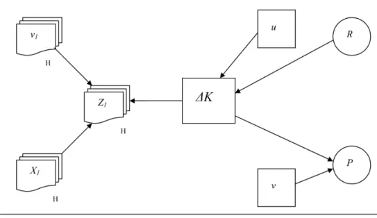
Figure 1 shows that the variable of interest (i.e. ∆K – additions to economically valuable knowledge) is measured inaccurately if one takes either patent statistics P or R&D expenditure R on their own as a measure of innovative output. In this study, we use Principal Component Analysis to create a summary ‘innovativeness’ variable that extracts the common variance from both R&D and patent statistics (levels and stocks) whilst discarding the irrelevant variance that includes noise, measurement error and idiosyncratic variation.1 _In

addition, we restrict our analysis to four ‘complex technology’ sectors (Cohen et al., 2000) that are known for their intense R&D and patenting activity. By concentrating on these hand-picked sectors, we aim to get the best possible observations on firm-level innovation.

1_{For a more detailed discussion of how to measure firm-level innovative activity, and the advantages of}

Figure 1: The Knowledge ‘Production Function’: A Simplified Path Analysis Diagram (based

on Griliches 1990:1671)

3

Database Description and Summary Statistics

This paper uses an original database that we created by matching the NBER patent database with the Compustat file database.2 _{The patent data has been obtained from the NBER Database (Hall et al. 2001b).}

The NBER database comprises detailed information on almost 3 416 957 U.S. utility patents in the USPTOs TAF database granted during the period 1963 to December 2002.

The initial sample of firms was obtained from the well-known Compustat 3 _{database for the ‘complex}

technology’ sectors. These firms were then matched with the firm data files from the NBER patent database and we found all the firms4_{that have patents. The final sample thus contains both patenters and non-patenters.} 2_{We would like to thank Bronwyn Hall for providing us with her calculations of Tobin’s q for the Compustat}

data used in this paper.

3_{Compustat has the largest set of fundamental and market data representing 90% of the worlds market}

capitalization. Use of this database could indicate that we have oversampled the Fortune 500 firms. Being included in the Compustat database means that the number of shareholders in the firm was large enough for the firm to command sufficient investor interest to be followed by Standard and Poors Compustat, which basically means that the firm is required to file 10-Ks to the Securities and Exchange Commission on a regular basis. It does not necessarily mean that the firm has gone through an IPO. Most of them are listed on NASDAQ or the NYSE.

4_{The patent ownership information reflects ownership at the time of patent grant and does not include}

subsequent changes in ownership. Also attempts have been made to combine data based on subsidiary re-lationships. However, where possible, spelling variations and variations based on name changes have been merged into a single name. While every effort is made to accurately identify all organizational entities and report data by a single organizational name, achievement of a totally clean record is not expected, particularly in view of the many variations which may occur in corporate identifications. Also, the NBER database does not cumulatively assign the patents obtained by the subsudiaries to the parents, and we have taken this limi-tation into account and have subsequently tried to cumulate the patents obtained by the subsidiaries towards the patent count of the parent. Thus we have attempted to create an original database that gives complete firm-level patent information.

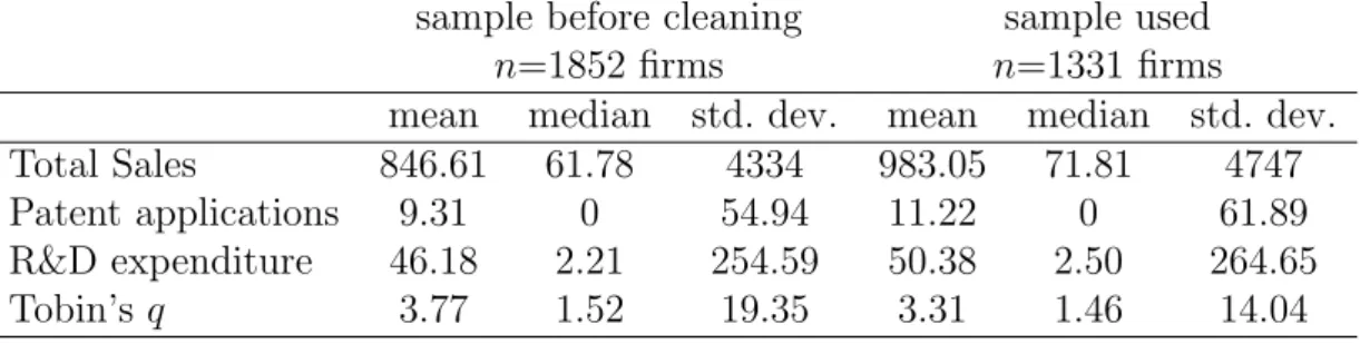
Table 1: Summary statistics before and after data-cleaning, SIC’s 35-38

sample before cleaning

sample used

n=1852 firms

n=1331 firms

mean

median std. dev.

mean

median std. dev.

Total Sales

846.61

61.78

4334

983.05

71.81

4747

Patent applications

9.31

0

54.94

11.22

0

61.89

R&D expenditure

46.18

2.21

254.59

50.38

2.50

264.65

Tobin’s q

3.77

1.52

19.35

3.31

1.46

14.04

Table 2: The Distribution of Firms by Total Patents, 1963-1999 (SIC’s 35-38)

0 or more 1 or more 10 or more 25 or more 100 or more 250 or more 1000 or more

Firms 1331 877 614 457 229 131 57

Descriptive statistics of the sample before and after cleaning are shown in Table 1. Initially using the Compustat database, we obtain a total of 1852 firms which belong to the SICs 35-38 and this sample consists of both patenting and non-patenting firms. These firms were then matched to the NBER database. After this initial match, we further matched the year-wise firm data to the year-wise patents applied by the respective firms (in the case of patenting firms) and finally, we excluded firms that had less than 7 consecutive years of good data. Thus, we have an unbalanced panel of 1331 firms belonging to 4 different sectors. Since we intend to take into account sectoral effects of innovation, we will proceed on a sector by sector basis, to have (ideally) 4 comparable results for 4 different sectors. The two digit SIC codes that we use are SIC 35 (industrial and commercial machinery and computer equipment), SIC 36 (electronic and other electrical equipment and components, except computer equipment), SIC 37 (transportation equipment) and SIC 38 (measuring, analyzing and controlling instruments; photographic, medical and optical goods; watches and clocks).

We find that 34% of the firms in our sample have no patents. Thus the intersection of the two datasets gave us 877 patenting firms who had taken out at least one patent between 1963 and 1999, and 454 firms that had no patents during this period. (See Table 2 for more details on the distribution of firms by total patents.) The total number of patents taken out by this group over the entire period was 291 555, where the entire period for the NBER database represented years 1963 to 2000, and we have used 217 770 of these patents in our analysis i.e. representing about 75% of the total patents ever taken out at the US Patent Office by the firms in our sample. Figure 2 shows the the number of patents per year for our database, for each of the four sectors.

Though the NBER database provides the data on patents applied for from 1963 till 2000, it contains information only on the granted patents and hence we might see some bias towards the firms that have applied in the end period covered by the database due the lags faced between application and the grant of the patents.

Table 3: Contemporaneous correlations

be-tween Patents and R&D expenditure

SIC 35 SIC 36 SIC 37 SIC 38

CORRELATIONS ρ 0.5281 0.3834 0.4475 0.7766 p-value 0.0000 0.0000 0.0000 0.0000 RANK CORRELATIONS ρ 0.4227 0.4672 0.4574 0.4587 p-value 0.0000 0.0000 0.0000 0.0000 Obs. 5986 6219 1972 5241

Table 4: Contemporaneous correlations

be-tween patents/sales and R&D/sales

SIC 35 SIC 36 SIC 37 SIC 38

CORRELATIONS ρ 0.3446 0.3297 0.0900 0.3230 p-value 0.0000 0.0000 0.0001 0.0000 RANK CORRELATIONS ρ 0.0851 0.2153 0.2322 0.1336 p-value 0.0000 0.0000 0.0000 0.0000 Obs. 5986 6219 1972 5241

0 1000 2000 3000 4000 5000 6000 7000 8000 1960 1965 1970 1975 1980 1985 1990 1995 2000 2005 No. Patents Year SIC 35 SIC 36 SIC 37 SIC 38

Figure 2: Number of patents per year. SIC 35: Machinery & Computer Equipment, SIC

36: Electric/Electronic Equipment, SIC 37: Transportation Equipment, SIC 38: Measuring

Instruments.

Hence to avoid this truncation bias (on the right) we consider the patents only till 1999 so as to account for the average 3-year gap between application and grant of the patent.5 _{Table 3 shows that patent numbers are}

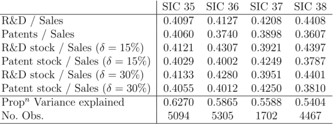
well correlated with (deflated) R&D expenditure, albeit without controlling for firm size. To take this into account, Table 4 reports the correlations between firm-level patent intensity and R&D intensity (conventional correlations and also rank correlations that are more robust to extreme observations). For each of the sectors we observe positive and highly significant rank correlations, which nonetheless take values of 0.23 or lower. These results would thus appear to be consistent with the idea that, even within industries, patent and R&D statistics do contain large amounts of idiosyncratic variance and that either of these variables taken individually would be a rather noisy proxy for innovativeness. Indeed, these two variables are quite different not only in terms of statistical properties (patent statistics are much more skewed and less persistent than R&D statistics) but also in terms of economic significance. However, they both yield valuable information on firm-level innovation. As a result, we use Principal Component Analysis to create a composite summary index of firm-level innovative activity. Our synthetic innovativeness index is created by extracting the common variance from a series of related variables: both patent intensity and R&D intensity at time t, and also the actualized 3-year stocks of patents and R&D. These stock variables are calculated using the conventional amortizement rate of 15%, and also at the rate of 30% since we suspect that the 15% rate may be too low (Hall and Oriani 2006). Information on the factor loadings is shown in Table 5. We consider the summary innovativeness variable to be a satisfactory indicator of firm-level innovativeness because it loads well with each of the variables and explains between 54% to 63% of the total variance. An advantage of this composite index is that a lot of information on a firm’s innovative activity can be summarized into one variable (this will be especially useful in the following graphs). A disadvantage is that the units have no ready interpretation (unlike ‘one patent’ or ‘$1 million of R&D expenditure’). In this study, however, we are less concerned with the quantitative point estimates than with the qualitative variation in the importance of innovation over the conditional distribution of Tobin’s q (i.e. the ‘shape’ of the graphs).

5_{This average gap has been referred to by many authors, among others Bloom and Van Reenen (2002) who}

mention a lag of two years between application and grant, and Hall et al. (2001a) who state that 95% of the patents that are eventually granted are granted within 3 years of application.

Table 5: Extracting the ‘innovativeness’ index used for the quantile regressions - Principal

Component Analysis results (first component only, unrotated)

SIC 35 SIC 36 SIC 37 SIC 38

R&D / Sales

0.4097

0.4127

0.4208

0.4408

Patents / Sales

0.4060

0.3740

0.3898

0.3607

R&D stock / Sales (δ = 15%)

0.4121

0.4307

0.3921

0.4397

Patent stock / Sales (δ = 15%)

0.4029

0.4002

0.4249

0.3787

R&D stock / Sales (δ = 30%)

0.4133

0.4280

0.3951

0.4401

Patent stock / Sales (δ = 30%)

0.4055

0.4012

0.4250

0.3810

Prop

_{Variance explained}

_0.6270

_0.5865

_0.5588

_0.5404

No. Obs.

5094

5305

1702

4467

4

Quantile Regression

We begin this section with a brief introduction to quantile regression, and then apply it to our dataset.

4.1

An Introduction to Quantile Regression

Standard least squares regression techniques provide summary point estimates that calculate the average effect of the independent variables on the ‘average firm’. However, this focus on the average firm may hide important features of the underlying relationship. As Mosteller and Tukey explain in an oft-cited passage:

“What the regression curve does is give a grand summary for the averages of the distributions corresponding to the set of x’s. We could go further and compute several regression curves corresponding to the various percentage points of the distributions and thus get a more complete picture of the set. Ordinarily this is not done, and so regression often gives a rather incomplete picture. Just as the mean gives an incomplete picture of a single distribution, so the regression curve gives a correspondingly incomplete picture for a set of distributions”

(Mosteller and Tukey 1977:266).

Quantile regression techniques can therefore help us obtain a more complete picture of the underlying relationship between innovation and firm performance. In our case, estimation of linear models by quantile regression may be preferable to the usual regression methods for a number of reasons. First of all, we know that the standard least-squares assumption of normally distributed errors does not hold for our database because the values for Tobin’s q follow a skewed distribution (see the evidence in Table 1). Whilst the optimal properties of standard regression estimators are not robust to modest departures from normality, quantile regression results are characteristically robust to outliers and heavy-tailed distributions. In fact, the quantile regression solution ˆβθ is invariant to outliers of the dependent variable that tend to ± ∞ (Buchinsky 1994). Another

advantage is that, while conventional regressions focus on the mean, quantile regressions are able to describe the entire conditional distribution of the dependent variable. In the context of this study, high-q firms are of interest in their own right, we don’t want to dismiss them as outliers, but on the contrary we believe it would be worthwhile to study them in detail. This can be done by calculating coefficient estimates at various quantiles of the conditional distribution. Finally, a quantile regression approach avoids the restrictive assumption that the error terms are identically distributed at all points of the conditional distribution. Relaxing this assumption allows us to acknowledge firm heterogeneity and consider the possibility that estimated slope parameters vary at different quantiles of the conditional distribution of Tobin’s q.

The quantile regression model, first introduced by Koenker and Bassett (1978), can be written as:

yit= x0itβθ+ uθit with Quantθ(yit|xit) = x0itβθ (1)

where yitis the growth rate, x is a vector of regressors, β is the vector of parameters to be estimated, and

u is a vector of residuals. Qθ(yit|xit) denotes the θth conditional quantile of yit given xit. The θthregression

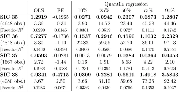
Table 6: Quantile regression estimation of equation (4): the coefficient and t-statistic on

‘in-novativeness’ reported for the 10%, 25%, 50%, 75% and 90% quantiles. Coefficients significant

at the 5% level appear in bold.

Quantile regression

OLS

FE

10%

25%

50%

75%

90%

SIC 35

1.2919 -0.1965 0.0271 0.0942 0.2307 0.6873 1.2807

(4648 obs.)

3.36

-0.34

3.93

14.72

23.40

45.58

44.46

SIC 36

0.7277 -0.1736 0.1537 0.2946 0.4590 1.1032 2.2329

(4848 obs.)

3.30

-1.10

22.83

59.56

52.70

86.01

97.13

SIC 37

0.0593 -0.0281

0.0013

0.0079

0.0384 0.0364 0.0453

(1567 obs.)

2.72

-1.44

0.16

0.91

5.53

4.22

2.10

SIC 38

0.9341 0.4715 0.0309 0.2281 0.6619 1.4918 3.5843

(4080 obs.)

3.67

2.50

3.66

31.10

59.68

73.26

92.42

where ρθ(.), which is known as the ‘check function’, is defined as:

ρθ(uθit) =

½

θuθit if uθit≥ 0

(θ − 1)uθit if uθit< 0

¾

(3) In other words, we estimate the regression coefficients at different quantiles by attributing different weights to datapoints, depending on whether they are above or below the ‘line of best fit’. This contrasts with standard regression estimators that implicitly give equal weights to points on either side of the regression line.

Equation (2) is then solved by linear programming methods. As one increases θ continuously from 0 to 1, one traces the entire conditional distribution of y, conditional on x (Buchinsky 1998). More on quantile regression techniques can be found in the surveys by Buchinsky (1998) and Koenker and Hallock (2001); for applications see Buchinsky (1994), Mata and Machado (1996), Coad (2006) and also the special issue of

Empirical Economics (Vol. 26 (3), 2001).

4.2

Quantile regression results

In keeping with the literature,6_{we estimate the following linear regression model:}

qi,t= α + β1IN Ni,t−1+ β3SIZEi,t−1+ β4IN Di,t+ yt+ ²i,t (4)

where qit, the dependent variable, is the value of Tobin’s q for firm i at time t. IN N represents the

‘innovativeness’ index, and the control variables are lagged size (measured in sales (deflated dollars)) and 3-digit industry dummies. We also control for common macroeconomic shocks by including year dummies (yt).

The numerical results for OLS, fixed-effects and quantile regression estimation are reported in Table 6. OLS regressions estimate a positive and significant influence of innovative activity on Tobin’s q, for each of the four sectors. Fixed-effects regressions, on the other hand, only detect a significant (positive) influence for SIC

6_{See, among others, Griliches (1981), Pakes (1985), Jaffe (1986), Cockburn and Griliches (1988), Hall}

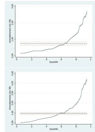
0.00 0.50 1.00 1.50 2.00 2.50 innovativeness (sic 35) 0 .2 .4 .6 .8 1 Quantile 0.00 1.00 2.00 3.00 innovativeness (sic 36) 0 .2 .4 .6 .8 1 Quantile −0.05 0.00 0.05 0.10 0.15 innovativeness (sic 37) 0 .2 .4 .6 .8 1 Quantile 0.00 1.00 2.00 3.00 4.00 5.00 innovativeness (sic 38) 0 .2 .4 .6 .8 1 Quantile

Figure 3: Variation in the ‘innovativeness’ coefficient (β

from Equation (4)) over the

condi-tional quantiles. Confidence intervals extend to 95% confidence intervals in either direction.

Horizontal lines represent OLS estimates with 95% confidence intervals. SIC 35: Machinery

& Computer Equipment (top left), SIC 36: Electric/Electronic Equipment (top right), SIC

37: Transportation Equipment (bottom left), SIC 38: Measuring Instruments (bottom right).

Graphs made using the ‘grqreg’ Stata module (Azevedo 2004).

38.7 _{Median (50%) quantile regression results, which correspond to the Minimum Absolute Deviation (MAD)}

estimator, are significantly lower than the OLS estimates for each of the four sectors. This suggests that the OLS estimates, which are not robust to extreme observations or non-gaussian distributions of residuals, may be biased upwards.

The quantile regression results are always positive and mostly statistically significant. The quantile re-gression coefficients can be interpreted as the partial derivative of the conditional quantile of y with respect to particular regressors, δQθ(yit|xit)/δx. Put differently, the derivative is interpreted as the marginal change

in y at the θth _{conditional quantile due to marginal change in a particular regressor (Yasar et al. 2006). For}

each of the four sectors, the coefficient on innovativeness is much larger at the higher quantiles. The coefficient estimates at the 75% quantiles are over three times bigger than those at the 25% quantiles, for each of the four sectors. Values for the pseudo-R2 _{also rise as we move to the upper quantiles.}

Figure 3 allows a visual appreciation of the quantile regression results. All four of the sectors show a common pattern, although the plot for SIC 37 is much less elegant than for the other sectors (this is in part due to the smaller number of observations, and perhaps also due to the peculiarities of this sector8_{). At the}

lowest quantiles of the conditional Tobin’s q distribution, the coefficients on innovativeness are very low, close to zero, which suggests that these firms’ efforts at innovation are barely recognized by the stock market. As we move up the conditional distribution, however, the coefficient rises significantly, especially at the extreme upper quantiles. For those firms with the highest values of Tobin’s q, additional efforts at innovation result in relatively large gains in market value. It is plain to see that the OLS point estimates, shown here as horizontal lines with 95% confidence intervals, provide limited information on the relationship between innovation and market value.

Our results appear to be quite robust, not only across the four ‘complex technology’ sectors, but also using different data. We repeated the analysis using either 3-year R&D stocks or 3-year patent stocks (instead of combining them in a composite index) and we obtained qualitatively similar results. Furthermore, we repeated the analysis using the Hall et al. (2005) database,9 _{and obtained similar results (although with fewer}

observations).

5

Conclusion

Previous research using conventional regression estimators shows that the stock market does recognize inno-vative activity undertaken by firms. These studies find a positive and significant influence of R&D or patents on market value. However, quantile regression analysis adds a new dimension to the literature and suggests that the influence of innovation on market value varies dramatically across the (conditional) market value distribution. For firms with a low value of Tobin’s q, the stock market will barely recognize their attempts to innovate. For firms with the highest values of Tobin’s q, however, their market value is particularly sensitive to innovative activity. Innovative efforts by these firms, measured in terms of R&D expenditure or patenting activity, are particularly highly valued.

If firms are lucky, their stock market value will soar, and a major determinant of their resulting performance will be their successful efforts at innovation. However, other firms may also direct a lot of resources to innovative activity, and unless they ‘get lucky’ and come up with an innovation, these resources will be wasted, with little to show for them. Our results therefore emphasize the fundamentally uncertain nature of innovation and technological progress.

Many years ago, John Keynes wrote: “If human nature felt no temptation to take a chance, no satisfaction (profit apart) in constructing a factory, a railway, a mine or a farm, there might not be much investment merely as a result of cold calculation” (1936:150) – the same is certainly true for investment in R&D. Need it be reminded, an innovation strategy is even more uncertain than playing a lottery, because it is a ‘game of chance’ in which neither the probability of winning nor the prize can be known for sure in advance. In the face of such radical uncertainty, some firms may well be overoptimistic (or indeed risk-averse) about what

7_{See Hall et al. (2005:26) for a discussion of the poor performance of the fixed-effect estimator in this}

particular case.

8_{SIC 37 (Transportation Equipment) contains manufacturing sectors as diverse as ship-building, bicycles,}

and guided missiles. Furthermore, whilst the other 3 sectors are bona fide ‘high-tech’ sectors, many subclasses of SIC 37 have rather more mature technological bases. For an amusing anecdote on the diversity of industries grouped together in the ‘Transportation Equipment’ class, see Griliches (1990:1667).

9_{This database is publicly available (subject to conditions) from Bronwyn Hall’s website:}

they will actually gain. For other firms, there may be over-investment in R&D because of the ‘managerial prestige’ attached to having an over-sized R&D department. As a result, we cannot rule out the possibility that many firms invest in R&D far from something which could correspond to the ‘profit-maximizing’ level (whatever ‘profit-maximizing’ may mean). In fact, we remain pessimistic that R&D will ever enter into the domain of ‘rational’ decision-making (i.e. a ‘cost-benefit analysis’). Successful innovation, and the ‘super-star’ performance that may result, require risk-taking and perhaps just a little bit of craziness.

References

Azevedo, J.P.W. (2004) “grqreg: Stata module to graph the coefficients of a quantile regression” Boston College Department of Economics.

Bloom, N., and J. Van Reenen (2002) “Patents, Real Options and Firm Performance” Economic Journal 112, C97-C116.

Buchinsky, M. (1994) “Changes in the U.S. Wage Structure 1963-1987: Application of Quantile Regression”

Econometrica 62, 405-458.

Buchinsky, M. (1998) “Recent Advances in Quantile Regression Models: A Practical Guide for Empirical Research” Journal of Human Resources 33 (1), 88-126.

Cefis, E. and L. Orsenigo (2001) “The persistence of innovative activities: A cross-countries and cross-sectors comparative analysis” Research Policy 30, 1139-1158.

Chan, L.K.C., Lakonishok, J., and T. Sougiannis (2001) “The Stock Market Valuation of Research and Devel-opment Expenditures” Journal of Finance 56 (6), 2431-2456.

Coad, A. (2006) “Understanding the Processes of Firm Growth – a Closer Look at Serial Growth Rate Cor-relation” Cahiers de la Maison des Sciences Economiques No. 06051 (S´erie Rouge), Universit´e Paris 1 Panth´eon-Sorbonne, France.

Coad, A., and R. Rao (2006) “Innovation and Firm Growth in ‘Complex Technology’ Sectors: A Quantile Regression Approach” Cahiers de la Maison des Sciences Economiques No. 06050 (S´erie Rouge), Universit´e Paris 1 Panth´eon-Sorbonne, France.

Cockburn, I., and Z. Griliches (1988) “Industry Effects and Appropriability Measures in the Stock Market’s Valuation of R&D and Patents” American Economic Review Papers and Proceedings 78 (2), 419-423. Cohen, W.M., Nelson, R.R., and J.P. Walsh (2000) “Protecting their intellectual assets: Appropriability

conditions and why US manufacturing firms patent (or not)” NBER working paper 7552.

Dosi, G. (1988) “Sources, Procedures, and Microeconomic Effects of Innovation” Journal of Economic

Liter-ature 26 (3), 1120-1171.

Griliches, Z. (1981) “Market Value, R&D, and Patents” Economics Letters 7, 183-187.

Griliches, Z. (1990) “Patent Statistics as Economic Indicators: A Survey” Journal of Economic Literature 28, 1661-1707.

Hall, B.H. (1993a) “The Stock Market Valuation of R&D Investment during the 1980s” American Economic

Review Papers and Proceedings 83 (2), 259-264.

Hall, B.H. (1993b) “Industrial Research During the 1980s: Did the Rate of Return Fall?” Brookings Papers

on Economic Activity (Microeconomics), 289-344.

Hall, B.H., Jaffe, A., and M. Trajtenberg (2001a) “Market Value and Patent Citations: A First Look” Paper E01-304, University of California, Berkeley.

Hall, B.H., Jaffe, A., and M. Trajtenberg (2001b) “The NBER Patent Citation Data File: Lessons, Insights and Methodological Tools” NBER Working Paper 8498.

Hall, B.H., Jaffe, A., and M. Trajtenberg (2005) “Market Value and Patent Citations” Rand Journal of

Economics 36 (1), 16-38.

Hall, B.H., and R. Oriani (2006) “Does the market value R&D investment by European firms? Evidence from a panel of manufacturing firms in France, Germany, and Italy” International Journal of Industrial

Jaffe, A.B. (1986) “Technological Opportunity and Spillovers of R&D: Evidence from Firms’ Patents, Profits, and Market Value” American Economic Review 76, 984-1001.

Keynes, J.M. (1936) The general theory of employment, interest, and money, MacMillan, London. Koenker, R., and G. Bassett (1978) “Regression Quantiles” Econometrica 46, 33-50.

Koenker, R., and K.F. Hallock (2001) “Quantile Regression” Journal of Economic Perspectives 15 (4), 143-156. Mata, J., and J.A.F. Machado (1996) “Firm Start-up Size: A Conditional Quantile Approach” European

Economic Review 40, 1305-1323.

Mosteller, F., and J. Tukey (1977) Data Analysis and Regression Addison-Wesley, Reading, MA.

Pakes, A. (1985) “On Patents, R&D, and the Stock Market Rate of Return” Journal of Political Economy 93, 390-409.

Yasar, M., Nelson, C.H., and R.M. Rejesus (2006) “Productivity and Exporting Status of Manufacturing Firms: Evidence from Quantile Regressions” Weltwirtschaftliches Archiv, in press.