HAL Id: hal-01233712
https://hal.archives-ouvertes.fr/hal-01233712
Submitted on 25 Nov 2015
HAL is a multi-disciplinary open access
archive for the deposit and dissemination of
sci-entific research documents, whether they are
pub-lished or not. The documents may come from
teaching and research institutions in France or
abroad, or from public or private research centers.
L’archive ouverte pluridisciplinaire HAL, est
destinée au dépôt et à la diffusion de documents
scientifiques de niveau recherche, publiés ou non,
émanant des établissements d’enseignement et de
recherche français ou étrangers, des laboratoires
publics ou privés.
Active polarimetric imaging with adaptive contrast
optimization (Orale)
François Goudail, Matthieu Boffety, Nicolas Vannier, Nicolas Bertaux,
Frédéric Galland, Patrick Feneyrou
To cite this version:
François Goudail, Matthieu Boffety, Nicolas Vannier, Nicolas Bertaux, Frédéric Galland, et al.. Active
polarimetric imaging with adaptive contrast optimization (Orale). 6th International Symposium on
optronics in defence and security (OPTRO 2014), Jan 2014, Paris, France. �hal-01233712�
Active polarimetric imaging with adaptive contrast optimization
François Goudail1, Matthieu Boffety1, Nicolas Vannier1, Nicolas Bertaux2, Frédéric Galland2, Patrick
Feneyrou3
1Laboratoire Charles Fabry, Institut d’Optique, RD 128, 91127 Palaiseau, France.Email:
2Institut Fresnel, Marseille, France.Email: [email protected]
3Thales research and Technology - France, RD128, 91767 Palaiseau Cedex, France.Email:
ABSTRACT
We propose a method for semi-automatic target de-tection and contrast optimization making joint use of an adaptive polarimetric imager and a statistical image segmentation algorithm. It can be used to de-tect targets that differ from the background by their polarimetric properties. This method illustrates the benefits of integrating digital processing algorithms in the image acquisition process, rather than using them only for post-processing.
1 INTRODUCTION
Active polarimetric imaging is a powerful tool for re-vealing contrasts that do not appear in standard in-tensity images and has been proven useful in such domains as remote sensing, biomedical imaging or industrial inspection [1, 2]. Extensive research has been conducted for optimizing the characteristics of the systems, in particular to maximize the contrast between the object of interest and the background in target detection applications [3, 4, 5, 6, 7]. Most of these studies assumed that the polarimetric proper-ties (i.e., the Mueller matrices) of the objects in the scene were known beforehand. This is obviously a limitation to their practical use. We propose in this paper a solution to this issue that consists in per-forming iteratively image segmentation and contrast optimization. It is based on the iterative operation of an active polarimetric imager whose illumination and analysis polarization states can be anywhere on the Poincaré sphere, and of a fast and unsupervised image segmentation algorithm. The benefits of this approach are demonstrated on real-world images in difficult situations where target and background dif-fer only by polarimetric properties.
The paper is organized as follows. In Section 2, we describe the principle of an adaptive polarimetric imager and in Section 3, the principle of polarimet-ric contrast optimization is reviewed. In Section 4, we present a contrast optimization method that can be applied to a scene whose polarimetric properties are unknown, and its validation on images from a
laboratory polarimetric imager. We draw some con-clusions and perspectives in Section 5.
2 CONTRAST OPTIMIZATION IN
POLARIMET-RIC IMAGING
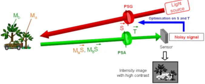
The principle of an adaptive polarimetric imager is illustrated in Fig. 1.
Figure 1: Principle of an adaptive scalar polarimetric imaging. PSG: Polarization State Generator. PSA: Polarization State Ana-lyzer.
The system illuminates the scene with light com-ing from a thermal or laser source. Polarization state in illumination is defined by a Stokes vector Sgenerated thanks to a Polarization State Genera-tor (PSG). In the practical implementation we use, the PSG is composed of two Liquid Crystal Vari-able Retarders and one polarizer [8]. The output beam allows illuminating the scene uniformly in po-larization and intensity. The polarimetric properties of a region of the scene corresponding to a pixel in the image is characterized by its Mueller matrix M. The Stokes vector of the light scattered by this region is S0 = MS. It is analyzed by a
Polariza-tion State Analyser (PSA), which is a generalized polarizer whose eigenstate is the Stokes vector T.
As for the PSG, in the experimental setup we use, the PSA is composed of two Liquid Crystal Variable Retarders and one polarizer.
The number of photoelectrons measured at a pixel of the sensor is:
i =ηI0 2 T
TM
where the superscript T denotes matrix
transposi-tion. In this equation, S and T are unit intensity, purely polarized Stokes vectors, I0 is a number of
photons and η is the conversion efficiency between photons and electrons.
3 CONTRAST OPTIMIZATION IN THE
PRES-ENCE OF SPATIAL FLUCTUATIONS
The system represented in Fig. 1 can be used to op-timize the contrast in the acquired intensity image. Let us assume that the scene is composed of two re-gions: a target characterized by an average Mueller matrix < Ma >and a background characterized by
an average Mueller matrix < Mb >. The objective
is to determine the configurations of the PSG and the PSA so that the contrast between these to re-gions in the final intensity image is maximize. The appropriate expression of the contrast, that is, the function to optimize, depends on the type of noise that affects the scene. Different cases have been analyzed: additive Gaussian noise [6], Poisson shot noise and speckle noise [9], spatial fluctuations of the polarization properties [7].
In this paper, we will consider that the image is disturbed by two different types of noise: The first one is additive sensor noise which will be assumed of zero mean and variance σ2. The second one is
due to the fact that from one pixel to the next, the Mueller matrix randomly fluctuates around its aver-age value. Each pixel belonging to region u ∈ {a, b} has a Mueller matrix M that deviates from the av-erage matrix < Mu > of this region. These
spa-tial fluctuations are characterized by their correlation matrices defined as:
Gu=< (VM− V<Mu>)(VM− V<Mu>)T > (2)
with VMthe 16-component vector obtained by
read-ing the Mueller matrix M in the lexicographic order. Using this notation and taking into account additive noise, Eq. 1 can be written as:
i = ηI0
2 [T ⊗ S]
TV
M + n (3)
where ⊗ denotes the Kronecker product and n is a random variable of zero mean and variance σ2.
No-tice that i is now a random variable whose statistical properties depend on the region where the pixel is located. If we assume that the fluctuations of VM
and n are independent, the mean and variance of i in region u ∈ {a, b} are given by [7]:
< i >u = ηI0/2 × [T ⊗ S]TV<Mu> (4)
var[i]u = (ηI0/2)2× [T ⊗ S]TGu[T ⊗ S] + σ2(5)
Our objective is to optimize the discrimination between the target and the background region in the intensity image. To quantifiy the quality of this dis-crimination, we will use the Fisher ratio [10]. Using the notation defined above, it is defined as:
F (S, T) = [< i >a− < i >b]
2
var[i]a+ var[i]b
(6) By using Eqs 3, 4 and 5, it can be put in the following form: F (S, T) = [T ⊗ S] TG target[T ⊗ S] [T ⊗ S]TG f luct[T ⊗ S] + 8/SN R (7) where Gf luct = Ga + Gb is the average
covari-ance matrix of the Mueller matrix fluctuations over the scene, Gtarget = (< Ma > − < Mb >)(<
Ma > − < Mb >)T is the interclass covariance
matrix, which represents the difference between the average Mueller matrices of the two regions, and SN R = (η2I2
0)/σ2 is the signal to noise ratio due
to the presence of additive noise.
To optimize the image, one has to determine the optimal couple of illumination and analysis states (S,T) that maximizes the function F (S, T) defined
in Eq. 7. It has been shown that this method is effi-cient and can for example reveal objects appearing through diffusive media [7]. However, it is based on the hypothesis that the statistics of the Mueller ma-trices in the target and in the background regions are known. In the following section, we propose a method to deal with cases where this knowledge is not available.
4 ADAPTIVE POLARIMETRIC CONTRAST
OP-TIMIZATION
4.1
Principle of the method
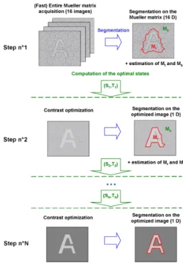
The proposed method is illustrated on Fig.2. The first step consists in acquiring the full Mueller image with a global integration time of t0 seconds. The
in-tegration time of each images is thus about t0/16,
and they consequently have a low SNR. We then use a fast and unsupervised segmentation algo-rithm adapted to such noisy 16-dimensional images (described below) that gives a first estimation of the target shape. Due to low SNR and inhomogeneities in some components, this shape estimation is not perfect. However, from this first segmentation it is possible to estimate the polarimetric properties of the pixels inside and outside the segmented region (object and background). One estimates the aver-age Mueller matrix
Mu= 1 NΩu X k∈Ωu Muk (8)
with u = {in, out} corresponding to pixels inside or outside the segmentation boundaries, Ωuthe set
containing the NΩu pixels in the region u, and M
k u
the Mueller matrix of the pixel k in the region u. The spatial fluctuations are characterized by the covari-ance matrix given by:
Gu= 1 NΩu X k∈Ωu [VMk u − VMu][VMuk− VMu] T (9)
withVM the vectorized Mueller matrix M .
Figure 2: Different steps to detect and recognize a target from a background
Using these estimates, the PSG and PSA states S1and T1that maximize the contrast between the
two regions are determined by optimizing the cri-terion in Eq. 7. These states are implemented on the imaging system to acquire a single image with an integration time equal to t0 and thus a better
SNR. This image is then segmented in order to re-fine the shape of the target, which allows one to obtain a better estimation of the polarimetric prop-erties of the target and the background (Mu, Gu)
(u ∈ {in, out}), and thus a better estimation of the optimal PSG/PSA states S2 and T2. These new
states can be implemented on the imaging system to acquire a new image, that is segmented to further refine the PSG/PSA estimation. This process of ac-quisition / segmentation / contrast optimization can be iterated until the contrast between the target and the background is sufficient. The number of itera-tions will depend on the complexity of the scene and
on the difference of polarimetric properties between the target and the background. However, since all the steps but the first one are based on single im-age acquisitions, it is robust to object movements in the scene.
4.2
Segmentation algorithm
One of the key elements of this method is the segmentation algorithm. It should be fast, require no intervention from the user, and be adapted to both 1D and 16D noisy intensity images. We thus use the polygonal active contour (snake) proposed in [11, 12], initially developed for 1D images and that has been generalized to multi-dimensional im-ages. This algorithm relies on a Minimum De-scription Length (MDL) criterion, based on a non-parametric description of the gray level fluctuations that are modeled with K-bin histograms. Both the number and location of the nodes of the polygonal contour used to separate the object from the back-ground are estimated iteratively via the optimization of the MDL criterion which does not contain any pa-rameter to be tuned by the user.
The most time-consuming step in this algorithm is the calculus of the K statistics needed to update the height of the K bins of the histogram after each deformation of the contour [12]. Fast computation of these statistics are obtained with summing K pre-computed images along the contour of the objet, and a number of bins K between 8 to 16 usually yields a good tradeoff between computation time and discrimination capability. The computation time of this operation can be significantly reduced by vec-torizing it with the streaming single instruction mul-tiple data (SIMD) extensions (SSE). As described in [12], for images with a pixel number N ≤ 32767, it allows computing S = 8 statistics simultaneously with only one SSE summation. Assuming that the grey level values of the 16 Muller matrix components are independent, the generalization of the 1D MDL criterion to 16D is straightforward [11], the data ad-equacy term in the MDL criterion being simply the sum of the data adequacy terms for each of the 16 components. It is thus necessary to calculate 16 K statistics, which implies k SSE summations, where k is the smallest integer not less than (16 K)/S. Since in the considered images N ≤ 32767, S = 8 and thus only k = 2 K SSE summations are necessary, allowing to keep a reduced computation time even when dealing with 16D intensity images. For exam-ple a 152×162 pixel image is segmented with K=8 in 4 milliseconds for 1D images and less than 20 mil-liseconds for 16D images on a 2.5 GHz processor laptop.
4.3
Experimental validation
In order to validate this method, we have used the adaptive polarimetric imager described in Section 2. The scheme of the observed scene is represented in Fig. 3.a. The target is composed of metallic adhe-sive tape and the background of white plastic. Both are placed behind a piece of diffusing paper, they cannot be discriminated on a standard intensity im-age (see Fig. 3.b).
(a) (b)
Figure 3:(a) Scheme of the scene. (b) Intensity image.
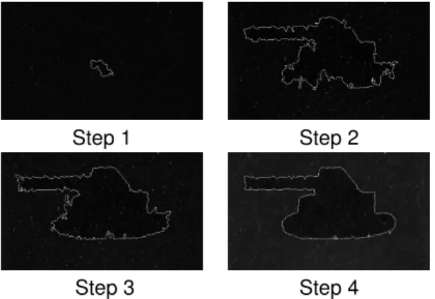
Step 1 Step 2
Step 3 Step 4
Figure 4: Segmentation and contrast optimization on scene of Fig. 3 in 4 iterations
We first acquire full Mueller data with a short in-tegration time and we apply the 16D segmentation algorithm to extract a first estimated shape of the target (see Fig. 4, step 1). The segmented shape corresponds to a small part of the object, due to the presence of noise and spatial fluctuations of the polarimetric properties in the scene. We extract the polarimetric properties of the regions inside and outside this approximate contour, and compute the PSG/PSA states maximizing the contrast criterion in Eq. 7. By implementing these polarization states on the imaging system, we acquire the image pre-sented in Fig. 4 (step 2). In this optimized intensity image, the quality of the segmentation and the con-trast between the target and the background have been significantly improved. Using this image for a new 1D segmentation step, we obtain an
improve-ment of the shape estimation. However, as some fluctuations remain in the images, the shape esti-mation has still some defects. Two further iterations of the same process yield the image in Fig.4 (step 4), where we observe that the contrast is sufficiently improved to yield a precise estimation of the object shape. In this case, a correct shape estimation is finally recovered in 4 iterations
5 Conclusion
Polarimetric techniques have a large potential to im-prove the performance of imaging systems. One of their main advantages is to reveal contrasts that do not appear in classical images, which is of great terest in defence but also in medical imaging or in-dustrial inspection. We have presented a method-ology for automatic target detection based on the it-erative interplay between an active polarimetric im-ager with adaptive capabilities and a snake-based image segmentation algorithm. Its efficiency has been demonstrated in a difficult situation where the target and the background had the same intensity reflectivities and differed only by their polarimetric properties.
This method does not require prior knowledge of the polarimetric properties of the scene, and pro-vides a scalar image with optimal contrast that can be further exploited by a human observer. These re-sults illustrate the benefits of integrating digital pro-cessing algorithms in the image acquisition process, rather than using them only for post-processing. Further research is necessary to precisely quantify the benefits of this method, in terms of acquisition time and robustness to target motion during acqui-sition. We are currently investigating these issues.
References
[1] J. S. Tyo, M. P. Rowe, E. N. Pugh, and N. En-gheta, “Target detection in optical scattering media by polarization-difference imaging,” Ap-plied Optics35(11), 1855–1870 (1996).
[2] J. E. Solomon, “Polarization imaging,” Applied Optics20(9), 1537–1544 (1981).
[3] A. B. Kostinski and W. M. Boerner, “On the polarimetric contrast optimization,” IEEE Trans. Antennas Propagat.35, 988–991 (1987).
[4] A. B. Kostinski, B. D. James, and W. M. Boerner, “Optimal polarization of partially po-larized waves,” J. Opt. Soc. Am. A5(5), 58–64
[5] M. Richert, X. Orlik, and A. De Martino, “Adapted polarization state contrast image,” Opt. Express17, 14,199–14,210 (2009).
[6] F. Goudail and A. Bénière, “Optimization of the contrast in polarimetric scalar images,” Opt. Lett.34, 1471–1473 (2009).
[7] G. Anna, F. Goudail, and D. Dolfi, “Polarimet-ric target detection in the presence of spatially fluctuating Mueller matrices,” Optics Letters36,
4590–4592 (2011).
[8] G. Anna, H. Sauer, F. Goudail, and D. Dolfi, “Fully tunable active polarization imager for contrast enhancement and partial polarimetry,” Appl. Opt.51, 5302–5309 (2012).
[9] G. Anna, F. Goudail, P. Chavel, and D. Dolfi, “On the influence of noise statistics on po-larimetric contrast optimization,” Appl. Opt.51,
1178–1187 (2012).
[10] K. Fukunaga, Introduction to statistical pattern recognition (Academic Press, San Diego, 1990).
[11] F. Galland and P. Réfrégier, “Minimal stochas-tic complexity snake-based technique adapted to unknown noise model,” Opt. Lett. 30(17),
2239–2241 (2005).
[12] N. Bertaux, F. Galland, and P. Réfrégier, “Multi-initialisation segmentation with non-parametric minimum description length snake,” Electronics Letters47(10), 594–595 (2011).