HAL Id: hal-03191499
https://hal.univ-reunion.fr/hal-03191499
Submitted on 7 Apr 2021HAL is a multi-disciplinary open access archive for the deposit and dissemination of sci-entific research documents, whether they are pub-lished or not. The documents may come from teaching and research institutions in France or abroad, or from public or private research centers.
L’archive ouverte pluridisciplinaire HAL, est destinée au dépôt et à la diffusion de documents scientifiques de niveau recherche, publiés ou non, émanant des établissements d’enseignement et de recherche français ou étrangers, des laboratoires publics ou privés.
Spain
María A. García-Valiñas, Fernando Arbués, Inmaculada Villanúa
To cite this version:
María A. García-Valiñas, Fernando Arbués, Inmaculada Villanúa. Is industrial water used effi-ciently? A case study in Spain. Journal of Cleaner Production, Elsevier, 2019, 229, pp.931-940. �10.1016/j.jclepro.2019.04.368�. �hal-03191499�
IS INDUSTRIAL WATER USED EFFICIENTLY? A CASE STUDY IN SPAIN
Mª Ángeles García-Valiñas (corresponding author) Oviedo Efficiency Group
Department of Economics University of Oviedo Avda. del Cristo s/n 33006 Oviedo (Spain) e-mail: [email protected] Fernando Arbués
Aragon Public Economics Research Group Institute of Environmental Science (IUCA) University of Zaragoza
Violante de Hungría 23 50009 Zaragoza (Spain) e-mail: [email protected] Inmaculada Villanúa
Aragon Growth, Demand and Natural Resources Research Group University of Zaragoza
Gran Vía, 2
50005 Zaragoza (Spain) e-mail: [email protected]
1.- Introduction
Several European Union institutions have highlighted the importance of assessing efficiency in the use of water in all sectors (EC, 2012). In recent years, water drawn from the public water supply for use in industry has accounted for between 2% and 50% of total use for all economic activities in European Union (EU) countries (EUROSTAT, 2014). Self-supplied water and water from other sources for industrial use represents over 60 % of this total use, with this figure reaching as high as 90% in some countries (EUROSTAT, 2014). Moreover, industrial activity is considered one of the worst polluters of water bodies (AMEC, 2014).
As a consequence, a comprehensive evaluation of industrial water use becomes a key issue. On the one hand, industries can probably reduce water consumption and achieve significant water savings—an especially valuable option in a context of scarcity-. On the other hand, pollution abatement is an additional aim when improving water management in the industrial sector. Pollutant emissions might be reduced, leading to a cleaner environment and water bodies. These aims related to water consumption and reducing pollution could be achieved through both the adoption of pro-environmental
organizational systems and/or investment in green technologies. In any case, both aims are significant when assessing the efficiency of water use from an integrated perspective.
This paper is focused on the environmental efficiency of water use in a sample of Spanish industries in Zaragoza. This city lies in the Ebro river basin, which is Spain’s largest river basin, covering 85,660 km2. Public authorities have traditionally faced certain difficulties when managing water bodies. On the one hand, this area has suffered from severe water stress in recent years, with the water exploitation index reaching levels higher than 40% (EEA, 2018). On the other hand, the Ebro river basin has always experienced poor natural water quality due to its chemical composition. Moreover, the agricultural and urban wastewater discharges into the river have worsened the situation (de Marcos, 2016). On top of that, Zaragoza is the biggest city in the Ebro river basin, and an area of fairly intensive industrial activity (INE 2017a, 2017b). Consequently, industrial water pollution and water consumption are significant issues that must be addressed.
From a methodological point of view, the efficiency in the use of industrial water has been assessed by means of Data Envelopment Analysis (DEA) techniques (Cooper et al., 2007), in particular, through the use of directional distance functions (Chambers et al., 1998) adapted to this specific scenario. This methodology proposes jointly modelling inputs, desirable and undesirable outputs by identifying the maximum attainable expansion of desirable outputs in one specific direction and the largest feasible contraction of inputs and undesirable outputs in another specific direction. The use of directional functions is considered a flexible technique that is perfectly suited to the economic problem examined in this research. The findings will be very useful when it comes to designing future public policies related to water efficiency in the industrial sector.
The paper is structured as follows. The literature review section summarizes the main contributions to the literature in this field. Section 3 provides a detailed explanation of the method applied to evaluate the environmental efficiency of water use. The contextual framework, the variables and the data set are described in Section 4, while Section 5 presents the main results and empirical findings. Finally, Section 6 concludes with a summary of the main results, including a discussion about some policy implications and future extensions of this research.
2.- Literature review
Although there are plenty of studies assessing the efficiency of water services (Abbott et al., 2012; D’Inverno et al., 2017; Dong et al. 2018; Gémar et al., 2018; Suárez-Varela et al., 2017), papers analysing the eco-efficiency of water use in the industrial sector are relatively scarce in the literature. The eco-efficiency concept refers to create more value with less environmental impact. In 1992, the World Business Council for Sustainable Development (WBCSD) indicated that: “eco-efficiency is achieved by the delivery of competitively-priced goods and services that satisfy human needs and bring quality of life, while progressively reducing ecological impacts and resource intensity throughout the life-cycle to a level at least in line with the Earth’s estimated carrying capacity.” (WBCSD, 2000; p.9).
Water resource eco-efficiency has been analysed at different scales. In this respect, we find studies at a national (Chen and Jia, 2017; Hu et al., 2006; Wang et al., 2018; You and An, 2016; Zhang et al., 2008) or regional scale (Charmondusit et al., 2016; Deng et al., 2016; Yang and Zhang, 2018), or even at the level of specific economic sectors. Regarding the latter, water use efficiency has been assessed in both agricultural (among others, Beltrán-Esteve, 2013; Huang, 2005; Speelman et al., 2008; Ullah et al., 2016) and industrial activities (Fan et al., 2017; Jiang et al., 2016; Karel and Charmondusit, 2008; Skouteris et al., 2018; Zhou et al., 2017). However, the number of papers focused on the environmental efficiency of water use in the agricultural sector far outnumbers the studies focused on industrial water use efficiency.
When measuring the eco-efficiency of water resources at the industrial sector, most of empirical studies have applied any of the following methodologies: 1) the ratio approach (Charmondusit and Keartpakpraek, 2011; Ingaramo et al., 2009; Kharel and Charmondusit, 2008; Skouteris et al., 2018; Zhou et al., 2017); 2) Life Cycle Assessment (LCA) methods1 (Angelis-Dimakis et al., 2016; Georgopoulou et al., 2017; Maxime et al., 2006; Wigger et al., 2017); and 3) the frontier approach, based on parametric Stochastic Frontier Analysis (SFA) (Atkinson and Halabí, 2005; Lei and Huang, 2015) or
non-
1 Some studies (Wang et al., 2015; Zhang et al., 2008) have recommended combining DEA and LCA
methods. LCA methodology requires the creation of an inventory of flows entering and leaving the production system for each activity. The application of this kind of methodologies would require detailed information related to water quality when finishing the production process (before being discharged) and the quality of water finally discharged. Thus LCA method requires detailed information on the concentration of aimed pollutant substances. In our case, since we are using a micro-data set of manufacturing firms located in the same geographical area, it has not been possible to get individual and detailed information on the concentrations of pollutant substances over an extended period of time. This shortage makes not possible to apply that specific methodological approach.
parametric DEA (Fan et al., 2017; Hu et al., 2006; Jiang et al., 2016; Wang et al., 2015; Wang et al., 2018; Yang and Zhang, 2018; You and An, 2016; Zhang et al., 2008).
At present, most researchers use different DEA models to evaluate water use efficiency at national or regional level. For example, Hu et al. (2006) analyse water use efficiency in China at the country level under a conventional DEA framework. Nevertheless, their approach only measures economic efficiency and does not account for the fact that industrial activities produce both desirable and undesirable outputs (e.g. pollution). Hence, many researchers have improved DEA models by incorporating both desirable and undesirable outputs in efficiency analyses. In this respect, Generalized DEA (GDEA) methodology is a popular approach (Fan et al., 2017; Zhang et al., 2008; Wang et al., 2015; Jiang et al., 2016; Yu et al., 2017). Only a few papers have considered the use of directional distance functions (Wang et al., 2018; Yang and Zhang, 2018).
Regarding the output variables, whereas the desirable output is represented through more standard indices like industrial value-added (Zhang et al. 2008; Yu et al., 2016), or industrial Gross Domestic Product (Wang et al., 2015; Jiang et al., 2016; You and An, 2016; Fan et al., 2017; Yang and Zhang, 2018; Wang et al. 2018), there is more heterogeneity when it comes to define environmental pollutants. Most studies include more than one undesirable dimension. In this respect, the most popular parameters are Chemical Oxygen Demand (COD) emissions (Zhang et al., 2008; Wang et al., 2015; Yu et al., 2016; Fan et al., 2017), Ammonia Nitrogen (NH4–N) discharges (Wang et al., 2015; Yu et al., 2016; Wang et al., 2018), Suspended Solid (SS) waste (Zhang et al., 2008; Fan et al., 2017; Yang and Zhang, 2018) or Sulphur Dioxide (SO2) emissions (Zhang et al., 2008; Fan et al., 2017; Yang and Zhang, 2018). Other variables, such as dust or soot emissions are less frequently used (Zhang et al., 2008; Jiang et al., 2016; Yang and Zhang, 2018). With regard to input variables, water consumption is systematically included in all the studies assessing the industrial water use efficiency.
Although results are heterogeneous, it is possible to detect some common findings. First of all, a positive relationship between development and eco-efficiency has been detected. Then, the most developed areas exhibit the better performance levels (Chen and Yia, 2017; Deng et al., 2016; Yang and Zang, 2018; You and An, 2016; Zhang et al., 2008). Closely connected to the previous issue, it has been remarked the role of technology, with a positive impact on water use efficiency (Li and Ma, 2015; Wang et al., 2015; Yang and Zang, 2018; You and An, 2016; Zhang et al., 2017). Furthermore Deng et
al. (2016) indicates that higher dependence on foreign trade leads to improve water use efficiency.
Additionally, it has been found that institutional factors are significant key-drivers of water use efficiency. Higher levels of efficiency have been detected in those areas with stringent regulations linked to water quality (Li and Ma, 2015; Wang et al., 2018; You and An, 2016). Moreover, water pricing (level and structure issues) could lead to get strong improvements in water use efficiency (Chen and Jia, 2017; Wang et al., 2018; You and An, 2016; Zhan et al., 2008).
Regarding pollutant substances, Yu et al. (2016) find that COD emissions are still the main driver of inefficiency in the pulp and paper industry. Wang et al. (2015) indicate that the inefficiency of industrial sector in Chinese regions is mainly generated by pollutants' abatement performance as shown by potentials reduction of COD and NH4– N. Fan et al. (2017) conclude that SO2 emissions are the limiting factor for eco-industrial development. Moreover, they show that there is great potential for water and energy conservation in industrial parks in China.
Finally, all of the studies focused on industrial water efficiency have been developed on the base of aggregated data (provincial, regional or national). The most disaggregated view is adopted by Fan et al. (2017), who analyse the eco-efficiency level in 40 industrial parks in China. Although an overwhelming majority of them have assessed water use efficiency considering the global industry sector, a few of them have analysed specific industrial activities. This is the case of Yu et al. (2016) who assess the eco-efficiency of the pulp and paper industry—a major polluter—in 16 Chinese provinces. Definitively, all previous studies have used aggregated data rather than micro databases where the observational unit is the firm. In this paper, we use a different approach based on individual information related to a sample of manufacturing industries. Moreover, a temporal dimension is considered in the analysis, which allows us to assess the impact of public policies.
3.- Methodological issues
The methodological approach adopted in this research extends the metafrontier approach (O’Donnell et al., 2008) to measure technological differences in the management of particular inputs and/or outputs with the integration of environmental aspects when assessing productive efficiency.This is an approach used in several recent
empirical papers as Beltrán-Esteve (2013), Beltrán-Esteve et al. (2014), Picazo-Tadeo et al. (2014) or Suárez-Varela et al. (2017).
3.1. Distance functions. Managerial and technical efficiency
Let us suppose that there are k = 1…K production units that use a set of N inputs x = (xf, xv), where xf denotes the fixed input and xv a bundle of variable inputs used to obtain the vector of outputs Y =(y, b). The output vector includes a set of M desirable outputs and J undesirable outputs, y and b, respectively. The metatechnology is represented by a set that contains all achievable combinations of variable inputs xv that, given an amount of fixed input xf, allow obtain a level of good output y, and generate a bad output b. It is formally defined as:
L (xf, y, b) = [xv| (x, y, b) ∈ T] (1)
T denotes all technologically feasible combinations of inputs and outputs. It is assumed that the metatechnology satisfies the standard properties that Shephard (1970) suggests. Additionally, we assume weak disposability of undesirable outputs, b, which means that a simultaneous reduction of good and bad outputs is feasible, but the isolated disposal of bad outputs may not be possible (Färe et al, 1989). Moreover, we adopt the hypothesis of null-joint production, so good and bad outputs are jointly produced (Shephard and Färe, 1974). These methodological assumptions are frequently used in the literature when modelling the performance of pollution-generating technologies (Dakpo et al., 2016). When there are undesirable outputs, the directional metadistance function (Färe and Grosskopf, 2000) is as follows:
"# = %&, (, ); + = ,−+./, +0, −+123
= 456[8|(&/− 8+./)]=> ?&@, ,( + 8+02, () − 8+1)B (2) where g=(-gxv, gy, -gb) denotes the so-called direction vector. The function in (2) has a lower bound of zero (Chambers et al., 1998), and models inputs and outputs trying to find the maximum achievable expansion of outputs in the gy direction and the largest possible contraction of variable inputs and bad outputs in the –gxv and –gb directions, respectively. Moreover, the directional metadistance function is a versatile tool for assessing efficiency as it allows approaching the technological frontier by means of
alternative methods focused on different performance frameworks (Suárez-Varela et al., 2017).
As a consequence, this methodology is especially useful when analysing the use of specific inputs or outputs. In this case, it would be interesting to assess firms’ water use efficiency by focusing, on the one hand, on water consumption, and on the other hand, on water pollution. In other words, the aim here is to examine a potential reduction of variable input i (water consumption) and the bad output (water pollution), while maintaining the other inputs and outputs, i.e., to assess technical efficiency in the management of water. In this context, the directional metadistance function becomes: "#D = 〈&, (, ); + = %,−&
/F, 0/HF2, 0, −)3〉
= 456%8D|,(1 − 8D)&/F, &/HF23=>%&@, (, (1 − 8D))3 (3) The directional distance functions can also be determined regarding the
technology of different industry sectors. Accordingly, the technology of sector h is made up only of observations of production units within this group, and can also be denoted by the short-run input requirement set defined as:
Lh (xf, y, b) = [xv| (x, y, b) ∈ Th] (4) with Th representing all the combinations of inputs and outputs achievable by producers in sector h. Formally, the directional distance functions computed with regard to the technology of sector h (composed of Kh operational units) in the integrated management of water use (w) are :
4#D = 〈&, (, ); + = %,−&
/F, 0/HF2, 0, −)3〉 = 456%KD |,(1 − K
D )&/F, &/HF23=>L%&@, (, (1 − KD))3 (5) So directional distance functions linked to the technology of sector h will always
be equal to or lower than directional metadistance functions computed with regard to the metatechnology. Figure 1 presents an intuitive approach to the analytical framework described above. Water technology includes two dimensions, the input xvw, (water consumption) and the negative output b (water pollution). Note that only two dimensions are represented. In this context, we are interested in optimizing the use of water and reducing water pollution. In short, we aim to minimize the damage to water
bodies. The technology is graphically represented under the assumption of weak disposability.
[FIGURE 1]
The operational units of two industrial sectors (1, 2) are denoted by crosses (x) and dots () respectively. A joint frontier or metafrontier is built by enveloping the units of both sectors (dotted grey line). However, it is also possible to build a specific frontier for each sector, in order to assess their managerial performance. The upper dashed line corresponds to the Sector 1 frontier, while the solid line represents the Sector 2 frontier. Also note that the frontier functions in Figure 1 have a vertical and parallel section to the ordinate axis to allow the possibility to exclusively reduce input xvw. Assume that we want to assess the performance of an inefficient operational unit in Sector 1, which is circled in Figure 1. It is considered inefficient because it is responsible for higher levels of consumption and generates higher levels of water pollution than other units lying on the frontier. Other firms are able to obtain the same level of output as the unit evaluated, ceteris paribus the remaining inputs.
By projecting the inefficient unit to the metafrontier (the distance from the unit to point A in Figure 1), we can assess the global technical efficiency of that unit. In other words, our reference group is composed of all the observations in the industry, without distinguishing between sectors. Nevertheless, two units in different sectors are not directly comparable through this distance measure (Suárez-Varela et al., 2017). The technical efficiency index breakdown into two components (managerial efficiency and the metatechnology ratio) has a more straightforward reading, as shown as follows.
With managerial efficiency (the distance from the unit to point B in Figure 1) we match the inefficient unit with other units in the same sector. By comparing similar firms, e.g., two paper-producing firms, the performance assessment complies with an important requirement for applying non-parametric techniques, namely the need for relatively homogeneous units (Hwang et al., 2016). By establishing different manufacturing groups, we reduce the heterogeneity of the units analysed.
Additionally, the sector efficiency measured though the metatechnology ratio is based on the distance between the specific sector frontier and the joint frontier (which includes all the sectors in the sample). This gap, which shows technological differences between the two sectors, represents how far each sector is from global water use efficiency. Analytically, we use the directional distance/metadistance functions
presented in Section 3.1 to calculate the metatechnology ratios proposed by O’Donnell et al. (2008). Specifically, the metatechnology ratio (MR) of sector h for a global water performance assessment w can be defined as:
"MDL〈&, (, ); +
D= %,−&/F, 02, 0, −)3〉 = NOPℎRSPTU OVVSPSORP(D⁄NOPℎRSPTU OVVSPSORP(DL = (1 − 8D) (1 − K⁄ D ) (6)
Note that the metatechnology ratio is calculated using technical efficiency scores with an upper bound of one –which indicates full efficiency. Moreover, efficiency scores computed considering the technology of sector h will be equal to or higher than those related to the metatechnology. In line with O’Donnell et al. (2008), our approach gives a satisfactory decomposition of technical efficiency assessed with regard to the metafrontier, into the product of technical efficiency evaluated with regard to the frontier of sector h and the metatechnology ratio for sector h (which evaluates the distance between the technology of this sector to the joint technology). Moreover, this procedure permits the decomposition of technical efficiency into managerial efficiency, which assesses the performance of decision units in the sample as contrasted to top performance in their group, and sector efficiency, which measures the nearness of the technology of sector h to the joint technology.
3.2. Two-step empirical approach
The empirical approach proposed in this research has been structured in two steps. First of all, efficiency indices have been calculated using directional metadistance/distance functions. These functions have been computed using Data Envelopment Analysis (DEA) techniques. Details on DEA programs could be checked in the Appendix. Additionally, variable returns to scale (VRS) are assumed. However, Chen and Ang (2016) show that simply adding a convexity constraint to the constant return to scale (CRS) model with weak disposability would not necessarily mean that the new model is one with VRS technology with weak disposability (Färe and Grosskopf, 2003). The right VRS formulation under the weak disposability hypothesis was first shown by Shephard (1970), who developed a highly non-linear model. Kuosmanen (2005) and Kuosmanen and Podinovski (2009) extended Shephard’s VRS model by designing a convex and fully linearizable model. In this research, the linearization proposed in Kuosmanen (2005) and Kuosmanen and Podinovski (2009) is applied to calculate efficiency indices.
Next, a second step is applied to identify key drivers of efficiency. This second stage could provide some insights to guide public policies related to water use in the manufacturing sector. The equation to be estimated is the following:
KDX = V,YX, Z[, \X2 (7) Managerial efficiency could be explained by firms’ specific factors (sk), temporal factors (rt) and subsector dummies (dk). To empirically estimate equation (7), we use Simar and Wilson’s (2007) contribution to analyse managerial efficiency scores obtained through DEA techniques. Their methodological approach allows us to account for the nature of our DEA-based scores of efficiency and their serial correlation. Basically, it involves simulating a sensible data-generating process, by means of artificial bootstrap samples from this process, and computing standard errors and confidence intervals for the parameters of interest (Simar and Wilson, 2007).
4.- Data set
The sample considered in this research includes 60 firms in Zaragoza’s manufacturing industry over the period 2004-2007. Since it is a short period of time, we evaluate the performance under the assumption that there is no technological change. Database elaboration is an important contribution of this research, since it is the first applied study considering a micro-database in this field. As specified hereafter, it includes information taken from different sources, related to water use and production process.
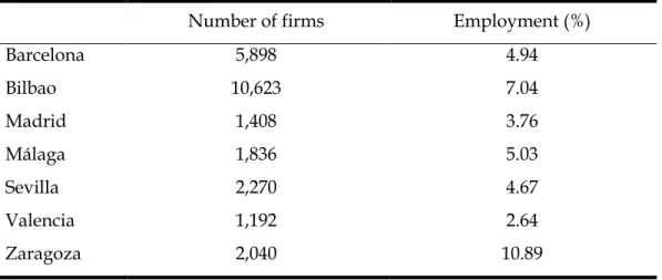
Zaragoza is located in the central area of the Ebro River Basin in North-Eastern Spain (South-Western Europe). It is the fifth largest city in Spain with 666,938 inhabitants (INE, 2017c). Water management in the city is based on an in-house provision framework. A non-outsourced public organization is providing supply and sewerage water services in the city. Moreover, Zaragoza is an important industrial core (Arbués et al., 2010), with 2,040 companies registered in the city council in 2015 (INE, 2017b). Table 1 displays some economic indices revealing the weight of industrial activities in Zaragoza.
In terms of the number of industrial companies, Zaragoza ranks fourth, very close to the third-ranked city (Valencia). Looking at the proportion of employment in the industrial sector, Zaragoza has the highest rate (10.89%), far above other big cities such as Valencia (2.64%), Madrid (3.76%) or Bilbao (7.04%).
The panel database is not balanced, and it includes production data for different manufacturing activities in Zaragoza. Activities are classified according to the NACE Rev.2 (Statistical classification of economic activities in the European Community), using a 4-digit code. Manufacturing firms have been split into three sectors. Sector 1 (SEC1) includes processed food and chemical activities, comprising 22 firms and 82 observations. Sector 2 (SEC2) is related to metal manufacturing activities, including 22 firms and 79 observations. Finally, Sector 3 (SEC3) covers electrical equipment and furniture manufacturing, with 16 firms and 59 observations2.
Since we have access to the specific activity of each manufacturing firm, we built the data base controlling that the kind of activities included in each NACE Rev 2 4-digit code are developing homogeneous activities (i.e., in the paper industry, no recycled-paper producers are included). Moreover, when clustering the activities we considered some aspects linked to the final use of water3. In this respect, Sector 1 is including manufacturing activities where water is an essential component of their products. The majority of companies in Sector 2 use water mainly for cleaning their installations. Finally, firms in Sector 3 basically consider sanitary and cooling uses.
Six variables are used to characterize the production set. Regarding the output variables, both the economic activity and water pollution have been considered. On the one hand, firms’ net sales (NSAL) is the variable representing the firms’ good output. The information on net sales is taken from the SABI database4.
On the other hand, a water pollution index (F) is considered as a negative output. This index is calculated by the Zaragoza city council, and it indicates the quality of water
2 The main activities included in Sector 1 comprise food and beverage manufacturing and the
manufacture of paper and chemical products. Sector 2 includes manufacturing activities related to metal and metallic components (steel, metal smelting, metalworking, metallic products). Finally, Sector 3 is basically comprised of the manufacture of electrical and transport equipment, machinery and furniture.
3 The information related to industrial water uses is taken from a survey conducted by the
Zaragoza City Council in 2004. In particular, companies were asked whether they use water for product elaboration, cleaning, cooling and/or sanitary needs of their workers.
4 SABI is a broad database including balance sheet analysis of more than two million Spanish
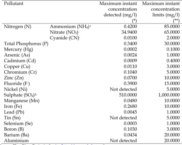
emissions. It is based on the concentration of pollutants per volume of water discharged, with respect to the average values of residential water users. The main parameters considered in the formula are the Suspended Solid (SS) waste and the Chemical Oxygen Demand (COD)5. Wastewater quality controls carried out by the Ebro River Basin Authority6 and the Zaragoza City Council indicate that the majority of reported and controlled pollutants are Chemical Oxygen Demand (COD) and Suspended Solid (SS) waste. Consequently, available data strongly suggest that the use of the index F (based on the most frequent pollutants detected) is fairly well reflecting the industrial wastewater quality in Zaragoza. Moreover, Zaragoza City Council indicates that 33 firms (out of 64) in the sample treat water before discharging it into the public network. Three procedures are detected: sewage, decantation, and separation, being sewage the most frequent treatment (22 firms have their own wastewater treatment plant). Although some direct discharges are observed in some industrial states, none of the firms included in this sample is discharging wastewater directly to water bodies.
Moreover, four input variables have been defined. Labour (L) is measured in terms of the number of workers. The value of the firm’s assets (K) represents the capital of the company. Capital comprises the structural firms’ assets. That is, the assets which are consumed in more than one economic period. The assets’ value is calculated discounting the accumulated depreciation. Both tangible and intangible assets are included.
Water consumption is considered as an additional input (WATER), and includes water drawn from both the municipal network and wells. Finally, the remaining operating expenses (excluding water and labour expenses) are aggregated in a global index (OPEX). Data for all the input variables except water consumption have been taken from the abovementioned SABI database, while the municipal water department has provided information about industrial water consumption.
Regarding the key drivers of efficiency, three main variables have been defined. First of all, the percentage of water taken from wells (PWELL) is included. This source of water is not as closely controlled as the water taken from the municipal network, so the related levels of water efficiency could be lower. However, in general well water quality is
5 The formula applied to calculate the pollution index is the following: F= 0.6* COD/700 + 0.4 *
SS/250. Both parameters are expressed in mg/l.
6 In this respect, the Ebro River Basin Authority ensures periodic water quality controls. This
monitoring activity is carried out before applying any wastewater treatment at the municipal sewage treatment plant. Ebro River Basin monitoring results (check Appendix B) show that the presence of heavy metals or other toxic substances in the wastewater is not significant.
lower when being closer to surface. As a consequence, firms need to abstract water from deeper levels. Thus, energy costs necessary to extract water from wells could emerge as a strong incentive for an efficient water use.
Two additional dummy variables are built. The first one takes a value of 1 when the firm is located in an industrial estate, and 0 otherwise (POL). Such a location generates agglomeration economies that could have an impact on efficiency. The second takes a value of 1 for periods starting after 2004, and 0 otherwise (PREFORM). This second dummy variable is capturing the effect of a tariff reform that took place in 2004. The resulting new water tariff was in place from 2005 on. The tariff reform affects both the structure and the level. Before 2005, urban water tariffs consisted of a huge number of fixed and variable charges. Fixed charge depended on the metering size (this dimension experienced more variability in the case of industrial users) and street category, while variable part depended on the level of daily consumption (setting more than 200 different consumption levels and 134 price levels). Thus, clients bore a different two-part tariff depending on their daily consumption, being the variable charge the most complex dimension. In 2004, variable charge ranked between 0.23 (consumption of 0.03 m3/day) and 1.75 (consumption of 135.73 m3/day). Consequently, the result was a complicated structure, which made extremely difficult for customers to have perfect information and knowledge about water prices. In 2005, that complex variable charge was replaced by an increasing two-block structure for industrial users. Moreover, from 2005 onwards, water bill displays sanitation and supply prices in a separate way, being easier for customers to check both concepts. Compared with the previous tariff, this framework was much simpler to retain and understand, adding more transparency to the pricing system. Since the reform involved a significant simplification of the water tariff structure and price increases for some industrial users7, we would expect it affects positively on industrial water use efficiency. Finally, the second-step equation includes dummy variables for each specific economic activity based on the 4-digit NACE Rev.2 code, in order to control for heterogeneity within the sector.
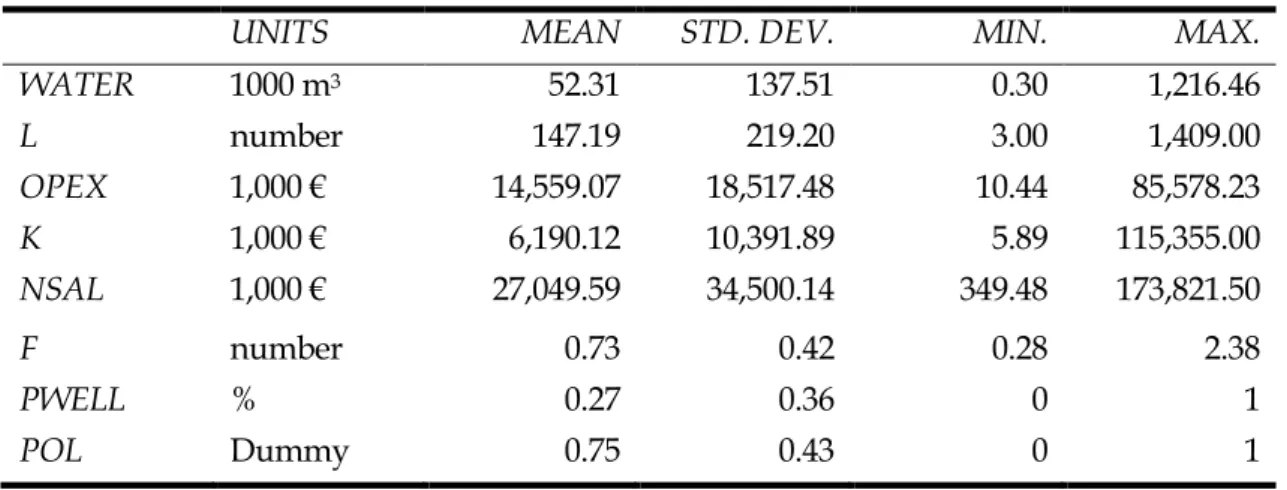
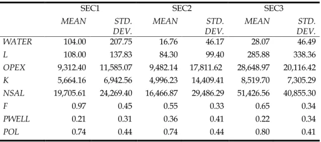
Tables 2 and 3 present the main descriptive statistics. Table 2 includes some descriptive statistics of the whole sample, while Table 3 displays information disaggregated by sector. On average, industrial water consumption per year (WATER) is particularly
7 The reformed tariff lead to average price increases ranked between 12% and 30% for users
consuming less than 30 m3/month. Between that level and 300m3/month, average price increases
were much smaller, and from 400 m3/month, average price experienced decreases between 0.3%
noteworthy, registering a volume of around 52,300 m3. The dispersion in water use is also significant, as clearly shown by the standard deviation and the gap between the minimum and maximum. As expected, dispersion is also observed in other variables that characterize the production process (L, OPEX, K, NSAL). The average value of the pollution index (F) is 0.73, indicating that pollution levels are not high. Actually, this value would not be far from a typical pattern of raw municipal wastewater with minor contributions of industrial wastewater (Henze and Comeau, 2008). Finally, 75% of the firms are located in an industrial estate, and around 27% of industrial water comes from wells.
[TABLE 2]
When looking at specific sectors, we detect some notable differences. As expected, Sector 1 registers the highest levels of water consumption and pollution. By contrast, Sector 2 reports the lowest levels of water use and emissions, with this sector drawing a higher proportion of its water from underground sources. Meanwhile, Sector 3 can be seen as an intensive sector in the use of other inputs (labour, capital, other operational expenses). Regarding the percentage of firms located in industrial estates by sector, no broad gaps are observed between sectors. The highest proportion is found in Sector 3, where 80% of the firms are based in industrial parks.
[TABLE 3]
5.- Results
Efficiency indices have been computed using R software, through the DJL package (Lim, 2018). This package includes various decision support tools based on directional distance functions and DEA (among other techniques). Second-step regression has been carried out using Stata software, through the command simarwilson (Badunenko and Tauchmann, 2018). This command applies the procedure proposed by Simar and Wilson (2007) for regression analysis of DEA efficiency scores.
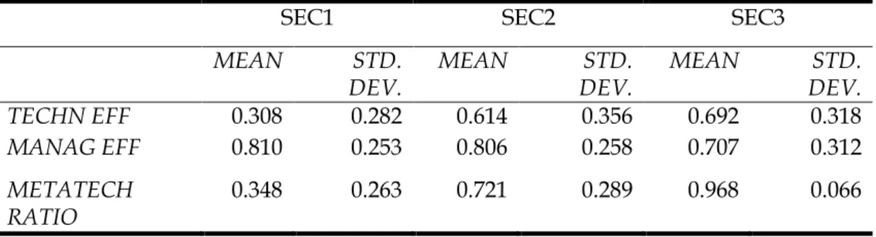
Results are presented in Tables 4 to 6 and Figure 2. Table 4 shows the main efficiency score results by sector. Sector 1 registers the lowest global technical efficiency scores on average, with Sector 3 holding the top position in the ranking.
Metatechnology ratios indicate that Sector 1 has the least environmentally friendly technology in terms of water use. However, after controlling for technological constraints, Sector 1 shows potential reductions in average water use and pollution of around 19%. Sector 3 has the technology that is closest to the joint frontier. With respect to managerial efficiency, it registers potential savings of around 29%. This result is consistent with those obtained in other empirical studies (for example, Zhang et al., 2015 or Wang et al., 2018).
[TABLE 5]
Table 5 displays the results of several tests used to detect statistically significant differences between sectors in terms of efficiency levels. In general, the Kruskal-Wallis test leads us to reject the hypothesis that the sector samples come from the same population. Moreover, when checking differences between pairs, the Wilcoxon test reveals that, in the majority of cases (the null hypothesis is not rejected in the case of the Sector 2 and 3 pair), the samples do not come from populations with the same distribution. Similarly, the Simar-Zelenyuk-Li test (Li, 1996; Simar and Zelenyuk, 2006) results lead us to reject the null hypothesis that the samples have the same probability distribution function, except when comparing Sectors 2 and 3.
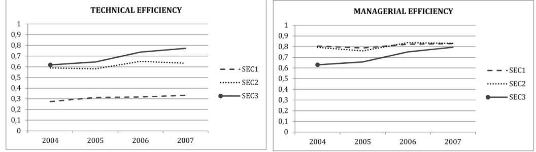
Figure 2 displays the temporal evolution of efficiency indices (technical and managerial) by sectors. Note that, in the case of managerial efficiency, the reference frontier is different for each sector. In general, a rising trend is observed over the period 2004-2007. Both technical and managerial efficiency of electrical equipment and furniture manufacturing activities register the highest increasing rates. Additionally, different patterns are detected. On the one hand, a convergence of the three sectors in terms of managerial efficiency can be observed. However, a slight opposite trend is observed in the case of technical efficiency.
[FIGURE 2]
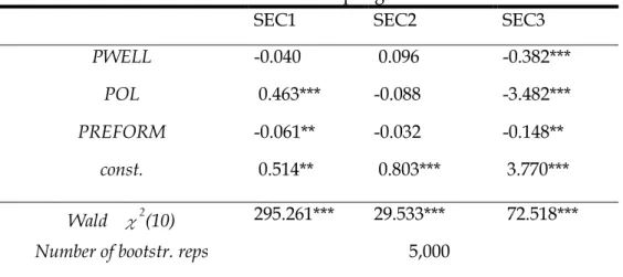
Table 6 shows the second-step regression estimates. The dependent variable is managerial efficiency, expressed in terms of the potential savings in water use and pollution; the higher the values, the lower the efficiency. Heterogeneity is controlled by including subsector
dummies (a dummy variable for each specific activity, excluding one activity in each group). The impact of the three factors differs according to the sector. In Sector 3, for instance, the higher the proportion of water taken from wells, the lower the potential savings; consequently, higher efficiency levels are registered. However, no such effect is detected in Sector 1 or 2.
[TABLE 6]
In line with previous studies such as Li and Ma (2015), You and An (2016) or Wang et al. (2018), among others, price reform has had a positive influence on efficiency in the majority of sectors considered. Thus, potential savings are lower from 2005 onwards. The simplification of the water tariff structure and the increase in the water price level for the majority of users have had a positive impact on managerial efficiency. This result is especially valuable when it comes to designing water price structures. Reducing the complexity of these structures makes it more likely that users will have perfect information about prices and thus helps them to make efficient decisions.
Finally, being located in an industrial area has different impacts depending on the sector. In Sector 1, there is an increase in potential savings, while in Sector 3 the inefficiency levels are reduced. Moreover, industries located in industrial estates and involved in metal manufacturing activities do not experience significant changes in their levels of managerial efficiency. These results could be partially explained by differences in water supply and wastewater management in each industrial estate (a similar result is obtained in Fan et al., 2017). According to the Aragon Institute of Development (IAF, 2018) there are 40 industrial estates in Zaragoza. Regarding water supply, most of these estates (32) are connected to the urban public network. This connection to the public water supply can either be on an individual basis (each firm has its own meter installed and pays the public water supplier directly) or a collective basis (using a collective meter). Conversely, 6 industrial parks are responsible for drawing their own water from underground sources, and 15 manage their own water tanks8. In terms of wastewater, there are also some differences. Wastewater flows are completely discharged to the municipal sewer network in 32 industrial estates. That wastewater is treated in two municipal treatments plants. Additionally, there are 3 industrial parks that manage their own sewage treatment plants, where wastewater is treated before dumping it into the Ebro and Gállego rivers.
8 Water stored in these tanks is used for non-productive activities such as cleaning public areas
Finally, we observe direct discharges in 5 industrial estates. Those differences may well be directly linked to the variety of impacts found in the empirical exercise. In this respect, the small size of the database has prevented us from using a more disaggregated variable to capture the individual industrial estate effects.
6.- Conclusions
The aim of this paper is to analyse the environmental efficiency of water use, using a sample of manufacturing industries located in the urban area of Zaragoza (Spain). To this end, a DEA framework based on directional distance functions is applied. In terms of technical efficiency scores, Sector 1 registers the highest inefficiency levels, while Sector 3 presents the shortest distance to the metafrontier. Those figures could be easily linked to differences in the technology and production process. As we mentioned previously, Sector 2 (metal manufacturing activities) and 3 use water mainly for cleaning or cooling. The margin to reduce water is higher in these sectors, since it is easier to introduce low-consumption technologies. However, Sector 1 comprises activities where water is a key component of their products, while the kind of product conditions the amount of water. Differences in pollution levels are also contributing to increase the gap.
By contrast, when assessing the performance within each technological sector, this gap narrows, with managerial efficiency scores ranging from 0.81 (Sectors 1 and 2) to 0.71 (Sector 3). These results show that the technology in Sector 1 (high levels of water pollution and consumption) is not close to the metafrontier. The metatechnology ratios indicate that the technology in Sector 1 is poor in terms of water management, while the technology in Sector 3 is the closest to the joint frontier. Sector 2 lies in an intermediate position.
Analysing the impact of several factors on managerial efficiency, we also observe significant differences among sectors. First of all, the higher the share of water drawn from wells, the higher the managerial efficiency levels. This effect is exclusively observed in the electrical equipment and furniture manufacturing sector, with no significant impacts detected in the other sectors. Second, water price reform has had a positive and significant effect on managerial efficiency. Reducing the complexity of water price structure and adding more transparency to the billing system have led to improve efficiency in the majority of manufacturing sectors. Third, no clear findings can be drawn about whether or not the firms are located in an industrial park. Being located
in an industrial state is not per se a guarantee of higher efficiency levels in the use of water. The heterogeneity related to water supply and wastewater management in each industrial area could be behind the differences in water efficiency levels. However, due to the limited size of our database, we have not been able to test this hypothesis. In conclusion, the relative influence of the analysed variables on water use efficiency varies notably among sectors.
In the light of the results, it strongly recommended designing a simple water pricing/taxation framework that allows reducing water industrial consumption and internalizing the negative externality caused by polluting water. However, and closely related to this, it is worth noting that not all the pollutant substances demand the same cleaning efforts. Several substances such as heavy metals are extremely dangerous for health and environment, requiring more intensive and expensive treatments. Some industrial activities are characterized by high-level emissions of those dangerous substances, and could generate stronger environmental damages. Public policies should be modulated accordingly.
It is worth noting two limitations of this study that should be addressed in future research. On the one hand, the empirical analysis has been carried out by splitting the sample into three groups. However, a higher level of disaggregation may be desirable when it comes to designing public policies. Thus, an interesting future extension of this research could involve the use of broader micro-data bases. Additionally, extended databases would allow considering other clustering schemes (i.e.: based on the industrial state). On the other hand, this study is focused on a specific city (Zaragoza), and it may well be the case that our findings do not apply to other areas.
Nevertheless, and despite criticism, some of the conclusions linked to the idea of simplicity and transparency as highly desirable features of water prices (OECD, 1987) could be extended to other contexts. In this respect, simpler structures are connected to higher awareness and knowledge level on water tariffs by users, and consequently to higher probability of efficient reactions when price changes. Moreover, more transparency through the price breakdown (supply and sanitation concepts) in the water bill contributes to enrich the information that final users received. Finally, higher transparency and administrative simplicity leads to improve water governance (Silva-Pinto and Cunha-Marques, 2017) and, hence, the efficiency in the water sector.
Acknowledgements
We would like to thank the financial support of the Spanish Ministry of Economy and Competitiveness and the European Regional Development Fund (project with reference ECO2016-75237-R).
References
Abbott, M., Cohen, B., Wang, W.C., 2012. The performance of the urban water and wastewater sectors in Australia. Util. Policy. 20, 52-63. https://doi.org/10.1016/j.jup.2011.11.003
AMEC, 2014. Contribution of Industry on Pollutant Emissions to Air and Water, Report for European Commission (DG Environment). Publications Office of the European Union, Luxemburg.
Angelis-Dimakis, A., Alexandratou, A., Balzarini, A., 2016. Value chain upgrading in a textile dyeing industry. J. Clean. Prod. 138, 237-247. https://doi.org/10.1016/j.jclepro.2016.02.137.
Arbués, F., García-Valiñas, M.A., Villanua, I., 2010. Urban water demand for service and industrial use: The case of Zaragoza. Water Resour. Manag. 24, 4033-4048. https://doi.org/10.1007/s11269-010-9645-5.
Atkinson, S.E., Halabí, C.E., 2005. Economic efficiency and productivity growth in the post-privatization Chilean hydroelectric industry. J. Prod. Anal. 23, 245-273.
https://doi.org/10.1007/s11123-005-1329-4.
Badunenko, O., Tauchmann, H., 2018. Simar and Wilson two-stage efficiency analysis for Stata. FAU Discussion Papers in Economics 08/2018. Friedrich-Alexander Universität Erlangen-Nürnberg Institute for Economics, Erlangen. https://www.econstor.eu/bitstream/10419/179503/1/1023793822.pdf.
(accessed 3 January 2019).
Beltrán-Esteve M., 2013. Assessing technical efficiency in traditional olive grove systems: A directional metadistance function approach. Ec. Agr. Rec. Nat./Agr.
Resour. Ec. 13, 53–76. https://doi.org/10.7201/earn.2013.02.03.
Beltrán-Esteve M., Gómez-Limón J.A., Picazo-Tadeo A.J., Reig-Martínez E., 2014. A metafrontier directional distance function approach to assessing eco-efficiency. J.
Prod. Anal. 41, 69–83. https://doi.org/10.1007/s11123-012-0334-7.
Chambers, R., Chung, Y., Färe R., 1998. Profit, directional distance functions and Nerlovian efficiency. J. Optimiz. Theory App. 98, 351–364. https://doi.org/10.1023/A:1022637501082.
Charmondusit, K., Keartpakpraek, K., 2011. Eco-efficiency evaluation of the petroleum and petrochemical group in the map Ta Phut Industrial Estate, Thailand. J. Clean. Prod. 19, 241-252. https://doi.org/10.1016/j.jclepro.2010.01.013.
Charmondusit, K., Gheewla, S.H., Mungcharoen, T., 2016. Green and sustainable innovation for cleaner production in the Asia-Pacific region. J. Clean. Prod. 134, 443-446. https://doi.org/10.1016/j.jclepro.2016.06.160.
Chen, C., Ang, S., 2016. Measuring environmental efficiency. An application to US electric utilities, in Zhu, J. (Ed.), Data Envelopment Analysis. International Series in Operations Research & Management Science, vol. 238, 345-366. Springer, Boston.
Chen, C., Jia, G., 2017. Environmental efficiency analysis of China's regional industry: a data envelopment analysis (DEA) based approach. J. Clean. Prod. 142, 846-853. https://doi.org/10.1016/j.jclepro.2016.01.045.
Cooper, W.W., Seiford, L.M., Tone, K., 2007. Data Envelopment Analysis. A comprehensive text with models, applications, references and DEA-Solver software. Springer, New York.
Dakpo, K.H., Jeanneaux, P., Latruffe, L., 2016. Modelling pollution-generating technologies in performance benchmarking: Recent developments, limits and future prospects in the nonparametric framework. Eur. J. Oper. Res. 250, 347-359. https://doi.org/10.1016/j.ejor.2015.07.024.
de Marcos, A., 2016. River Basins and Water Management in Spain. Tagus and Ebro River Basin Districts: An Account of their Current Situation and Main Problems. http://www.europarl.europa.eu/RegData/etudes/STUD/2016/536491/IPOL _STU(2016)536491_EN.pdf(accessed 25 June 2018).
Deng, G., Li, L., Song, Y., 2016. Provincial water use efficiency measurement and factor analysis in China: based on SBM-DEA model. Ecol. Indic. 69, 12-18. https://doi.org/10.1016/j.ecolind.2016.03.052.
D’Inverno, G., Carosi, L., Romano, G., Guerrini, A., 2017. Water pollution in wastewater treatment plants: An efficiency analysis with undesirable output. Eur. J. Oper. Res. 269, 24-34. https://doi.org/10.1016/j.ejor.2017.08.028
urban water infrastructure systems in China. J. Clean. Prod. 170, 330-338. https://doi.org/10.1016/j.jclepro.2017.09.048.
EC, 2012. A Blueprint to Safeguard Europe's Water Resources. https://eur-lex.europa.eu/legal-content/EN/TXT/?uri=celex%3A52012DC0673 (accessed 25 June 2018).
EEA, 2018. Use of Freshwater Resources, https://www.eea.europa.eu/data-and-maps/indicators/use-of-freshwater-resources-2/assessment-2 (accessed 25 June 2018).
EUROSTAT, 2014. Water Use in Industry. http://ec.europa.eu/eurostat/statistics-explained/index.php/Archive:Water_use_in_industry. (accessed 25 June 2018). Fan, Y., Bai, B., Qiao, Q, Kang, P., Zhang, Y., Guo, J., 2017. Study on eco-efficiency of
industrial parks in China based on data envelopment analysis. J. Environ.
Manage. 192, 107-115.https://doi.org/10.1016/j.jenvman.2017.01.048.
Färe R., Grosskopf S., 2000. Theory and application of directional distance functions. J.
Prod. Anal. 13, 93–103. https://doi.org/10.1023/A:1007844628920.
Färe, R., Grosskopf, S., Lovell, C.A.K., Pasurka, C., 1989. Multilateral productivity comparisons when some outputs are undesirable: A nonparametric approach.
Rev. Econ. Stat. 71, 90–98.http://dx.doi.org/10.2307/1928055.
Gémar, G., Gómez, T., Molinos-Senante, M., Caballero, R., Sala-Garrido, R., 2018. Assessing changes in eco-productivity of wastewater treatment plants: The role of costs, pollutant removal efficiency, and greenhouse gas emissions. Environ. Impact Assess. 69, 24-31. https://doi.org/10.1016/j.eiar.2017.11.007.
Henze, M., Comeau, Y., 2008. Wastewater characterization, in Henze, M., van Loosdrecht, M.C.M., Ekama, G.A., Brdjanovic, D. (Eds.), Biological Wastewater Treatment. Principles, Modelling and Design, 33-52. IWA Publishing, London. Hu, J.L., Wang, S.C., Yeh, F.Y., 2006. Total-factor water efficiency of regions in China.
Resour. Policy. 31, 217-230. https://doi.org/10.1016/j.resourpol.2007.02.001. Huang, Y., Chen, L., Fu, B., Huang, Z., Gong, J., 2005. The wheat yields and water-use
efficiency in the Loess Plateau: straw mulch and irrigation effects. Agr. Water Manage. 72, 209-222. https://doi.org/10.1016/j.agwat.2004.09.012.
Hwang, S.N., Lee, H.S., Zhu, J. (Eds.), 2016. Handbook of Operations Analytics Using Data Envelopment Analysis. Springer, New York.
IAF, 2018. Suelo Industrial en Aragón, https://www.iaf.es/poligonos/(accessed 15 March 2019).
http://www.ine.es/jaxiT3/Tabla.htm?t=10849(accessed 25 June 2018).
INE, 2017b. Statistical Use of the Central Business Register. http://www.ine.es/dyngs/INEbase/es/operacion.htm?c=Estadistica_C&cid= 1254736160707&menu=ultiDatos&idp=1254735576550 (accessed 25 June 2018). INE, 2017c. Official population figures from Spanish municipalities: Revision of the
Municipal Register.
http://www.ine.es/dynt3/inebase/en/index.htm?padre=527(accessed 25 June 2018).
Ingaramo, A., Heluane, H., Colombo, M., Cesca, M., 2009. Water and wastewater eco-efficiency indicators for the sugar cane industry. J. Clean. Prod. 17, 487-495. https://doi.org/10.1016/j.jclepro.2008.08.018.
Jiang, L., Folmer, H., Bu, M., 2016. Interaction between output efficiency and environmental efficiency: evidence fronm the textile industry in Jiangsu
Province, China. J. Clean. Prod. 113, 123-132.
https://doi.org/10.1016/j.jclepro.2015.11.068.
Kharel, G.P., Charmondusit, K., 2008. Eco-efficiency evaluation of iron rod industry in
Nepal. J. Clean. Prod. 16, 1379-1387.
https://doi.org/10.1016/j.jclepro.2007.07.004.
Kuosmanen, T., 2005. Weak disposability in nonparametric production analysis with undesirable outputs. Am. J. Agr. Econ. 87, 1077–1082. https://doi.org/10.1111/j.1467-8276.2005.00788.x.
Kuosmanen, T., Podinovski, V., 2009. Weak disposability in nonparametric production analysis: reply to Färe and Grosskopf. Am. J. Agr. Econ. 91, 539-545. https://doi.org/10.1111/j.1467-8276.2008.01238.x.
Lei, Y., Huang, L., 2015. Industrial water consumption efficiency of China’s major industrial provinces: A Comparison of SFA and DEA. Adv. Manage. Sci. 4, 62-68. https://doi.org/10.1080/07474939608800355.
Li Q., 1996. Nonparametric testing of closeness between two unknown distribution functions. Econ. Rev. 15, 261–274. https://doi.org/10.1080/07474939608800355. Li, J., Ma, X., 2015. Econometric analysis of industrial water use efficiency. Env. Dev.
Sustain. 17, 1209-1226. https://doi.org/10.1007/s10668-014-9601-2.
Lim, D.J., 2018. Distance Measure Based Judgment and Learning (DJL). R Package. https://cran.r-project.org/web/packages/DJL/DJL.pdf (accessed 25 June 2018).
for the Canadian food and beverage industry. J. Clean. Prod., 14, 636-648. https://doi.org/10.1016/j.jclepro.2005.07.015.
O’Donnell C., Rao D., Battese G., 2008. Metafrontier frameworks for the study of
firm-level efficiencies and technology ratios. Empir. Econ. 34, 231–255.
https://doi.org/10.1007/s00181-007-0119-4. OECD, 1987. Pricing of Water Services. OECD, Paris.
Picazo-Tadeo A.J., Castillo J., Beltrán-Esteve, M., 2014. An intertemporal approach to measuring environmental performance with directional distance functions: greenhouse gas emissions in the European Union. Ecol. Econ. 100, 173–182.
https://doi.org/10.1016/j.ecolecon.2014.02.004.
Shephard, W.R., 1970. Theory of cost and production functions. Princeton University Press, Princeton.
Shephard, R., Färe, R., 1974. The Law of Diminishing Returns. J. Econ. 34, 69-90. https://doi.org/10.1007/BF01289147.
Silva-Pinto, F. Cunha-Marques, R., 2017. New era / new solutions: The role of alternative tariff structures in water supply projects, Water Res., 126, 216-231.
https://doi.org/10.1016/j.watres.2017.09.023.
Simar, L., Wilson, P., 2007. Estimation and inference in two-stage, semi-parametric models of production processes.J. Econometrics. 136, 31-64. https://doi.org/10.1016/j.jeconom.2005.07.009.
Simar L., Zelenyuk V., 2006. On testing equality of distributions of technical efficiency scores. Econ. Rev. 25, 497–522. https://doi.org/10.1080/07474930600972582. Skouteris, G., Ouki, S., Foo, D., Saroj, D., Altini, M., Melidis, P., Cowley, B., Ells, G.,
Palmer, S., O’Dell, S., 2018. Water footprint and water pinch analysis techniques for sustainable water management in the brick-manufacturing industry. J. Clean. Prod. 172, 786-794. https://doi.org/10.1016/j.jclepro.2017.10.213
Speelman, S., D’Haese, M., Buysse, J., D’Haese, L., 2008. A measure for the efficiency of water use and its determinants, a case study of small-scale irrigation schemes in North-West Province, South Africa. Agr. Syst. 98, 31-39. https://doi.org/10.1016/j.agsy.2008.03.006
Suárez-Varela, M., García-Valiñas, M.A., González-Gómez, F., Picazo-Tadeo, A.J., 2017. Ownership and performance in water services revisited: Does private management really outperform public? Water Resour. Manag. 31, 2355–2373.
https://doi.org/10.1007/s11269-016-1495-3
systems in Pakistan: an integrated approach of life cycle assessment and data
envelopment analysis. J. Clean. Prod. 134, 623-632.
https://doi.org/10.1016/j.jclepro.2015.10.112.
Wang, Y. Bian, Y., Xu, H., 2015. Water use efficiency and related pollutants' abatement costs of regional industrial systems in China: a slacks-based measure approach. J. Clean. Prod. 101, 301-310. https://doi.org/10.1016/j.jclepro.2015.03.092. Wang, W., Xie, H., Zhang, N., Xiang, D., 2018. Sustainable water use and water shadow
price in China’s urban industry. Resour. Conserv. Recy. 128, 489-498. https://doi.org/10.1016/j.resconrec.2016.09.005.
WBCSD, 2000. Eco-efficiency. Creating more value with less impact. World Business Council for Sustainable Development, Geneva.
Wigger, H., Steinfeldt, M., Bianchin, A., 2017. Environmental benefits of coatings based on nano-tungsten-carbide cobalt ceramics. J. Clean. Prod. 148, 212-222. https://doi.org/10.1016/j.jclepro.2017.01.179.
You, S., An, S., 2016. The measurement and analysis of total-factor water efficiency in industry of China. Int. J. Innov. Comput. I. 12, 987-1004. https://doi.org/10.24507/ijicic.12.03.987.
Yu, C., Shi, L., Wang, Y. Chang, Y., Cheng, B., 2016. The eco-efficiency of pulp and paper industry in China: an assessment based on slacks-based measure and Malmquist–Luenberger index. J. Clean. Prod. 127, 511-521. https://doi.org/10.1016/j.jclepro.2016.03.153.
Yang, L., Zhang, X., 2018. Assessing regional eco-efficiency from the perspective of resource, environmental and economic performance in China: A bootstrapping approach in global data envelopment analysis. J. Clean. Prod. 173, 100-111. https://doi.org/10.1016/j.jclepro.2016.07.166.
Zhang, B., Bi, J., Fan, Z., Yuan, Z., Ge, J., 2008. Eco-efficiency analysis of industrial system in China: A data envelopment analysis approach. Ecol. Econ. 68, 306-316. https://doi.org/10.1016/j.ecolecon.2008.03.009.
Zhou, L., Xu, K., Cheng, X., Xu, Y., Jia, Q., 2017. Study on optimizing production scheduling for water-saving in textile dyeing industry. J. Clean. Prod., 141, 721-727. https://doi.org/10.1016/j.jclepro.2016.09.047.
Appendix A: DEA programs
Let us assume the following partition:
zk = k + k (A1) where zk denotes the intensity weight of firm k, for obtaining convex combinations of observed firms. The VRS hypothesis implies that intensity weights z must add up to 1. In expression (A1), k denotes the proportion of firm k’s output that is decreased by scaling down its activity level (scale effect), while k represents the remaining output (efficiency effect). Under this assumption, the technology set P(x) is represented as follows (Kousmanen, 2005): ]^(&) = _((, )): ∑cXdebX(fX ≥ (f, h = 1, … , " ∑ bX) jX = )j c Xde , k = 1, … , l (A2) ∑ ,bX+ mX2& nX ≤ &n c Xde , R = 1, … , p ∑c ,bX+ mX2 = 1 Xde bX, mX≥ 0, q = 1, … , r s
Outputs are weighted by k, whereas inputs are weighted by zk (which includes the two components, k and k). Based on the previous technology, it is possible to calculate the efficiency of firm 1 in terms of water use. Under the metatechnology scenario, the solution of the following optimization program yields the potential savings parameter for the whole industry (8DX):
"T&ShStO8 DXbXmX { "#D= 8D X ∑ c bX Xde (fX ≥ (f, h = 1, … , " ∑ bX) jX = ,1 − 8DX2 c Xde )je, k = 1, … , l (A3) ∑ ,bX+ mX2& nX ≤ ,1 − 8DX2&ne c Xde , R = v ∑ ,bX+ mX2& nX ≤ &ne c Xde , ∀R ≠ v ∑c ,bX+ mX2 = 1 Xde bX, mX ≥ 0, q = 1, … , r s
A similar formulation is proposed to calculate the potential savings in each sector h (KDX): "T&ShStOK DXbXmX {4#D = K DX ∑ y bX Xde (fX ≥ (f, h = 1, … , " ∑ bX) jX = ,1 − KDX2 y Xde )je, k = 1, … , l (A4) ∑ ,bX+ mX2& nX ≤ (1 − KDX)&ne y Xde , R = v ∑ ,bX+ mX2& nX ≤ &ne y Xde , ∀R ≠ v ∑y ,bX+ mX2 = 1 Xde bX, mX ≥ 0, q = 1, … , z s
The above program should be solved for each sector to obtain the managerial efficiency indices.
Appendix B. Wastewater pollutants concentrations in Zaragoza area
Table B1.- Detected and authorized wastewater pollutants concentration in Zaragoza area
Pollutant Maximum instant
concentration detected (mg/l) (*) Maximum instant concentration limits (mg/l) (**) Nitrogen (N) Ammonium (NH4)+ 0.4200 85.0000 Nitrate (NO3)- 34.9400 65.0000 Cyanide (CN)- 0.0100 2.0000 Total Phosphorus (P) 0.3400 30.0000 Mercury (Hg) 0.0002 0.1000 Arsenic (As) 0.0024 1.0000 Cadmium (Cd) 0.0009 0.4000 Copper (Cu) 0.0110 3.0000 Chromium (Cr) 0.1040 5.0000 Zinc (Zn) 0.0700 10.0000 Fluoride (F-) 0.3900 15.0000
Nickel (Ni) Not detected 5.0000
Sulphate (SO4)2- 510.0000 1,000.0000
Manganese (Mn) 0.0480 10.0000
Iron (Fe) 0.2680 10.0000
Lead (Pb) 0.0045 1.0000
Tin (Sn) Not detected 5.0000
Selenium (Se) 0.0003 1.0000
Boron (B) 0.1030 3.0000
Barium (Ba) 0.0434 20.0000
Aluminium Not detected 20.0000
Source: Ebro River Basin Authority (http://www.chebro.es/)
Companies are obliged to comply with the limits reported in the previous table. Controls are carried out in the river, downstream of the main industrial areas. Moreover, the checkpoint is located just before arriving the municipal treatment plant.
Legend: (*) Maximum instant concentration of pollutants detected throughout the period 2004-2007; (**) Maximum instant concentration of pollutants authorized in the region where Zaragoza is located (Act 38/2004 and Act 176/2018, Aragon regional government).
Source: own elaboration
Source: own elaboration
FIGURE 2. Temporal evolution of efficiency indices: 2004-2007
0 0,1 0,2 0,3 0,4 0,5 0,6 0,7 0,8 0,9 1 2004 2005 2006 2007 TECHNICAL EFFICIENCY SEC1 SEC2 SEC3 0 0,1 0,2 0,3 0,4 0,5 0,6 0,7 0,8 0,9 1 2004 2005 2006 2007 MANAGERIAL EFFICIENCY SEC1 SEC2 SEC3
TABLE 1.- Indicators of industrial activity: large Spanish cities, 2015
Number of firms Employment (%)
Barcelona 5,898 4.94 Bilbao 10,623 7.04 Madrid 1,408 3.76 Málaga 1,836 5.03 Sevilla 2,270 4.67 Valencia 1,192 2.64 Zaragoza 2,040 10.89
TABLE 2. Main descriptive statistics
UNITS MEAN STD. DEV. MIN. MAX.
WATER 1000 m3 52.31 137.51 0.30 1,216.46 L number 147.19 219.20 3.00 1,409.00 OPEX 1,000 € 14,559.07 18,517.48 10.44 85,578.23 K 1,000 € 6,190.12 10,391.89 5.89 115,355.00 NSAL 1,000 € 27,049.59 34,500.14 349.48 173,821.50 F number 0.73 0.42 0.28 2.38 PWELL % 0.27 0.36 0 1 POL Dummy 0.75 0.43 0 1
TABLE 3. Descriptive statistics by sector
SEC1 SEC2 SEC3
MEAN STD.
DEV. MEAN DEV. STD. MEAN DEV. STD.
WATER 104.00 207.75 16.76 46.17 28.07 46.49 L 108.00 137.83 84.30 99.40 285.88 338.36 OPEX 9,312.40 11,585.07 9,482.14 17,811.62 28,648.97 20,116.42 K 5,664.16 6,942.56 4,996.23 14,409.41 8,519.70 7,305.29 NSAL 19,705.61 24,269.40 16,466.87 29,486.29 51,426.56 40,855.30 F 0.97 0.45 0.55 0.33 0.65 0.34 PWELL 0.21 0.31 0.36 0.41 0.22 0.34 POL 0.74 0.44 0.74 0.44 0.80 0.41
TABLE 4. Efficiency scores by sectors
SEC1 SEC2 SEC3
MEAN STD.
DEV. MEAN DEV. STD. MEAN DEV. STD.
TECHN EFF 0.308 0.282 0.614 0.356 0.692 0.318
MANAG EFF 0.810 0.253 0.806 0.258 0.707 0.312
METATECH
RATIO 0.348 0.263 0.721 0.289 0.968 0.066
TABLE 5. Testing score differences among sectors Kruskall-Wallis test Χ2(2) Wilcoxon test /z/ Simar- Zelenyuk-Li test /z/
SEC1-SEC2 SEC1-SEC3 SEC2-SEC3 SEC1-SEC2 SEC1-SEC3 SEC2-SEC3 TECHN EFF 50.69 *** -6.430*** -5.584*** 1.227 11.785*** 15.496*** 0.115 METATECH
RATIO 99.81*** -8.763*** -7.422*** 4.141*** 23.002*** 16.869*** 3.311*** Note: Managerial efficiency scores are not included in the table. This is because they are not directly comparable to each other as they were estimated with respect to different technological frontiers.
Legend: *,**,*** indicate statistical significance at the 10%, 5%, and 1% significance level, respectively.
TABLE 6. Second-step regression
SEC1 SEC2 SEC3
PWELL -0.040 0.096 -0.382***
POL 0.463*** -0.088 -3.482***
PREFORM -0.061** -0.032 -0.148**
const. 0.514** 0.803*** 3.770*** Wald 2(10) 295.261*** 29.533*** 72.518*** Number of bootstr. reps 5,000
Legend: *,**,*** indicate statistical significance at the 10%, 5%, and 1% level, respectively. Source: own elaboration.