HAL Id: hal-01994697
https://hal.archives-ouvertes.fr/hal-01994697
Submitted on 25 Jan 2019HAL is a multi-disciplinary open access archive for the deposit and dissemination of sci-entific research documents, whether they are pub-lished or not. The documents may come from teaching and research institutions in France or abroad, or from public or private research centers.
L’archive ouverte pluridisciplinaire HAL, est destinée au dépôt et à la diffusion de documents scientifiques de niveau recherche, publiés ou non, émanant des établissements d’enseignement et de recherche français ou étrangers, des laboratoires publics ou privés.
Out-of-Equilibrium Collective Oscillation as Phonon
Condensation in a Model Protein
Ilaria Nardecchia, Jeremie Torres, Mathias Lechelon, Valeria Giliberti,
Michele Ortolani, Philippe Nouvel, Matteo Gori, Yoann Meriguet, Irene
Donato, Jordane Preto, et al.
To cite this version:
Ilaria Nardecchia, Jeremie Torres, Mathias Lechelon, Valeria Giliberti, Michele Ortolani, et al.. Out-of-Equilibrium Collective Oscillation as Phonon Condensation in a Model Protein. Physical Review X, American Physical Society, 2018, 8 (3), pp.031061. �10.1103/physrevx.8.031061�. �hal-01994697�
Out-of-Equilibrium Collective Oscillation as Phonon Condensation in a Model Protein
Ilaria Nardecchia,1,2,3,*Jeremie Torres,4,† Mathias Lechelon,1,2,3,‡ Valeria Giliberti,5,§ Michele Ortolani,5,¶ Philippe Nouvel,4,** Matteo Gori,4,††Yoann Meriguet,4,‡‡Irene Donato,1,2,§§ Jordane Preto,6,¶¶ Luca Varani,4,***
James Sturgis,1,7,†††and Marco Pettini1,2,‡‡‡
1Aix-Marseille Univ, Universit´e de Toulon, CNRS, CPT, 13288 Marseille, France 2CNRS Centre de Physique Th´eorique UMR7332, 13288 Marseille, France
3Centre d’Immunologie de Marseille-Luminy, 13288 Marseille, France 4IES, University of Montpellier-CNRS, UMR 5214, 34000 Montpellier, France
5Department of Physics, Sapienza University of Rome, 00185 Rome, Italy 6Department of Physics and Department of Oncology, 3-336, Cross Cancer Institute,
Edmonton, AB, T6G 1Z2, Canada
7Laboratoire d’Ing´enierie des Syst`emes Macromol´eculaires UMR7255, 13402 Marseille, France
(Received 1 November 2017; revised manuscript received 25 June 2018; published 10 September 2018) We describe the activation of out-of-equilibrium collective oscillations of a macromolecule as a classical phonon condensation phenomenon. If a macromolecule is modeled as an open system—that is, it is subjected to an external energy supply and is in contact with a thermal bath to dissipate the excess energy— the internal nonlinear couplings among the normal modes make the system undergo a nonequilibrium phase transition when the energy input rate exceeds a threshold value. This transition takes place between a state where the energy is incoherently distributed among the normal modes and a state where the input energy is channeled into the lowest-frequency mode entailing a coherent oscillation of the entire molecule. The model put forward in the present work is derived as the classical counterpart of a quantum model proposed a long time ago by Fröhlich in an attempt to explain the huge speed of enzymatic reactions. We show that such a phenomenon is actually possible. Two different and complementary THz near-field spectroscopic techniques—a plasmonic rectenna and a microwire near-field probe—have been used in two different labs to eliminate artifacts. By considering an aqueous solution of a model protein, the bovine serum albumin, we find that this protein displays a remarkable absorption feature around 0.314 THz, when driven in a stationary out-of-thermal equilibrium state by means of optical pumping. The experimental outcomes are in very good qualitative agreement with the theory developed in the first part of the paper and in excellent quantitative agreement with the theoretical result, allowing us to identify the observed spectral feature with a collective oscillation of the entire molecule.
DOI:10.1103/PhysRevX.8.031061 Subject Areas: Biological Physics,
Nonlinear Dynamics, Soft Matter
I. INTRODUCTION
Recent progress in terahertz technology has enabled us to look at biological systems with terahertz radiation, that is, in an energy domain (a few meV) of the order of the activation energy of many biological processes. These include the excitation of collective modes of vibration of biomolecules for which experimental evidence has origi-nally been provided at thermal equilibrium by means of Raman spectroscopy[1]and, recently, by several terahertz spectroscopic studies mainly carried out using dry or low-hydrated powders because of the very strong absorption of water [2–5]. More recent studies also addressed solvated proteins [6,7]. Collective oscillations of biomolecules, possibly driven by metabolic activity in living matter by bringing about large oscillating dipole moments, could activate resonant (thus selective), intermolecular, attractive,
*[email protected] †[email protected] ‡[email protected] §[email protected] ¶[email protected] **[email protected] ††[email protected] ‡‡[email protected] §§[email protected] ¶¶[email protected] ***[email protected] †††[email protected] ‡‡‡[email protected];corresponding_author
Published by the American Physical Society under the terms of
the Creative Commons Attribution 4.0 International license.
Further distribution of this work must maintain attribution to the author(s) and the published article’s title, journal citation, and DOI.
electrodynamic forces acting at a long distance. However, we have shown [8] that this is not possible at thermal equilibrium, where all the mentioned experiments have been hitherto performed. Thus, understanding whether long-range intermolecular electrodynamic forces can really be activated requires that we figure out if out-of-thermal-equilibrium collective oscillations of biomolecules can be realized. The possibility of activating these forces could help explain the fast encounters of the cognate partners of biochemical reactions in living matter, even in the context of a low molecular concentration of one of the reactants, as might be the case of some ligand-receptor reaction or of the transcription machinery of DNA. From a theoretical view-point, collective oscillations of macromolecules have been described by Fröhlich [9–12]as a Bose-like condensation of their normal vibrational modes.
However, Fröhlich’s theory has been criticized and marginalized for several reasons. One reason is that the original theory is oversimplified and lacks many important explanations to qualify as relevant to understand basic mechanisms of life. Recently, remarkable progress has been made in the direction of assessing the possible relevance of Fröhlich condensates in a revisitation of the theory [13], which has led to the identification of three different kinds of Fröhlich condensates: weak, strong, and coherent. The authors of Ref. [13] explain that weak condensates may have profound effects on chemical and enzyme kinetics, while coherent condensates involve very large amounts of energy, are very fragile, and are not produced by the Wu-Austin Hamiltonian from which Fröhlich’s rate equations can be derived. The work of Ref.[13]is still theoretical, and it is developed in a quantum framework.
From the experimental side, very interesting observations of phonon condensates of quantum nature at thermal equilibrium have recently been reported in the literature. Remarkably, optical phonon condensates have been observed in hetero-structures at room temperature[14 ], arising from phase and frequency dynamical synchronization of phonons due to suitable scattering processes around defects. Another in-triguing result concerns polariton Bose condensation at thermal equilibrium in a GaAs high-Q microcavity in a temperature range of 10–25 K[15], still a quite-high temper-ature with respect to Bose-Einstein condensation of alkali atoms. These results concern optical phonons or polaritons weakly interacting with phonons, respectively, in condensed matter systems. But what about low-frequency vibrations of biomolecules at room temperature? We may wonder whether a complementary step forward can be made by going beyond the quantum treatment of Fröhlich condensates, also after the revisitation of Ref.[13].
In fact, the frequency of collective oscillations of biomacromolecules is expected in the sub-THz domain, around 1011 Hz. Hence, at room temperature, it is kBT=ℏω≫ 1 (where kB and ℏ are the Boltzmann and Planck constants, respectively), and the average number of phonons estimated at this frequency with the Bose-Einstein
statistics (hni ≃62.01) is the same as that given by the Boltzmann statistics (hni ≃62.51) within a 1% accuracy; as a consequence, a classical description seems rea-sonable. Moreover, when the system is brought out of thermal equilibrium by external energy injection, the effective temperature of each normal mode is higher, thus increasing the occupation number of each mode and making the classical approximation even more reasonable. Furthermore, for example, the vibrational properties of proteins are very well described by molecular dynamics simulations performed in a classical context. Therefore, the first important question addressed in the present work is whether a phonon condensation phenomenology can also be retrieved in a classical framework and out of thermal equilibrium. To this aim, by resorting to a dequantization method, we have worked out a classical version of the original Fröhlich model, finding that—remarkably—in a classical context too, Bose-like phonon condensation is possible [16]. This possibility requires us to consider a biomolecule as an open system—that is, far from thermal equilibrium with its environment—through which energy flows under the simultaneous actions of an external energy supply and of dissipation due to radiative, dielectric, and viscous energy losses. We find that the classical Bose-like condensation in the lowest vibrational mode occurs when the energy input rate exceeds some threshold value. Then, this a priori nonobvious result motivates an experimental effort to find if the theoretically predicted phenomenon is actually possible in the physical world. Two independent experiments, in geographically distinct laboratories, have confirmed the existence of out-of-equilibrium collective oscillations for a model protein. This is a proof of concept of which the most significant implication is that, in compliance with a theoretical prediction [8], a crucial prerequisite is fulfilled to excite intermolecular long-range electrodynamic interactions. In turn, as already mentioned above, these interactions could affect the biomolecular dynamics by contributing to drive the high efficiency and rapidity of mutual encounters of the partners of biochemi-cal reactions in living matter, encounters that do not always appear to be the result of Brownian diffusion only.
The derivation of the mentioned classical model— together with the numerical evidence of phonon conden-sation—is reported in Sec.II. The results of two comple-mentary experiments are reported and discussed in Sec.III. Materials and methods are described in Sec.IV. In Sec.V, we draw some conclusions.
II. CLASSICAL OUT-OF-EQUILIBRIUM PHONON CONDENSATION
Some decades ago, the study of open systems far from thermodynamic equilibrium showed, under suitable con-ditions, the emergence of self-organization. Striking simi-larities were observed among very different physical systems, which have in common the fact that they are
all composed of many nonlinearly interacting subsystems. When a control parameter, typically the energy input rate, exceeds a critical value (that is, when the energy gain exceeds the energy losses), then the subsystems act cooperatively to self-organize in what is commonly referred to as a nonequilibrium phase transition [17,18]. This phenomenon is a generic consequence of the presence of the mentioned basic ingredients, that is, nonlinearly inter-acting subsystems, dissipation to a thermal bath, and external energy supply. Therefore, even idealized models of real systems are capable of correctly catching the occurrence of these collective behaviors, at least qualita-tively. This fascinating topic was pioneered in the late 1960s by Fröhlich with the model mentioned in the Introduction. However, Fröhlich rate equations for the vibrational mode amplitudes, as occupation numbers in Fock’s representation, of a generic biomolecule were originally put forward heuristically: The original formu-lation was lacking a microscopic model. A microscopic Hamiltonian—from which the Fröhlich rate equations can be derived—was later given by Wu and Austin[19–22]to model the dynamics of the normal modes of a macromol-ecule, of the thermal bath surrounding it, and of the external energy pump. The Wu-Austin Hamiltonian is formulated in the second quantization formalism.
In what follows, we indicate with ba†ωi, baωi the quantum
creation or annihilation operators for the vibrational normal modes of the main system (i.e., a biomolecule) with frequency ωi∈Isys.
Such a system is put in contact with a thermal bath that represents the degrees of freedom of the environment surrounding the protein and, possibly, other normal modes of the protein that can be considered at thermal equilibrium with the surrounding environment. The thermal bath is characterized by a temperature TB, and it is represented by a collection of harmonic oscillators with characteristic frequenciesΩj∈Ibthwhose annihilation or creation oper-ators are bbΩj and bb†Ωj, respectively.
In order to put the system representing normal modes of a biomolecule out of thermal equilibrium, an external source of energy is necessary: Such an external source is represented as another thermal bath at a temperature TS≫ TB. Also, in this case, the corresponding thermal bath is described by a collection of harmonic oscillators with frequenciesΩ0
k∈Isrc, the quantum annihilation and creation operators of which are bcΩ0
k and bc
† Ω0
k. These three
sets of harmonic oscillators can be regarded as three subsystems of a larger isolated system S (we coherently indicate with IS the set of all the normal modes of the system) whose quantum dynamics is described by the Hamiltonian
b
HTot ¼ bH0þ bHint ð1Þ
where bH0 is the free Hamiltonian of the three sets of harmonic oscillators representing the molecular normal modes and the two heat baths
b H0¼ X ωi∈Isys ℏωiba†ωibaωiþ X Ωj∈Ibth ℏΩjbb†ΩjbbΩj þ X Ω0 k∈Isrc ℏΩ0kbc† Ω0 kbcΩ0k: ð2Þ
The interactions among normal modes are described by b
Hint; in the original formulation by Wu and Austin, the interaction term has the form
b
HintWA¼ bHsys−bthþ bHsrc−sysþ bHsys−bth−sys
¼ X
ωi∈Isys;Ωj∈Ibth
ηωiΩjba
† ωibbΩj
þ X
ωi∈Isys;Ω0k∈Isrc
ξωiΩ0kba
† ωibcΩ0k
þ X
ωAi;ωAj∈Isys;Ωk∈Ibth
χωiωjΩkba
† ωibaωjbb
†
Ωkþ H:c:; ð3Þ
where ηωiΩj, ξωiΩ0k, χωiωjΩk ∈C are the coupling constants
describing the linear interactions among the thermal bath modes and the biomolecule modes, the linear interactions between the external source and the biomolecule, and the mode-mode interactions among the biomolecule normal modes mediated by the thermal bath, respectively.
From these terms, it is possible to derive the Fröhlich rate equations by resorting to time-dependent perturbation theory; details are given in Refs. [19,20] and in the reference book in Ref.[23].
However, the mode coupling term corresponds to a potential energy unbounded from below, and consequently, this would give rise to dynamical instability of the system and, in the quantum context, to the absence of a finite energy ground state. This problem led to strong criticism against the Wu-Austin Hamiltonian model and also against the ensemble of Fröhlich condensation theory [24 ]. This problem can be easily fixed by adding a term with a quartic dependence on the creation and annihilation operators of the form b HintQ¼ X ωi;ωj;ωk;ωl∈Isys ½κð1Þωiωjωkωlba † ωiba†ωjbaωkbaωl þ κð2Þωiωjωkωlba † ωiba†ωjba†ωkbaωl þ κð3Þωiωjωkωlba † ωiba†ωjba†ωkba†ωl& þ H:c:; ð4 Þ
so the lower bound to the ground energy level does not go to −∞ for large values of Nωi. This quartic interaction
stands for an anharmonic interaction among the normal modes of the biomolecule, a broadly studied topic of relevance to energy transport in biomolecules like proteins.
A. Dequantization of Wu-Austin Hamiltonian by time-dependent variational principle In this section, a classical Hamiltonian system with its canonical equations is associated with the quantum system described by the quantum Hamiltonian of Eqs.(1),(3), and
(4 ). This result is obtained by applying the time-dependent variational principle (TDVP) technique[25,26]. The same technique, which is deeper from both the mathematical and conceptual points of view, has been proposed as a “dequantization” technique in Ref.[27]as a kind of inverse procedure with respect to the geometrical quantization. This consists in the evaluation of the time-dependent operator action on coherent states of quantum harmonic oscillators. The scalar parameters describing the coherent states become generalized coordinates of a classical dynamical system whose equations of motion can be derived from a variational principle.
In more detail, one begins with the ansatz that the wave function depends on N parameters fxigi¼1;…;N,
jψi ¼ jψðx1; …; xNÞi; ð5Þ
where the parameters xi¼ xiðtÞ are, in general, functions of time. For a quantum system with Hamiltonian bHTot, the equations of motion of xi can be derived using the following variational principle (equivalent to the least action principle):
δS ¼ 0 with S ¼ Z t
0 Lðψ; ¯ψÞdt
0; ð6Þ
where Lðψ; Þ is the Lagrangian associated with the system Lðψ; ¯ψÞ ¼{ℏ2hψj _ψi − h _ψjψi
hψjψi − h
ψjbHTotjψi
hψjψi : ð7Þ
The equations of motions derived from Eq. (6) can be worked out in the framework of classical Hamiltonian dynamics.
The classical Hamiltonian is associated with the quan-tum one by simply taking the expectation value of the Hamiltonian operator bHTot over the state jψðx1; …; xNÞi, that is,
HTot ¼ hψðx1; …; xNÞj bHTotjψðx1; …; xNÞi: ð8Þ The Poisson brackets f·; ·g depend only on the chosen parametrization for the wave function. Starting from the variables wi¼ {ℏ ! ψ " " " "∂x∂ψi # ¼ −{ℏ!∂ψ ∂xi " " " "ψ # ; ð9Þ
one defines the antisymmetric tensor
Wij¼∂wj∂xi − ∂∂xjwi; ð10Þ so the equations of motion are implicitly given by
XN j¼1
Wijxj_ ¼∂H∂xiTot: ð11Þ If the condition det Wij≠0 holds, then the matrix Wij¼ ðW−1Þij defines the Poisson brackets for the classical Hamiltonian system ff; gg ¼X N i;j ∂f ∂xiWij ∂g ∂xj: ð12Þ
This formalism can be applied to the quantum system described by the quantum Hamiltonian of Eq. (1) to associate it with a classical Hamiltonian system. The choice of the parametrization for the wave function is quite arbitrary, and the TDVP, as any other variational principle, restricts the dynamics to a certain region of the Hilbert space. Since the Hamiltonian is expressed in terms of creation and annihilation operators of the quantum har-monic oscillators describing the system, the wave function is chosen as a product of the corresponding coherent states. In particular,
jΨðtÞi ¼ Y
ωi∈Isys;Ωj∈Ibth;Ω0k∈Isrc
jzωiðtÞisys
⊗ jzΩjðtÞibth⊗ jzΩ0kðtÞisrc; ð13Þ
where jzΩiðtÞisys, jzΩjðtÞibth, jzΩ0kðtÞisrc are normalized
coherent states for the normal modes of the main system, the thermal bath, and the external source, respectively; their general form is given by
jzi ¼ exp $ − jzj2 2 % Xþ∞ k¼0 zk ffiffiffiffi k! p jki ¼ exp $ − jzj2 2 % Xþ∞ k¼0 ðzba†Þk k! j0i; where z ¼ zðtÞ ∈C: ð14 Þ
From the definition of coherent states in Eq.(14 ), it follows that the expectation value for the occupation number n is given by the squared norm of z,
hnðtÞi ¼ hzðtÞjba†bajðtÞi ¼ jzðtÞj2;
ð15Þ so, as we are interested in writing rate equations for these quantities, we parametrize the wave functionΨðtÞ with the set of real parameters fðni; θiÞgi∈IS such that
zi¼ n1=2i exp ½−{θi& ⇒ z'i ¼ ni1=2exp ½{θi&; ni¼ jzij2; i∈IS: ð16Þ Using Eq. (9), it is possible to derive the Poisson brackets associated with the variables fðni; θiÞgi∈IS:
wni¼ {ℏ ! fðnj; θjÞgj∈I S " " " "∂ni∂ fðnj; θjÞgj∈IS # ¼∂ni={ℏ∂jzij ! fðnj; θjÞg j∈IS " " " "∂jzij∂ j∈I⊗S ' exp $ −jzjj2 2 % Xþ∞ k¼0 jzjjkexp ½−{kθj&ðba†jÞk k! j0i ( ¼ {ℏ
2jzijð−jzijhfðnj; θjgj∈ISjfðnj; θjÞgj∈ISi þ exp½−{θi&hfðnj; θjÞgj∈ISjba
†
jjfðnj; θjÞgj∈ISiÞ
¼ {ℏ
2jzijð−jzij þ jzij exp½{θi& exp½−{θi&Þ ¼ 0; ð17Þ
wθi¼ {ℏ ! fðnj; θjÞgj∈IS " " " "∂θ∂i " " " "fðnj; θjÞgj∈IS # ¼ {ℏ ! fðnj; θjÞgj∈IS " " " "∂θi∂ j∈I⊗S ' exp $ −jzjj2 2 % Xþ∞ k¼0 jzjjkexp ½−{kθj&ðba†jÞk k! j0i (
¼ {ð−{Þℏjzij exp½−{θi&hfðnj; θjÞgj∈ISjba†ijfðnj; θjÞgj∈ISi ¼ ℏjzij2¼ ℏni: ð18Þ Consequently, using the definition(10), the entries of the W matrix are
Wθiθk ¼ Wnink ¼ 0; ð19Þ Wniθk ¼ −Wθkni¼ ∂wnk ∂θi − ∂wθi ∂nk ¼ ℏδi;k; ð20Þ
and its inverse has the form
Wθiθk ¼ Wnink ¼ 0; ð21Þ
Wθink ¼ −Wnkθi ¼
δi;k
ℏ : ð22Þ
Thus, it follows that the variables Jω¼ ℏnω and θω are canonically conjugated variables. The classical Hamiltonian H ¼ H0þ HintWAþ HintQ for the variables fðθω; JωÞgω∈IS is given by a free classical part
H0¼ hΨðθω; JωÞj bH0jΨðθω; JωÞi ¼ X ωi∈Isys ωiJωiþ X Ωk∈Ibth ΩkJΩkþ X Ω0p∈Isrc Ω0pJ Ω0p; ð23Þ
by a semiclassical Wu and Austin interaction part
HintWA¼ hΨðθω; JωÞj bHintWAjΨðθω; JωÞi
¼ X ωi∈Isys X Ωk∈Ibth jηωiΩkj ℏ J 1=2 ωi J 1=2 Ωk cos ðθωi− θΩkþ θηωiΩkÞ þ X ωi∈Isys X Ω0p∈Isrc jξωiΩ0pj ℏ J 1=2 ωi J 1=2 Ω0p cos ðθωi− θΩ0pþ θξ ωiΩ0pÞ þ X ωi;ωj∈Isys X Ωk∈Ibth jχωiωjΩkj ℏ3=2 J 1=2 ωi J 1=2 ωj J 1=2 Ωk cos ðθωi− θωj þ θΩkþ θχωiωjΩkÞ; ð24 Þ
and by the quartic term
HintQ¼ hΨðθω; JωÞj bHintQjΨðθω; JωÞi
¼ X ωi;ωj;ωk;ωl∈Isys J1=2 ωi J 1=2 ωj J 1=2 ωk J 1=2 ωl $jκð1Þωiωjωkωlj ℏ2 cos ðθωiþ θωj− θωk− θωlþ θκð1ÞωiωjωkωlÞ þjκð2Þωℏiω2jωkωljcos ðθωiþ θωjþ θωk− θωlþ θκð2ÞωiωjωkωlÞ þjκð3Þωiωjωkωlj ℏ2 cos ðθωiþ θωjþ θωkþ θωlþ θκð3ÞωiωjωkωlÞ % ; ð25Þ
where each complex coupling constant is given in the polar representation. In what follows, the coupling constants are considered real and rescaled such that
θηωiΩk ¼ θξ
ωiΩ0p ¼ θχωiωjΩk ¼ θκð1;2;3Þωiωjωkωk ¼ 0;
jηωiΩkj ℏ → ηωiΩk; jξωiΩ0pj ℏ → ξωiΩ0p; jχωiωjΩkj ℏ3=2 → χωiωjΩk; jκð1;2;3Þωiωjωkωlj ℏ2 → κð1;2;3Þωiωjωkωl: ð26Þ
With these choices, the total Hamiltonian of the system reads HTotðfðJωi; θωiÞgω i∈ISÞ ¼ X ωi∈Isys ωiJiþ X Ωj∈Ibth ΩjJΩjþ X Ω0 k∈Isrc Ω0 kJΩ0 k þ X ωi∈Isys X Ωj∈Ibth ηωiΩjJ 1=2 ωi J 1=2 Ωj cos ðθωi− θΩjÞ þ X ωi∈Isys X Ω0 k∈Isrc ξωiΩ0kJ 1=2 ωi J 1=2 Ω0 k cos ðθωi− θΩ0kÞ þ X ωi;ωj∈Isys X Ωk∈Ibth χωiωjΩkJ 1=2 ωi J 1=2 ωj J 1=2 Ωk cos ðθωi− θωjþ θΩkÞ þ X ωi;ωj;ωk;ωl∈Isys J1=2 ωi J 1=2 ωj J 1=2 ωkJ 1=2 ωl ½κð1Þωiωjωkωlcos ðθωiþ θωj− θωk− θωlÞ
þ κð2Þωiωjωkωlcos ðθωiþ θωjþ θωk− θωlÞ þ κð3Þωiωjωkωlcos ðθωiþ θωj þ θωkþ θωlÞ&: ð27Þ
In order to derive Fröhlich-like rate equations, the dynam-ics of the action variables Jωi of the system has to be
studied. We could choose to investigate the dynamics of the system by letting observable quantities evolve in time (according to Hamilton’s equations of motion) and then performing time averaging, and averaging on different initial conditions compatible with the assumption that the two subsystems Ibth and Isrc are two thermal baths with different temperatures. However, this method has some disadvantages: The integration should be done numerically because of the presence of nonlinear inter-action terms in the Hamiltonian, and a very large number of degrees of freedom would be necessary to adequately simulate the dynamics of the thermal baths. Moreover, long integration times would be necessary to attain the convergence of time averages of the observables, and, finally, this computational effort would not be worth it, as it would provide redundant information on the dynamics. Another way to derive rate equations for the Jωiconsists in
a statistical approach: The relevant dynamical variable to consider is the phase-space distribution function ρðfðJω; θωÞgω∈IS; tÞ so that the rate equations are written
for the statistical averages of actions variables hJωiðtÞi ¼ Z JωiρðfðJω; θωÞgω∈IS; tÞ Y ω∈IS dJωdθω: ð28Þ In the following section, classical Fröhlich-like rate equa-tions are derived by resorting to the time evolution of the distribution function ρðfðJω; θωÞgω∈IS; tÞ satisfying the Liouville equation.
B. Derivation of classical rate equations using the Koopman–von Neumann formalism
Let ρðfðJω; θωÞgω∈IS; tÞ be a probability density
func-tion for the whole system described by the Hamiltonian in Eq.(27); according to the Liouville theorem, the evolution of ρ associated with this Hamiltonian is given by
∂ρ
∂t ¼ fH; ρg ¼ −{LHðρÞ; ð29Þ where {2
¼ −1 and f·; ·g are the canonical Poisson brackets ff; gg ¼ X ωi∈Isys ' ∂f ∂Jωi ∂g ∂θωi − ∂g ∂Jωi ∂f ∂θωi ( þ X Ωj∈Ibth ' ∂f ∂JΩj ∂g ∂θΩj − ∂g ∂JΩj ∂f ∂θΩj ( þ X Ω0 k∈Isrc ' ∂f ∂JΩ0 k ∂g ∂θΩ0 k − ∂g ∂JΩ0 k ∂f ∂θΩ0 k ( ; ð30Þ
and LHð·Þ ¼ {fH; ·g is the Liouville operator acting on functions defined on the phase space of the system. An interesting method to study and solve Liouville equations relies on the Koopman–von Neumann (KvN) formalism developed in the 1930s: A formal analogy among Liouville and Schrödinger equations is established so that classical mechanics can also be formulated in the framework of a Hilbert space of square integrable functions. In our case, the Hilbert space of complex square integrable functions in phase space is L2ðΛ
fðJω;θωÞgω∈ISÞ, with the inner product
defined by hfjgi ¼ Z ΛfðJ;θωÞgω∈IS f 'gY ω∈IS dJωdθω ¼ Y ω∈IS Z 2π 0 dθω Z þ∞ 0 dJωf'g; ð31Þ with f, g∈L2ðΛ
fðJω;θωÞgω∈ISÞ. On this space, we can define
the action of the Liouville operator b
LHjfi ¼ LHðfÞ ð32Þ
and consider the domain DLb
H ⊆L
2ðΛ
fðJω;θωÞgω∈ISÞ where
the Liouville operator is self-adjoint, namely, bL†H ¼ cLH and DLb
H ¼ DLb†H. Let ψðfðJω; θωÞgω∈IS; tÞ ∈DLbH be a
normalized time-dependent function[28]such that { ∂ψ
∂t ðJ; θ; tÞ ¼ bLHψðJ; θ; tÞ; ð33Þ then, it can be proven that ρ ¼ k ψkL2
ðΛðJ;θÞÞ¼ ψ
'ψ is a normalized function for which Eq.(29)holds. Moreover, as b
LH is a self-adjoint operator, it represents the unitary time evolution of the “wave function” as
ψðfðJω; θωÞgω∈IS; tÞ ¼ exp ½−{tbLH&ψðfðJω; θωÞgω∈IS; 0Þ
ð34 Þ in analogy with quantum mechanics. With this formalism, the rate equations for the average values of the actions
(which are the counterparts of quantum occupation num-bers) associated with the normal modes ωi of the main system are given by
d
dt hJωiit¼
d
dt hψðtÞjcMJωijψðtÞi
¼ {hψðtÞj½bLH; cMJωi&jψðtÞi; ð35Þ where cMJωi is a multiplicative operator acting on L2ðΛ
fðJω;θωÞgω∈ISÞ as follows:
c
MJωijψi ¼ jJωiψi: ð36Þ
The Liouville operator can be decomposed as c
LH ¼ bLH0þ bLHintðtÞ; ð37Þ and since the eigenfunctions of the operator bLH0are known,
the action of the operator bLHint can be treated as a
time-dependent perturbation, which is adiabatically turned on and off from t0¼ 0 to t ¼ þ∞. Then, a classical analog of the interaction representation formalism is used. Thus, if jψðtÞiS is the wave function in the Schrödinger represen-tation, then, in the interaction represenrepresen-tation, jψðtÞiI reads jψðtÞiI¼ exp ½{tbLH0&jψðtÞiS; ð38Þ
and, given a generic operator bASin the Schrödinger picture, its expression in the interaction picture bAI is
b
AIðtÞ ¼ exp ½{tbLH0&bASexp ½−{tbLH0&: ð39Þ
With this formalism, the time evolution of jψðtÞiI can be written with the unitary evolution operator bUðt; t0Þ satisfying jψðtÞiI¼ bUðt; t0Þjψðt0ÞiI; ð4 0Þ { ∂Uðt; t0Þ
∂t ¼ bLHintðtÞbUðt; t0Þ; ð4 1Þ
and the formal solution of Eq.(4 0)is given by Uðt; t0Þ ¼ I − {
Z t t0
b
LHintðt0ÞbUðt0; t0Þdt0: ð4 2Þ At first order in bLHintðt0Þ, the unitary evolution operator b
Uðt; t0Þ in the right-hand side of Eq. (4 2) is substituted by the identity operator, meaning that the state jψðt0ÞiI, if the perturbation is turned on at t0, at the lowest order can be approximated by jψðt0ÞiI≃jψðt0ÞiS and is assumed to be coincident with the Schrödinger picture [i.e., jψð0Þi ¼ jψ0i]. Thus,
jψðtÞiI≈ ' bI− {Z t 0 b LHintðt0Þdt0 ( jψ0iI ð4 3Þ and, as bLHintðt0Þ is self-adjoint, the time evolution for the
“bra” has the form hψðtÞjI≈hψ0jI ' bIþ {Z t 0 b LHintðt0Þdt0 ( : ð4 4 Þ
The time derivative of the multiplicative operator cMJωiin the interaction picture is derived according to Eq.(39),
ðMc_ JωiÞI ¼ {ð½bLH; cMJωi&ÞI
¼ { exp ½{tbLH0&½bLH; cMJωi& exp ½−{tbLH0&: ð4 5Þ
This means that the average(35)can be entirely rewritten using the interaction picture as
d
dt hJωiit¼IhψðtÞjð
_ c
MJωiÞIjψðtÞiI
¼IhψðtÞjð½bLH; cMJωi&ðtÞÞIjψðtÞiI ≈hψ0j ' bIþ Z t −∞ b LHintðt0Þdt0 ( ð½bLH; cMJωi&ðtÞÞI ' bI− Z t 0 b LHintðt0Þdt0 ( jψ0i ¼ hψ0jð½bLH; cMJωi&ðtÞÞIjψ0i þ Z t 0 hψ0j½ð½b
LHint; cMJωi&ðtÞÞI; ðbLHintðt0ÞÞI&jψ0idt0: ð4 6Þ After lengthy computations (see Supplemental Material[29]for details), one finally arrives at the following rate equations for the expectation values of the actions (that is, the amplitudes of vibrational modes), which are worked out as follows:
dhJωii dt ¼sωiþ bωi $kBTB ωi − hJωii % þ X ωj∈Isys ωj≠ωi cωiωj $ ðhJωji − hJωiiÞ þ ωj− ωi kBTB hJωiihJωji % þ X ωj;ωk;ωl∈Isys ωiþωj−ωk−ωl¼0 16πκ2 ð1Þωiωjωkωl
δωsys hJωliðhJωjihJωki þ hJωiihJωki − 2hJωiihJωjiÞ
þδωsys3π 2 6 4 X ωjωkωl∈Isys ωiþωjþωk−ωl¼0 3κ2
ð2ÞωiωjωkωlhJωliðhJωjihJωki þ 2hJωiihJωki − hJωiihJωjiÞ
þ X
ωjωkωl∈Isys ωiþωjþωk−ωl¼0
κ2
ð2ÞωiωjωkωlhJωlihJωkiðhJωji − 3hJωiiÞ
3 7
5: ð4 7Þ
C. Properties of the classical rate equations The rate equations (4 7) that have been derived by solving the Liouville equation with the Hamiltonian(27)
display a functionally similar structure to the original Fröhlich’s equations [9], apart from the additional quartic terms. As in the original formulation given by Fröhlich, the condensation phenomenon is found by considering the stationary solutions of the rate equa-tions. It is convenient to rewrite Eq. (4 7) in a non-dimensional form after introducing the following variables: τ ¼tω0 with ω0¼ min ω∈Isys ω; yωi¼ ωihJωii kBTB ; αωi¼ωi ω0 ; Sωi¼αωi sωi kBTB; Bωi¼ bωi ω0 ; Cωiω¼ cωiω ω0 ; ϒð1Þωiωjωkωl¼ 16πκð1ÞωiωjωkωlðkBTBÞ 2 δωsysω30 ; ϒð2Þωiωjωkωl¼3πκð2ÞωiωjωkωlðkBTBÞ 2 δωsysω3 0 : ð4 8Þ
_ yωi¼ dyωi dt ¼Sωiþ Bωið1 − yωiÞ þ X ωj∈Isys ωj≠ωi Cωiωj $'α ωi αωj yωj− yωi ( þðαωj− αωiÞ αωj yωiyωj % þ X ωj;ωk;ωl∈Isys ωiþωj−ωk−ωl¼0 ϒð1Þωiωjωkωl yωl αωl ' α ωi αωjαωk yωjyωkþ αi αk yωiyωk− 2 αωi αωj yωiyωj ( þ 2 6 4 X ωjωkωl∈Isys ωiþωjþωk−ωl¼0 3ϒð2Þωiωjωkωl yωl αωl ' α ωi αωjαωk yωjyωkþ 2 1 αωk yωiyωk− 1 αωj yωiyωj ( þ X ωjωkωl∈Isys ωi−ωj−ωk−ωl¼0 ϒð2Þωiωjωkωl yωkyωl αωkαωl 'α ωi αωj yωj − 3yωi (3 7 5; ωi∈Isys: ð4 9Þ
By inspection, one can notice the following properties of the equations above:
(i) If the normal modes thermalize at the heat bath temperature TB, so that hJωii ¼ kBTB=ωi, it follows that the variables yωi are equal and take the
value yωi ¼ 1.
(ii) By switching off the external source of energy, i.e., putting Sωi ¼ 0, the thermal solution above, that is,
yωi ¼ 1 for all the ωi, is a stationary solution of the
system, namely, _yωi ¼ 0.
In order to understand whether the phonon condensation phenomenon also exists in the above-defined classical framework, one has to work out nontrivial out-of-equilibrium stationary states of the model equations. Unfortunately, doing this analytically for a system with a large number of nonlinear equations is hopeless; there-fore, one has to resort to numerical integration of the dynamical equations (4 9). A difficulty of the numerical approach is to provide a priori estimates of the coupling constants for a real biomolecule. To overcome this problem, we borrow from Ref. [30] the values of physically realistic nonlinear coupling parameters. Moreover, the nondimensional form of the equations partially simplifies the problem, as only the ratios among the coefficients have to be known. On the other hand, since we are only interested in a purely theoretical kind of qualitative study, some simplifying assumptions are in order. Thus, the coupling constants appearing in Eq.(4 9)
should be independent of the frequency; in particular, the condition Sωi¼ S is also assumed (the energy injection rate is the same for all the normal modes). Then, we perform the numerical integration of the dynamical equations by changing the total number N þ 1 of oscillators (normal modes) in a fixed range (1≤ωi≤2) of equally spaced frequencies given (in arbitrary units) by ωn¼ 1 þ n=N, with n ¼ 0; 1; 2; …; N. This choice models an increasing density of modes in a given fixed frequency interval. The classical energy
condensation phenomenon, numerically found and described below, is characterized by a strong deviation from energy equipartition among the normal modes in a stationary state of the dynamical system (4 7) [and, equivalently, of the system(4 9)]: As the energy injection rate increases, the system undergoes a major change in the energy distribution among its normal modes, result-ing in a more “organized” phase (the energy is mainly channeled into the lowest-frequency mode). Such a condensation phenomenon can be viewed as associated with the breaking of the permutation symmetry for the set of variables fyω0; …; yωNg in the stationary state,
where yωiis the energy content in the mode of frequency
ωiin kBTBunits. It is clear that such a symmetry holds at energy equipartition. In analogy with the characteriza-tion of symmetry breaking in the classical theory of equilibrium phase transitions, we have to define some (possibly scalar) indicators to detect the permutation symmetry breaking. In order to detect energy equiparti-tion, and its violation in the presence of the condensation phenomenon, we borrow and adapt from Ref. [13] a condensation index Ey, which reads
Ey¼yω0− ˜yω0
PN i¼0yωi
; ð50Þ
where yω0 is the energy content of the fundamental mode
and ˜yω0¼ 1 þ S=B is the energy content of the
funda-mental mode given by the exact solution of Eq.(4 9) in the absence of all the nonlinear couplings (mode-mode and system-bath). Here, we replace the occupation numbers of the modes entering the condensation index of Ref. [13] with the mode energy contents. Note that Ey¼ 0 corresponds to energy equipartition among the normal modes, and Ey¼ 1 corresponds to full concen-tration of the energy into the lowest-frequency mode. In order to easily compare the results obtained at different
numbers N of modes, the energy fractions yωi in each
normal mode are normalized to give the variables pi¼ yωi=Pωi∈Isysyωi.
Another possible choice for the indicator detecting the permutation symmetry breaking is any of the quantities yωi=yω0 ¼ pi=p0, with i≠0: These are expected to attain
their maximum value equal to 1 at equipartition and to take values between zero and 1 for a Fröhlich-like condensation phenomenon. Numerical simulations have been performed in order to characterize this major change of the stationary states of the dynamical system (4 9), that is, to find the asymptotic stationary solutions of the variables yωiðtÞ which correspond to the fixed points _yωi¼ 0 of the system.
As a reasonable initial condition, at t ¼ 0, the system is taken at thermal equilibrium with the heat bath; that is, all the yωið0Þ are set equal to 1.
D. Results of numerical simulations
In Figs.1and2, the results of numerical integration of the rate equations(4 9)are reported for the set of parameters Bωi¼ B ¼ 1, Cωiωj ¼ C ¼ 0.1, with the initial conditions specified in the previous subsection. The coefficient B has
been chosen as a reference parameter because it is directly related to the characteristic thermalization timescale τtherm≈B−1. The quartic coupling constant has been chosen as ϒð1Þ¼ ϒð2Þ¼ 10−4, which is sufficient to guarantee a finite bound of the energy from below. The choice C=B ¼ 0.1 is coherent, with respect to what has been reported in the literature[23]concerning the already-investigated qualitative aspects of quantum Fröhlich con-densation. The integration has been performed using a fourth-order Runge-Kutta algorithm, in each case for a time interval τint> 0 sufficiently long so as to guarantee that jϵωiðτÞ − ϵωiðτstatÞj < 10−5 for τstat, τ∈½0; τint&. In Fig.1,
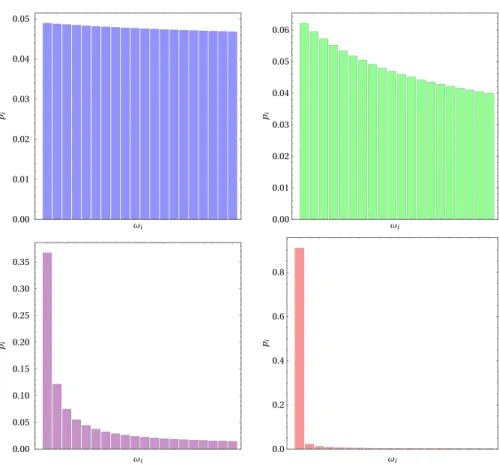
the reported results display the fraction of energy content in each mode for a system with N ¼ 20, that is, 21 normal modes and different values of the energy injection rate. It is quite clear that the larger the energy injection rate S, the stronger the deviation from energy equipartition, with increasing energy concentration in the lowest-frequency mode ω0. This energy concentration phenomenon, which we can call phonon condensation, stems from the classical Liouville equation and displays several analogies with the phenomenology of the pseudo-Bose condensation predicted by Fröhlich in a quantum framework and
FIG. 1. Classical Fröhlich-like condensation. Normalized fractions of energy pi in normal modes vs the mode frequencies of the
system Isysfor a fixed number of modes: N ¼ 20. The histograms display increasing deviations from energy equipartition among the
normal modes as the energy input rate S increases. The spectra correspond to S ¼ 0.1 (blue), S ¼ 1 (green), S ¼ 10 (purple), and S ¼ 100 (pink). Equipartition corresponds to equal heights of the bars. Note the great difference among the energy fractions in the lowest normal mode and in the higher frequency modes.
subsequently largely studied and debated in the same quantum framework.
A relevant feature of the Fröhlich condensation is the existence of a threshold in the energy injection rate, which corresponds to the breaking of the above-discussed per-mutation symmetry. In order to find out if a similar threshold effect is also displayed by our classical model, we study the behavior of the above-defined indicators of symmetry breaking (the condensation index Ey and the ratio yωi=yω0) as a function of S and for different values of
N. Figure 1 shows that, for the chosen values of S, it is pi> piþi; hence, the parameter p1=p0appears as a natural choice to detect a possible threshold effect. The results of numerical simulations of the order parameters have been reported in Fig.2. Both indicators pass from their respec-tive equipartition values (Ey≃0, p1=p0≃1) to their con-densation values (Ey≃1, p1=p0≃0) by displaying a clear steepening at increasing N. In particular, at increasing N, the curves of the condensation index EyðS; NÞ display a tendency to superpose at large S values, and a sharpening of the transition knee at lower S values, suggesting an
asymptotic convergence to a sharp bifurcation pattern. In fact, this sharpening of the transition curves with N is reminiscent of the finite-size patterns of the order parameter as a function of the control parameter of equilibrium second-order phase transitions. An analogous phenomenon is displayed by the S pattern ðp1=p0ÞðSÞ of the indicator p1=p0 at increasing N. Actually, the right panel of Fig.2
shows that, around the value S≃10, the different curves ðp1=p0ÞðS; NÞ cross each other and get steeper at increas-ing N, again suggestincreas-ing that the larger the number of modes the sharper the transition between almost equipartition among the modes and phonon condensation in the low-est-frequency mode. It is worth noting that this phenom-enology is qualitatively confirmed by the outcomes reported in Fig. 5 (aimed at highlighting a saturation effect), where again a sharpening—at increasing N—of a threshold effect can be observed. The lower panel of Fig.2, for the case of Nsys¼ 201, provides some interesting and more detailed information about the dynamics underlying the condensation phenomenon reported in the upper panels of the same figure. In fact, the lower panel shows how the
FIG. 2. Classical Fröhlich-like condensation. For an increasing number of modes entering the numerical simulations of Eq.(4 9), in the upper left panel, the condensation index Ey, defined in Eq.(50), is reported versus the energy input rate S, and in the upper right panel,
the ratio of the energy content p1=p0is reported versus S. At equipartition, E0¼ 0 and p1=p0¼ 1; for the condensed state, Ey¼ 1 and
p1=p0¼ 0. The colors of the lines correspond to Nsys¼ 11 (blue), Nsys¼ 21 (green), Nsys¼ 41 (brown), Nsys¼ 101 (orange),
Nsys¼ 201 (purple), and Nsys¼ 301 (red). The dashed oblique line (tangent to the inflection point of the two highest N curves) is a
guide to the eye to mark a possible asymptotic bifurcation point. In the lower panel, the relative energy content of two groups of modes —pi for i ¼ 0–10 (from blue to purple) and i ¼ 99, 100, 101 (blue, green, magenta superposed)—are displayed as a function of S,
relative energy content piof a randomly chosen subset of modes (p0, p1, p5, p10, p100) deviates from energy equipartition at increasing S. We can observe that the highest frequency mode selected, p100, deviates from equipartition at smaller values of S than the lower fre-quency modes chosen; then, somewhat below S ¼ 10, the energy content of all the selected modes starts decreasing, except the energy content p0of the lowest-frequency mode, which gathers more and more energy, approaching the value p0¼ 1, that is, full condensation at high S.
The main result of this theoretical part of the paper is an original derivation of a classical counterpart of the well-known Wu-Austin quantum Hamiltonian from which Fröhlich’s rate equations can be derived. This classical counterpart consists of a system of nonlinear dynamical equations (4 9) for the (adimensionalized) energy content yωi of each normal mode ωiof an ensemble of oscillators
coupled with two thermal baths at different temperatures. The ensemble of oscillators—ideally modeling the vibra-tions of the atoms or of groups of atoms in a macromolecule —is both linearly and nonlinearly coupled to the set of oscillators representing a thermal bath at temperature TB; this thermal bath accounts for the environment (mainly water molecules) and for other fast internal oscillations of a macromolecule. The second thermal bath at a temperature TS≫ TB models an external energy supply, in close analogy with the Wu-Austin model. The numerical study of Eq.(4 9)has shown that the condensation phenomenon is not peculiar of a quantum model, which a priori was not an obvious fact; hence, the occurrence of a phonon conden-sation phenomenon in a macromolecule at room temper-ature is more plausible in our classical model than in Fröhlich’s quantum model. Therefore, even though Eq.(4 9)
still represents a biomolecule in a very idealized way, the genericity of qualitative features of out-of-equilibrium phase transitions—mentioned at the beginning of this section— suggests that the condensation phenomenon should actually occur in real biomolecules, even though our model is not expected to predict the quantitative details of the phenome-non. This is enough to make the predicted phenomenology worth an effort for its experimental detection.
III. EXPERIMENTAL DETECTION OF NONEQUILIBRIUM COLLECTIVE MODE Even though experimental evidence of the existence of collective modes of vibration of biomolecules was provided at thermal equilibrium by means of Raman spectroscopy[1]
many years ago and is still the object of many investigations
[2–7,31], no experimental evidence is available for the possibility of exciting out-of-thermal-equilibrium collective oscillations of a biomolecule. Unveiling whether these can be activated amounts to understanding whether a necessary condition to activate long-range intermolecular electrody-namic forces[8]can be fulfilled. This strongly motivated the joint theoretical and experimental work reported in the
present paper. The experimental counterpart of the theoreti-cal work relies on two complementary experiments.
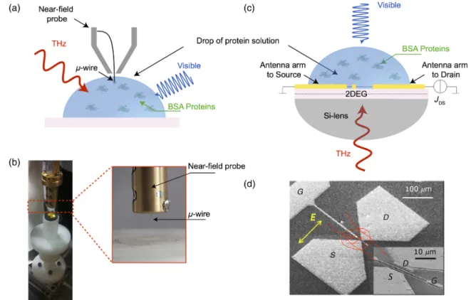
For both experiments, a model protein has been chosen: the BSA protein. This protein is mainly made out of α helices and is a “model” since it is largely studied in the biophysical chemistry literature. Our strategy to create a stationary out-of-thermal-equilibrium state of this molecule is to induce it by means of optical pumping—without involving any optical transition of the protein—through the excitation of some fluorochromes bound to each protein molecule. The optical excitation of these fluorochromes creates, on each protein, some “hot points” acting as the epicenters of a so-called “proteinquake” [32,33] —dis-cussed in more detail later—and resulting in an energy transfer to the vibrational part of the protein. We used the Alexa4 88 fluorochrome, which is covalently bonded at the lysine residues of the BSA and which is excited by means of an argon laser (wavelength 4 88 nm). Some 0.19 eV per fluorochrome and per incident photon (the average energy difference between the absorbed and reemitted photons) is thus available for an energy transfer to the protein and, partly, to its environment. By attaching an average number of 5 fluorochromes per protein, a considerable amount of energy (≫ kBT) can be continuously pumped into each protein. Two THz-near-field absorption spectroscopy set-ups of aqueous solutions of the protein (at 1 mg=mL concentration), operating in two distinct laboratories, have been used at room temperature [Figs.3(a)and3(c)]. In both experiments, THz radiation is produced by tunable, highly spectrally resolved (< 300 Hz) and continuous-wave sources, with an average power of 1 mW, allowing an accurate detection of possible resonances. A typical experi-ment consists in three phases; during each of them, the aqueous solution of proteins is illuminated with THz radiation, performing a sweep in frequency and thus allowing us to measure the frequency dependence of the absorbed electromagnetic power (detected by the near-field probes) in the solution. During the first phase, no extra illumination is done with the argon laser; during the second phase, the argon laser is switched on to excite the fluorochromes bound to the proteins; finally, during the third phase, the laser is switched off to check whether some memory and irreversible photochemistry effect (photo-bleaching) or sample heating is present. The use of near-field coupling of metal probes to the sample eliminates the Fabry-Perot interferences often seen in optical spectra in fluidic cells[34 ].
The first setup [Figs. 3(a) and 3(b)] includes a micro-coaxial near-field probe inside a metallic rectangular waveguide, enabling a modal transition from TM01 Sommerfeld’s to TE01 waveguide mode. The subwave-length diameter of the wire (12 μm) allows an extremely localized detection of the longitudinal component of the electric field at its end and in a volume of about 4 pL. The spectra were subtracted from the spectrum of pure water in
order to remove artifacts coming either from the water absorption or from the geometry of the experimental setup. The second setup[35][Figs.3(c)and3(d)] involves a near-field probe rectenna composed of a planar metal bow-tie antenna, with dimensions close to half a wavelength (at 0.3 THz), that enhanced the THz field in the feed-gap region (volume of about 0.2 pL) and a plasma-wave field-effect transistor (FET) integrated in the feed gap of the antenna. When illuminated by THz radiation, the antenna-coupled FET device provides a dc voltage—between source and drain contacts—proportional to the THz-field intensity[36–38]. A hemispherical silicon lens pressed on the back of the semiconductor substrate focuses the THz radiation on the antenna, simultaneously eliminating Fabry-Perot interference in the substrate[39]. The spectrum of the protein solution obtained in the absence of blue light illumination is subtracted from the spectrum obtained with blue light illumination.
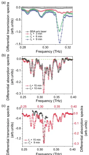
Figure 4 (a) presents the spectra obtained using the microcoaxial probe in the absence of blue light illumination (black squares) and in the presence of blue light illumina-tion of different duraillumina-tions (from 3 to 9 min). In the former case (no illumination), there was no specific spectral feature in the studied frequency range, while in the latter case (with illumination), we observed spectral resonances that become more evident for an increasing duration of illumination. In particular, the strongest resonance appeared at 0.314 THz,
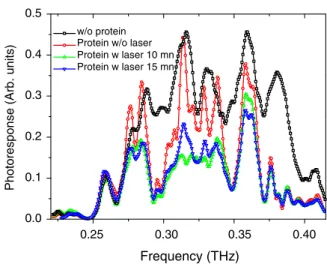
accompanied by two other minor resonances situated at 0.278 and 0.285 THz; these values did not depend on the time of illumination, and the strength of the resonances saturated after 9 min of illumination. These results have full reproducibility. Figure 4 (b) presents the spectra obtained using the rectenna probe for two durations of blue light illumination. The spectra with illumination on versus illumination off were taken several times (two of them showed reproducibility). In this case, we also observed the appearance of evident resonances whose strength saturated at increasing durations of illumination (10 and 15 min in the two experimental runs reported). Long excitation times are needed because, under our experimental conditions, the energy dissipation rate and the energy supply rate are almost equal, so a long time is needed to accumulate enough energy into each protein in order to make intra-molecular nonlinear interaction terms sufficiently strong to activate the condensation phenomenon.
The spectra obtained using the two previously described methods and for the longer durations of illumination are compared in Fig. 4 (c). The principal resonance at 0.314 THz is perfectly reproduced using two completely different and complementary setups. Since THz extinction in water is huge (2000 dB=cm), the emergence of this spectral feature of the protein out of the water absorption background must be associated with the activation of a giant dipole moment. This can happen only as a
FIG. 3. Experimental setup of THz absorption near-field spectroscopy. (a) A drop of the biological sample placed under the near-field probe, which is directly immersed in the solution. (b) Picture of the near-field probe and its microwire. (c) A drop of the biological sample placed above the near-field rectenna. (d) Electron-beam microscopy picture of the bow-tie antenna with its integrated FET.
consequence of the activation of a coherent oscillation of the whole molecule, possibly together with a dipole-moment strengthening due to an electretlike structuring of water dipoles of the first hydration layers of the proteins, as the hydration shell might contribute to the magnitude of the protein dipole moment[4 0].
Since the BSA is a heart-shaped globular protein, the possible lowest frequency of a global oscillatory mode is roughly estimated by schematizing the molecule as com-posed of two masses m, equal to half the total protein mass, joined by a spring of elastic constant k given by k ¼ EA0=l0, where E is the Young modulus of the protein,
and A0 and l0 are its transverse section and length at rest, respectively. Using m ¼ 33 kD, A0≃1.2 × 10⁻¹³ cm2, l0≃1.2 × 10⁻⁷ cm, and E ¼ 6.75 GPa, we find ν ¼ ð1=2πÞpffiffiffiffiffiffiffiffiffik=m≃0.300 THz, which is close to the main resonance observed at 0.314 THz. Since the BSA molecule can be modeled to first order as a three-dimensional elastic nanoparticle[6], a more refined approximation is obtained by modeling the protein with an elastic sphere and then considering its vibrational frequencies.
The fundamental frequency of a spheroidal deformation mode of an elastic sphere is given by the formula[4 1]
ν0¼ ð1=2πÞ½2ð2l þ 1Þðl − 1Þ&1=2 ' E ρR2 H (1=2 ; ð51Þ which holds for l≥2. For the lowest mode (l ¼ 2), we find the frequency ν0¼ 0.308 THz, which agrees within an error of about 2% with the observed peak value at ν ¼ 0.314 THz, using the following data for the BSA protein: Young modulus E ¼ 6.75 GPa obtained at room temperature using Brillouin light scattering of hydrated BSA proteins [4 2], hydrodynamic (Stokes) radius RH ¼ 35 Å, and specific volume 1=ρ ¼ 0.74 derived from small-angle x-ray scattering (SAXS) experiments [4 3]. Though such a modeling is unrealistic since it does not take into account the details of the protein structure and the associated normal modes [4 4 ], it nonetheless catches a relevant aspect of the global deformation dynamics of the BSA molecule, namely, the activation of a collective oscillation, also suggesting that the physical parameters adopted correspond quite well to the situation investigated
[4 5]. Secondary resonances are also present in both spectra. We could tentatively give a possible explanation by considering torsional modes. These could be activated at the frequencies given by the relation[4 1]
νt¼ ν0 ' ð2l þ 3Þ 2ð2l þ 1Þ (1=2 ; l≥2;
where ν0is given by Eq.(51), whence, for l ¼ 2 and l ¼ 3, one finds ν ¼ 0.257 THz and ν ¼ 0.246 THz, respectively. These could be associated with the two weaker absorption lines observed at ν ¼ 0.278 THz and ν ¼ 0.285 THz. Here, the larger discrepancy can be attributed to the nonspherical shape of the BSA, which entails the existence of different moments of inertia according to the rotation axis, whereas the breathing mode is insensitive to this. Minor peaks are observed at higher frequencies with the rectenna (falling outside the accessible frequency range of the near-field probe) when the protein solution is illumi-nated with blue laser light. However, the blue light illumination could produce spurious signals from the 2D electron gas of the FET junction as a consequence of electron-hole pair excitation causing a change of the transistor channel conductivity. This effect is well known (a)
(b)
(c)
FIG. 4 . Differential transmission and absorption spectra as functions of the frequency. (a) Spectra obtained using the microwire probe after subtraction of the water spectrum in the absence of illumination and in the presence of illumination for the reported durations. (b) Spectra obtained using the rectenna, after subtraction of the protein solution without illumi-nation, for the reported durations. (c) Comparison of the two normalized spectra for the longest illumination durations.
and studied in the literature[4 6], so minor peaks could be instrumental artifacts due to this electron-hole-pair creation effect.
Let us stress an important point: Computational normal mode analysis for proteins has shown nearly continuous vibrational density of states [4 4 ], which have also been proven to be nearly uniformly optically active. Moreover, the coupling of these vibrational modes with water results in broad absorption features [4 7,4 8]. But this is true at thermal equilibrium, whereas in out-of-equilibrium phonon condensation, the energy content of all the normal modes is strongly depleted, with the exception of the collective mode, hence a narrow absorption feature. In fact, the computation of the function LðωÞ in Sec. IV shows how a dipole actively oscillating at a given frequency entails an absorption feature of shape similar to the experimentally observed one.
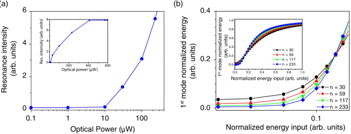
According to our classical version of the Fröhlich model, it is also expected that the appearance of a collective oscillation should exhibit a thresholdlike behavior when increasing the energy flowing through the protein. Actually, Fig.5(a) presents a clear threshold in the intensity of the resonance peak at 0.314 THz when the optical input power exceeds 10 μW. By using a classical formalism for the analysis of the out-of-equilibrium phonon condensation, we have calculated the intensity of the normal vibrational modes of the BSA protein as a function of the source power injected through the protein. Figure 5(b) highlights the thresholdlike behavior of the intensity of the fundamental mode that accumulates the energy at the expense of the excited modes, in qualitative agreement with the exper-imental outcome. By increasing the number of modes included in the calculation, this threshold becomes more and more evident. The experimental and theoretical results reported in Fig. 5 also show the same saturation effect occurring at large values of the energy input rate.
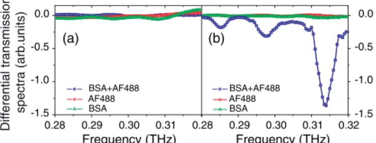
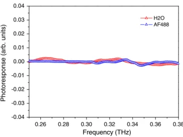
The observed spectra are certainly due to the light-excited protein because the spectral feature at 0.314 THz is not observed by illuminating (i) water alone, (ii) an aqueous solution of the fluorochrome in the absence of the protein, or (iii) an aqueous solution of the BSA protein without the bound fluorochrome (see Sec.IV). On the other hand, the observed spectral line at 0.314 THz immediately disappears by switching off the laser. Remarkably, the spectra obtained with two independent and different experimental setups, based on two different methods of detection of the THz radiation, operated in two different laboratories, show a strikingly good overlap of the respective absorption line profiles at 0.314 THz. This result is in excellent agreement with the frequency of 0.308 THz predicted for the sphe-roidal (collective) vibrational mode computed on the basis of recent experimental measurements of the relevant parameters of the BSA protein. This triple concordance among the results obtained so far should be enough to exclude experimental artifacts. Nevertheless, various sources of the artifact for the observed phenomenology were considered. One objection is that the observed phenomenology is just a trivial heating effect due to the laser light. This would be true in the absence of a frequency-dependent response to the injection of energy into the proteins. Heating indeed means increasing the kinetic energy of the atoms and groups of atoms of the protein, entailing energy equipartition among the vibra-tional modes of the protein. Hence, neither a frequency-dependent effect nor a threshold effect for the energy input rate would be measured, but a new thermal equilibrium state would be achieved. To the contrary, each protein— submitted to continuous energy feeding and energy dis-sipation—behaves as an open system undergoing a non-equilibrium phase transition: When the ratio between energy gain and loss exceeds a critical value, a collective behavior sets in, producing the phonon condensation, as
n = 30 n = 59 n = 117 n = 233
1
st mode normalized energy
(arb. units)
0.0 0.2 0.4
Normalized energy input (arb. units) 0.1 0.0 0.2 0.4 0.6 0.8 1.0 0.0 0.2 0.4 0.6 0.8 1.0 n = 30 n = 59 n = 117 n = 233 Nor m ali ze d en erg y of 1 st m od e (arb . un its)
Normalized source power (arb. units)
Optical Power (µW)
Resonance
intensity
(arb. units) 1 Normalized energy input (arb. units)
st mode normalized energy
(arb. units) (a) (b) 0.1 1 10 100 0 2 4 6
FIG. 5. Thresholdlike behavior of giant dipolar oscillations. (a) Intensity of the resonant peak measured at 0.314 THz as a function of the optical laser power. (b) Normalized energy of the fundamental mode calculated as a function of the normalized source power. The different curves correspond to the reported numbers of normal modes of the BSA protein. Theory and experiment are in qualitative agreement.
has already been discussed in Sec.II. Then, an important point concerns the conversion mechanism of the visible light energy absorbed by the electrons of the complex protein or dyes into the vibrational modes of the proteins. This mechanism of rapid intramolecular dissipation of energy through quakelike structural motions as a conse-quence of a perturbation (such as the breaking of a chemical bond or the absorption of photons through electronic transitions) is receiving increasing experimental attention
[32,33,4 9,50] and is referred to as the “protein quake.” Similar to an earthquake, this effect describes how a protein strain is released at a focus or “hot point” (in our case, the fluorochromes) and then rapidly spreads as a structural deformation through waves, thus exciting protein vibra-tional modes. Another source of artifact could be the apparition of standing waves and related interferences, but these would be easily identified. Furthermore, there is no reason for such interferences—if they exist—to manifest themselves as a consequence of the excitation of fluoro-chromes through the blue light [see Fig. 6(b)].
IV. MATERIALS AND METHODS A. Sample preparation
BSA was purchased from Sigma-Aldrich (A7030) (St. Louis, MO) in lyophilized powder—protease free, fatty acid free (≤0.02%), essentiallyglobulin free; since the degree of purity of the BSAwas higher than 98%, it was used without further purification and was dissolved directly into bidistilled water.TheBSAmoleculeswerelabeledwiththefluorochrome AF4 88 5-TFP (Alexa Fluor 4 88 Carboxylic Acid, 2, 3, 5, 6— Tetrafluorophenyl Ester), 5-isomer (A30005), which was purchased from Molecular Probes Invitrogen.
The dye has excitation/emission of 495=515 nm and a molar extinction coefficient of ε495¼ 71 000 M cm−1. Both the protein and dye concentrations have been
determined by measuring their absorbance with a Nanodrop 1000 Spectrophotometer (ThermoScientific) at 280 nm with a molar extinction coefficient of 36 000 M cm−1 and at 4 95 nm with a molar extinction coefficient of 71 000 M cm−1, respectively. The chemically labeled BSA molecules were obtained by homemade labeling using a 2 mg=mL aqueous solution concentration of proteins with an initial ratio of concentrations [A4 88 5-TFP]/[BSA] equal to 8 in sodium bicarbonate at a pH≈8.5, during one hour. Unconjugated dye was removed using a PD-mini-trap G25 (GE Health Care) according to the instructions of the manufacturer, using gravity protocol, and the degree of labeling was determined spectroscopically. After purification, each BSA molecule has between 5 and 6 fluorochromes attached.
B. Experimental detection of the collective mode Two separated and different experiments, performed in Montpellier (France) and in Rome (Italy), respectively, have been performed to obtain the terahertz nonequilibrium spectra of the model protein chosen. The former used a microwire as a local probe, whereas the latter used a nanorectenna.
1. Microwire-based THz spectroscopy
A constitutive element of the experimental setup is a tunable and continuous-wave primary source from Virginia Diodes Inc. [51], thus emitting in the 0.22–0.33-THz frequency range with an average power of 1 mW. The high spectral resolution (< 300 Hz) of the continuous-wave source allows an accurate detection of resonances. The emitted radiation beam is focused on the samples of protein solutions on which a 4 88-nm light beam—pro-duced by an argon laser—can be focused too and switched on and off at willing. The blue light provides the proteins with the necessary energy to activate a collective vibra-tional state. The latter is an out-of-equilibrium state because it is kept by a nonthermal energy supply.
The THz near-field scanning spectroscopy technique in aqueous medium is performed by resorting to a homemade microcoaxial (i.e., subwavelength) near-field probe put inside a metallic rectangular waveguide connected to a heterodyne head and an electrical spectrum analyzer. The subwavelength diameter of the wire allows an extremely focused enhancement of the longitudinal component of the electric field at its end over a volume of 4 pL. In 1995, Keilmann[52]highlighted the advantages of introducing a metal wire in a circular metal waveguide to produce probes for near-field microscopy in the far-infrared and microwave frequency domains. The advantage of this method is to avoid the frequency cutoff when the diameter of the guide is a subwavelength one. The circular waveguide is trans-formed into a coaxial waveguide, which does not have a low-frequency cutoff and which makes superfocalization and high-resolution imaging possible.
0.28 0.29 0.30 0.31 Frequency (THz) Frequency (THz) 0.28 0.29 0.30 0.31 0.32 -1.5 -1.0 -0.5 0.0 -1.5 -1.0 -0.5 0.0 (a) (b) BSA+AF488 AF488 BSA BSA+AF488 AF488 BSA noi ssi ms na rt l ait ne ref fi D )st in u. br a( art ce ps
FIG. 6. Differential transmission spectra of the microwire-based absorption spectra. (a) Without blue light illumination (laser OFF), obtained with solvated AF4 88 in water (red circles), solvated nonlabeled BSA in water (green triangles), and BSA labeled with AF4 88 solvated in water (blue squares). (b) With blue light illumination (laser ON), obtained with solvated AF4 88 in water, at a concentration of 5 mg=mL (red circles); solvated nonlabeled BSA in water (green triangles); and BSA labeled with AF4 88 solvated in water (blue squares). Labeled and nonlabeled BSA concentrations are kept equal to 1 mg=mL.
However, for the experiments reported in the present work, a rectangular waveguide is used, and this entails some different phenomena since the microwire is soldered along the long axis of the waveguide and bent to exit it. This has two main consequences: On the one hand, the microwire enables a modal transition, and on the other hand, it serves as a waveguide. The bent portion of the microwire allows the conversion of the fundamental mode TE01 inside the rectangular waveguide into a TM01 mode along the wire. To optimize the coupling efficiency between the near field and the probe, special care is taken for the positioning of the microwire inside the guide. More precisely, the maximum of the near-field signal is theo-retically attained for a wire positioned at Linside¼ p½ðλTE01Þ=4& from the open side of the waveguide, where
λTE01 is the wavelength of the TE01mode at the considered frequency. At 0.3 THz, the microwire must be fixed at an entire multiple p of 250 μm. The best compromise between efficiency and technical possibilities is found for p ¼ 4, which gives Linside ¼ 1 mm. The second parameter to take into account is the angular positioning of the bent portion of the microwire inside the rectangular waveguide. The coupling is at a maximum when the wire is parallel to the orientation of the electric field in the guide, that is, along the long axis of the rectangular waveguide. Finally, we note two relevant parameters, which are the total length and the diameter of the wire. The intensity of the electric field is roughly sinusoidal, and its maximum is attained when the total length L is a multiple of the half-wavelength. The best compromise between theory and technological possibilities has given a total length of L ¼ 2 mm. Since the electric-field intensity at the microwire extremity increases when the diameter decreases, we use a wire of 12 μm diameter. All the previously mentioned parameters have also been simulated using CSTmicrowaves studio® (https://www.cst.com/products/cstmws) to ensure the best coupling efficiency possible.
All the measurements have been performed at room temperature. A drop of the protein solution sample is placed under the near-field probe, which is directly immersed inside the solution. A typical experiment consists in measuring the near-field electric-field intensity through a reference medium (water) and the protein solution sample. A sweep through the frequency domain accessible to the THz source is performed both when the blue light is switched on and off to yield a difference spectrum showing the absorption features that are attributed to collective vibrations of each protein molecule.
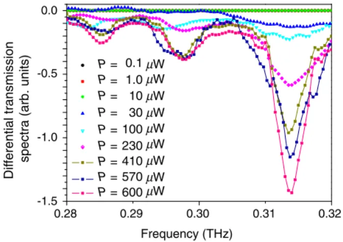
Figure7displays the spectra, stabilized in time, obtained by varying the power of the laser illuminating the solution of labeled proteins at a constant concentration of 1 mg=mL. Notice that the secondary peaks appear and develop together with the main peak at 0.314 THz; therefore, these secondary peaks are also vibrational modes of the entire protein, giving some support to the hypothesis attributing
them to torsion modes. However, these kinds of modes cannot be accounted for by our theoretical model because it contains no explicit information about the geometry of the molecule.
2. Rectenna-based THz spectroscopy
In order to minimize the optical depth of water, in the second experiment (Rome), the probe domain was reduced to a volume of 10 × 10 microns in xy(horizontal plane) and to about 2 microns in z (vertical axis). To confine the THz radiation (wavelength λ around 1 mm) to such a deeply subwavelength region, a plasmonic antenna is used[35]. This device is based on two main components: a planar metal antenna with length close to λ=2 (bow-tie, broadband type) that produces a high THz field region with an antenna feed gap of 10 × 10 microns; and a plasma-wave FET transistor, which is a THz nonlinear electronic device integrated in the feed gap of the antenna that provides an electric signal proportional to the THz field strength in the feed gap only. The plasma-wave transistor was first introduced by Dyakonov and Shur in 1993[36]and further developed by many authors[37], the main advantage being that standard microwave transistor technology can be employed for fabricating a device that is sensitive to THz radiation. The device is mounted in a package with a silicon lens pressed on the back of the semiconductor substrate and illuminated from below with a tunable THz oscillator (by Virginia Diodes Inc., 0.18–0.4 THz) through a set of off-axis parabolic mirrors. The resolution of the free-running oscillator is 2 GHz. After acquiring the empty-channel response spectrum of the device, a drop of protein solution was cast on the top (air) side of the device with a micropipette (a volume of 1 microliter was drop-casted). The drop extends over the entire antenna; however, the radiation comes from below (i.e., from inside the substrate), and it is not attenuated by the whole drop. In this
P = µW µW µW µW µW µW µW µW µW P = P = P = P = P = P = P = P = Dif
ferential transmission spectra (arb. units)
Frequency (THz) 0.28 0.29 0.30 0.31 0.32 -1.5 -1.0 -0.5 0.0 0.1 1.0 600 570 410 230 100 30 10
FIG. 7. Differential transmission spectra of the microwire-based absorption spectra obtained with different excitation power of the laser. The labeled BSA concentration is kept fixed at 1 mg=mL. The first three spectra are exactly superposed.