Composition of fine and ultra-fine particles and source identification by stable isotope ratios

COMPOSITION OF FINE AND ULTRA-FINE PARTICLES AND

SOURCE IDENTIFICATION BY STABLE ISOTOPE RATIOS

Jec-Kong Gone

M.S., Department of Nuclear Science National Tsing-Hua University, Taiwan, 1989

SUBMITTED TO THE DEPARTMENT OF NUCLEAR ENGINEERING IN PARTIAL FULFILLMENT OF THE REQUIREMENTS FOR THE DEGREE OF DOCTOR OF

PHILOSOPHY INMJMHY IN rSMAY _NUCLEAR

ENGINEERING AT THE

MASSACHUSETTS INSTITUTE OF TECHNOLOGY JUNE 1998

© Massachusetts Institute of Technology, 1998. All rights reserved.

Signature of Author: ... .... ... Departent of Nuclear Engineering, May 15, 1998

Certified by ...

V / Ilhan Olmez

Principal Research Scientist, Nuclear Reactor Laboratory, Thesis Supervisor

Accepted by : ...

Glen R. Cass Professor of Environmejtal Engineering Science, California Istitute of Technology

Thesis Reader Accepted by :... ... ...

7 Kevin W. Wenzel

Assistant Professor of Nuclear Engineering, Thesis Reader

Accepted by ...

Lawrence M. Lidsky Chairman, Departmental Committee on Graduate Students

ixe_

COMPOSITION OF FINE AND ULTRA-FINE PARTICLES AND

SOURCE IDENTIFICATION BY STABLE ISOTOPE RATIOS

by

Jec-Kong Gone

Submitted to the Department of Nuclear Engineering on May 15, 1998 in Partial Fulfillment of the Requirements for the Degree of Doctor of Philosophy

in Nuclear Engineering ABSTRACT

Fine (da < 2.1 Rm) and ultra-fine (da < 0.1m) atmosphere particulate samples collected from two

sites in the United States were analyzed for elemental compositions by Instrumental Neutron Activation Analysis (INAA) at Massachusetts Institute of Technology. The eastern site samples were collected at the Great Smoky Mountain National Park from July 15 to August 25, 1995. The western site samples were collected from a rooftop in Pasadena, California over one winter month in January/February, 1996. Elemental concentrations determined by INAA for the eastern site samples were compared with results from samples (da <2.4 [im) collected concurrently but analyzed by other techniques. The results showed consistency between different analytical techniques. Factor Analysis

(FA) and Absolute Factor Score-Multiple Linear Regression (AFS-MLR) methods were used to

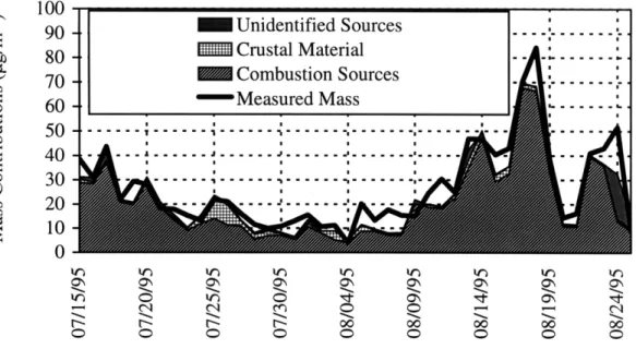
identify sources and their contributions to fine particulate samples at the eastern site. The results showed that the crustal contribution to fine aerosol mass was significant around July 24-26, 1995, and the coal combustion contribution peaked around August 14-18, 1995. The average contribution from crustal sources to the fine particulate mass was 7+3 % for the 2.1 pm samples and 11+4 % for

the 2.4 pm samples. The mass difference may be due to the different maximum size of the particles.

The average contribution from combustion sources was 77+4 % for the 2. 1m samples and 90+6 % for the 2.4 gm samples. Elemental patterns were used to identify sources of ultra-fine particles. Motor vehicle emissions might be the cause of the increase in the ultra-fine particle concentration of Al and Fe at the western site.

Variations in stable isotope ratios of 130Ba/138Ba, 121Sb/123Sb, 84_Sr/86_{Sr and} 79_Br/81_{Br were investigated} using INAA. This technique was applied to fine particulate samples with sources identified by FA. The results showed that the 130_Ba/138_{Ba ratio of the dust sample was 0.00151+0.00008, and the ratio}

was 0.00109+0.00003 for the combustion sample. This suggests that the 130Ba/138Ba ratio can be used to separate contributions from soil and combustion sources even if they have similar chemical compositions. Crustal material may have a lower 121_Sb/123_{Sb ratio than the combustion source of fine} particles. The 84

Sr/86Sr and 79Br/81Br ratios also showed differences between these samples, but the differences were not greater than the statistical uncertainty of the measurements.

Thesis Supervisor: Dr. Ilhan Olmez

Acknowledgements

This work could not be done without great help from Dr. Ilhan Olmez. His constant support and friendly advice have made the research possible. His wisdom provided me the right direction for the accomplishment, and it was my great honor to work with him for the past five years. I also thank Dr. John Bernard and the MIT research reactor team for their help. Dr. Bernard not only helped me with my research, but his humor also smoothed all the odds that I faced in the past few years. I owe great thanks to the people from the Environmental Research and Radiochemistry group of the Nuclear Reactor Laboratory at Massachusetts Institute of Technology. Mrs. Jianmei Che and Dr. Michael Ames helped me to settle the experiment and running sample analysis. Their constant support made this research an excellent experience. Mr. Francis Pink, Dr. Jack Beal, and Dr. Gulen Gullu helped me with data interpretation. Their knowledge and experience gave me great inspiration for my work. I also thank Miss. Lara Hughes and Professor Glen Cass from the California Institute of Technology to provide me size-segregated CIT/MOUDI samples, and great thanks to Professor Lynn Hildemann from the Stanford University who provided me the 2.1gm MIT/SU samples. Professor Peter McMurry and his group from the University of Minnesota helped me with sample collection at the Great Smoky Mountain National Park, and I also thank him to have provided me the UMn/MOUDI samples. I appreciated Dr. Stefan Musarra, Dr. Pradeep Saxena from the Electric Power Research Institute, and Dr. Thomas Cahill from the University of California at Davis to provide me the NPS/IMPROVE data. I thank Professor Sidney Yip from the Department of Nuclear Engineering for his friendly help. His advice has made my graduate study easier at the Massachusetts Institute of Technology.

Support from friends has made my study a wonderful experience. I thank Mr. Kuo-Shen Chen, Mr. Yu-Hsuan Su, Mr. Tsu-Mu Kao, Mr. Wen-Yih Tseng, Dr. Sinan Keskin and Dr. Xudong Huang for their friendships. Mr. Juane-Long Lin and Dr. Sol-II Su helped me with my settling. Their generosity was the best support on my first arrival.

Family is always my greatest assets. My beloved mother and uncle passed away during my graduate study, but support from my family helped me face all the odds. My father

was always there when I needed him. His spirit inspired me and his love gave me the courage to face all the challenges. My sister Jane and my brother Jimmy always gave me the best advice and helped me on everything. I could not have gone this far without their support. My fiancde Yuh-Mei Chen supported me all the time. Her love keeps my greatest comfort and her

TABLE OF CONTENTS Page ABSTRACT 2 ACKNOWLEDGEMENTS 4 TABLE OF CONTENTS 6 LISTS OF FIGURES 8 LISTS OF TABLES 11 Chapter 1 INTRODUCTION 13

Chapter 2 COMPOSITION OF FINE AND ULTRA-FINE PARTICLES 20

2.1 Sample Collection 20

2.2 Trace Element Analysis 25

2.3 Detection Limits of INAA for Different Elements 29

2.4 Experimental Results 31

2.5 Data Comparison 40

Chapter 3 SOURCE APPORTIONMENT OF FINE AND ULTRA-FINE

PARTICLES 46

3.1 Factor Analysis and Multiple Linear Regression 48

3.2 Source Apportionment of Fine Aerosol 52

3.2.1 Source Identification 54

3.2.2 Mass Regression and Crustal Contribution 58

3.2.3 Mass Contribution from Combustion Source and Origin of Sulfate 65

3.2.5 Elemental Source Contributions 72

3.3 Source Apportionment of Size-Segregated Impactor Samples 74 3.3.1 Source Identification of Impactor Samples 74

3.3.2 Depletion of Chlorine on Fine Aerosols 88

Chapter 4 SOURCE IDENTIFICATION BY STABLE ISOTOPE RATIOS 92

4.1 Element Selection 93

4.2 Stable Isotope Ratios for Selected Standards 94

4.3 Source Identification of Fine Particles by Stable Isotope Ratios 102

Chapter 5 SUMMARY 109

5.1 Thesis Summary 109

5.2 Recommendations for Future Work 115

REFERENCES 117

APPENDIX A ELEMENTAL CONCENTRATION DATA 125

APPENDIX B CALCULATED MASS CONTRIBUTION DATA 176

APPENDIX C THE INAA RESULTS OF SRM STANDARDS AND

LIST OF FIGURES

Page

Figure 2.1. Structure of Stanford University AIHL-Designed Sampler. 23

Figure 2.2. Structure of NPS/IMPROVE Sampler. 24

Figure 2.3. Structure of CIT/MOUDI Impactor Sampler. 24

Figure 2.4. MIT/SU 2.1 pLm samples time series plots of crustal elements. 34

Figure 2.5. MIT/SU 2.1 pLm samples time series plots of selected elements. 35

Figure 2.6. Comparison of elemental concentrations for MIT/SU with MOUDI and NPS

(if available) samples. 42-43

Figure 2.7. Comparison of elemental concentrations for MIT/SU with MOUDI and NPS

(if available) samples. 44

Figure 2.8. Time series plots of selected crustal elements (from MIT/SU & NPS). 45

Figure 2.9. Time series plots of selected anthropogenic elements (from MIT/SU &

NPS). 45

Figure 3.1. Source apportionment of fine aerosol by factor analysis and multiple linear

regression. 47

Figure 3.2. Histogram for calculation of most frequently occurring measured value. 53

Figure 3.3. Time series plot of Absolute Factor Scores of crustal factor using the

MIT/SU and NPS/IMPROVE data sets. 57

Figure 3.4. Time series plot of Absolute Factor Scores of combustion factor using the

MIT/SU and NPS/IMPROVE data sets. 57

Figure 3.5. Time series plot of Absolute Factor Scores of unidentified factor using the

MIT/SU and NPS/IMPROVE data sets. 58

Figure 3.6. Source contributions to fine aerosol mass as calculated by receptor modeling

using the MIT/SU data set. 59

Figure 3.7. Source contributions to fine aerosol mass as calculated by receptor modeling

using the NPS/IMPROVE data set. 59

Figure 3.8. Crustal material contributions to fine aerosol mass as calculated by receptor

summation of the masses of the oxides of the major measured crustal elements.

Figure 3.9. The percentage of the fine aerosol mass composed of crustal material as calculated by receptor modeling using the MIT/SU and NPS/IMPROVE data sets, and by the summation of the masses of the oxides of the major measured crustal elements.

Figure 3.10. Synoptic plot of general wind pattern between 07/24 and 07/26/95.

Figure 3.11. Synoptic plot of general wind pattern between 08/14 and 08/18/95.

Figure 3.12. The concentration of fine aerosol mass composed of combustion material as

calculated by receptor modeling using the MIT/SU and NPS/IMPROVE data.

Figure 3.13. The percentage contributions of sulfate to the combustion material as

calculated by receptor modeling using the MIT/SU and NPS/IMPROVE data.

Figure 3.14. Correlation of MIT/SU selenium with HEADS sulfate concentrations. Figure 3.15. Time series plot of sulfate to selenium ratio in fine aerosols.

Figure 3.16. Median, minimum, and maximum enrichment factors for elements measured in the MIT/SU samples by INAA.

Figure 3.17. The average concentrations of crustal elements in UMn/MOUDI and CIT/MOUDI Samples.

Figure 3.18. The average concentrations of rare earth elements in UMn/MOUDI and

CIT/MOUDI samples.

Figure 3.19. The average concentrations of elements with greater contribution from

anthropogenic emissions in UMn/MOUDI and CIT/MOUDI samples. 79-Figure 3.20. Concentration of crustal elements in UMn/MOUDI samples during dust

(07/25-07/29/95) and pollution (08/14-08/18/95) episodes.

Figure 3.21. Concentration of rare earth elements in UMn/MOUDI samples during dust

(07/25-07/29/95) and pollution (08/14-08/18/95) episodes.

-80

81

Figure 3.22. Figure 3.23. Figure 3.24. Figure 3.25. Figure 4.1. Figure 4.2. Figure 4.3. Figure 4.4.

Concentration of elements with greater contribution from anthropogenic emissions in UMn/MOUDI samples during dust (07/25-07/29/95)

and pollution (08/14-08/18/95) episodes.

83-Concentration distributions of Al, Fe, Sm and Sc on CIT/MOUDI samples collected for the last two runs.

Concentration distributions of La, Ce, and V on CIT/MOUDI samples collected for the last two runs.

The average concentration of Na and Cl on UMn/MOUDI and CIT/MOUDI Samples.

Schematics for sample counting on HPGe detectors.

Absolute efficiencies of the HPGe detectors at different energies.

Thermal neutron irradiation and counting diagram for integrated fine aerosol

samples in stable isotope study. 1

Absolute detector efficiency of HPGe detector used in determining fine

aerosol isotope ratios. 1

84 86 87 90 96 97 06 .07

LIST OF TABLES

Page

Table 2.1. Properties of aerosol samplers. 23

Table 2.2. The half-life, gamma energy and counting group of elements determined by

INAA. 28

Table 2.3. Minimum Detection Limit (MLD), average elemental concentrations and

standard deviations of MIT/SU 2.1 jtm samples. 30

Table 2.4. Summary statistics of MIT/SU 2.1 gim samples (ng/m3). 33

Table 2.5. Average elemental concentrations (ng/m3) and standard deviations among

the sample sets for each UMn/MOUDI size fraction. 36

Table 2.6. Average elemental concentrations (ng/m3) and standard deviations among

the sample sets for each CIT/MOUDI size fraction. 37

Table 2.7. Summary statistics of NPS/IMPROVE 2.4 jim samples (ng/m3). 38 Table 2.8. Average vapor and particulate phase atmospheric mercury concentrations. 39

Table 3.1. Sources of atmospheric particulates and their elemental markers. 50 Table 3.2. Most frequently observed values for elements in the MIT/SU and NPS

IMPROVE data sets (ng/m3). 53

Table 3.3. Varimax rotated factor loading matrix for the MIT/SU data set. 56

Table 3.4. Varimax rotated factor loading matrix of NPS/IMPROVE data set. 56

Table 3.5. Absolute (jig/m3) and percent mean aerosol mass contributions from identified sources as calculated by receptor modeling using MIT/SU and NPS/IMPROVE data sets, and by the summation of the masses of the oxides

of the measured major crustal elements. 63

Table 3.6. Mean calculated elemental source contributions (in ng/m3) to the measured fine aerosol concentrations based on the MIT/SU data. 73

Table 3.7. Mean calculated elemental or inorganic species source contributions

(in ng/m3) to the measured fine aerosol concentrations based on the NPS

Table 3.8. Cl/Na mass ratio of UMn/MOUDI and CIT/MOUDI samples at different stages.

91

Table 4.1. Potential elements and isotopes used for stable isotope ratio study. Table 4.2. Elemental concentrations of selected elements in standards. Table 4.3. Thermal neutron flux calculated using gold flux monitors. Table 4.4. Specific isotopic activities (counts/s g) determined by INAA Table 4.5. Isotopic ratios determined by INAA.

Table 4.6. Specific activity, isotopic ratio, and delta value of 130Ba/138Ba in each of the fly ash and AGV-1 Andesite samples.

Table 4.7. Experimental result of 130Ba/ 138Ba ratio on fly ash and AGV-1 samples

counted on the same HPGe detector.

Table 4.8. Element concentrations in 37mm Teflon® filter (ng/filter).

Table 4.9. Average enrichment factors of Br, Sr, Sb and Ba during crustal dust and

combustion episodes.

Table 4.10. Stable isotope ratios from integrated crustal and combustion samples.

94 95 97 100 100 101 102 103 104 107

Chapter 1

INTRODUCTION

Aerosols, the suspension of solid or liquid particles in a gas, such as air, are ubiquitous in our environment. Wind-blown dust, volcanic eruptions, vegetation and, of course, human activities all contribute to the generation of aerosols and each of these sources creates aerosols of different sizes and chemical compositions. Aerosols are known to play important roles in human health, light scattering and visibility change, cloud formation and in the energy balance of the atmosphere. Human activities have increased aerosol emissions which may increase toxic metal concentrations in the atmosphere (Galloway, et al., 1982). A recent study also shows that aerosols may be important for ozone depletion in the stratosphere because aerosols can provide significant surface areas for heterogeneous chemical reactions important for halogen chemistry (Solomon, et al., 1996). The U.S. Environmental Protection Agency (EPA) recently proposed new regulations (40 CFR Part 64) covering pollutant-specific emissions monitoring of aerosols (Ellis, 1997). A thorough

knowledge of the properties of aerosols is the first step to set regulations on their emissions and to protect our environment.

Aerosol sizes are usually classified in terms of their aerodynamic diameter (da). Aerodynamic diameter is the diameter of a unit density sphere (i.e. a water droplet, density

1g/cm3) having the same aerodynamic property as the particle in question. It is convenient to

think of aerosols as spherical particles which simplifies the calculations. However, except for the liquid droplets, aerosols may have many shapes. Size classification is usually done based on the particle settling velocity in the atmosphere. Particles with the same settling velocities are considered to be of the same size, regardless of their real sizes, compositions, and morphologies.

Particle size modes can be used to identify the particle's origins and the particle's chemical compositions may be important for health assessments. Whitby (1978) found that the size distribution of particles in urban atmospheric aerosols showed a trimodal distribution

with peaks around 0.015-0.04 gtm, 0.15-0.5 jim, and 5-30 gtm. Dodd et al. (1991) found additional size distributions depending upon the particles' sources, age, and atmospheric transformations by studying particles with da less than 2.5 jim from a rural site close to the Deep Creek Lake, Maryland. Particles with da less than 0.1 gim are called Aitken nuclei and are produced mostly from high temperature combustion processes or gas condensation (Fergusson, 1992). In this thesis, they will be referred to as ultra-fine particles.

Fine particles (da < 2.5 gm) originate mostly from the accumulation of smaller particles; coarse particles (da > 2.5 jm) are the products of a mechanical process such as erosion (Fergusson, 1992). The sizes of particles usually determine their lifetime in the atmosphere. Fine and ultra-fine particles are transported high into the troposphere and incorporated into raindrops. Wet deposition is therefore important for their removal from the atmosphere. Coarse particles, on the other hand, usually can not reach high altitude and are mainly removed by dry deposition. Gravitational settling can remove coarse particles and these particles' environmental impact is therefore more localized. In contrast, fine and ultra-fine particles may travel hundreds of miles before they are removed from the atmosphere by rain or impaction and their influence can be regional, even global.

Light scattering by particles is strongly dependent on their size and chemical composition. Visibility refers to the degree to which the atmosphere is transparent to visible light. Meteorologists use light extinction coefficients to quantify the visibility change. The light extinction coefficient is defined as the fraction of light that is reduced by scattering and absorption as it travels through a unit length of the atmosphere. It is dependent on the particle size distribution in the atmosphere (Reist, 1984). Fine particles scatter more visible light than coarse particles and have larger light extinction coefficients. The chemical composition of aerosols also affects light extinction (Ouimette et al., 1981). The extinction efficiency of elemental carbon in low humidity conditions is about three times larger than that of sulfates, nitrates, and organic carbon (Mathai, 1995) and it is about 17 times higher than that of coarse particles. Knowledge of the compositions of aerosols, especially fine and ultra-fine aerosols, is important in understanding visibility degradation.

Aerosol sizes have different human health impacts because of the geometry of the lung and the depth of penetration of these particles. Particles with an da less than 10 jim are

classified as inhalable particles. Coarse particles (da > 2.5 jim) are deposited in the nasopharyngeal region, and smaller particles (da < 2.5 jim) will deposit in the tracheobronchial region (Fergusson, 1990). Particles in the range of 0.1-1 jm can penetrate as far as the alveolar region. The heavy metal uptake by human blood can be very efficient for small particles. Fine particles (da < 2.5 jm) and sulfate may cause increased mortality in urban areas (Dockery, et al., 1993). Oberdorster et al. (1994) used TiO2 particles of 20 nm

and 250 nm diameters to study the correlation between particle size and lung injury. The result showed that the smaller particles caused a persistently high inflammatory reaction in the lungs of rats compared to the larger-size particles. This suggests that particle surface area may be more important than the total mass in regard to lung injury. Hall et al. (1992) estimated an increased risk of death of 1/10,000 in a year for the residents of the South Coast Air Basin of California and a loss of 1600 lives per year due to elevated inhalable particle mass. Oberdorster (1996) found that crystalline SiO2 shows a different dose response for lung

injury compared to other fine particles. This suggests that chemical composition also may be important for these particles. Sweet et al. (1993) found that toxic elements in da < 10 jim samples showed variations independent of particle mass. Chiou and Manuel (1986) found that most of Se, Te and other heavy volatile metals are in the fine aerosols, highlighting the importance of particle compositions. For especially fine and ultra-fine particles, it may be more important to base regulations on the particle's composition than total mass.

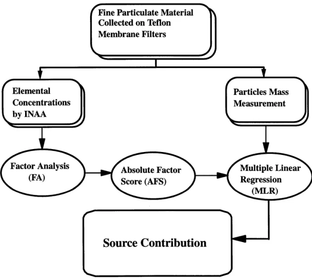
Because fine and ultra-fine particles are so important for environmental and human health issues, the first goal of this study is to determine their compositions. Instrumental Neutron Activation Analysis (INAA) is a very sensitive analytical technique that can determine more than 40 elements in a sample (Olmez, 1989; Parry, 1991). Samples are first irradiated with thermal neutrons, and then gamma rays emitted from activated nuclei are detected by High Purity Germanium (HPGe) detectors which have high energy resolutions. Because gamma rays are generated from each activated nucleus, the technique is sensitive to small amounts and can be used to measure elemental compositions down to absolute levels of a few nanograms. This analytical technique is used to determine the elemental concentrations of fine and ultra-fine particles in this study.

Compositions of fine and ultra-fine particles are also important because they can be used to identify their atmospheric sources. Atmospheric emissions from different sources have different elemental "signatures" especially with respect to their trace metal compositions (Olmez et al., 1996). Different models have been developed during the past few decades to assess source impacts in various regions. Traditional models such as dispersion models use input from emission sources and mass balance calculations to estimate impacts from suspended particulate matter and from other air pollutants. However, the physical and chemical processes in the atmosphere may change properties of aerosols. Even if dispersion models were correct, the source emission inventories upon which they rely are frequently not well known, or may change over time because of improved regulations. Receptor models, including chemical mass balances and factor analysis, have been used widely to assess impacts at a receptor site (Olmez et al., 1988, Olmez et al., 1996, Thurston and Spengler, 1985, Okamoto et al., 1990). Chemical Mass Balance models (CMB) assume that the emissions from various sources have different composition patterns and they can be separated by measuring the concentrations of many species in samples collected at a receptor site. However, CMB relies on the fact that all particles are primary and of the same composition as those released from the sources (Gordon, 1988). The CMB models are good for inactive species such as crustal elements, but they can not handle secondary species such as sulfate because sulfate is formed slowly from SO2 gases in the atmosphere. Factor Analysis (FA), on

the other hand, allows the identification and impact assessment of different sources at a receptor site without prior knowledge of the sources' characteristics. It uses statistical multi-variate methods to test for correlations among the measured species or parameters. The factors are extracted so that the first factor accounts for the largest amount of the total variance in the data. The second component accounts for the maximum amount of the remaining variance. When applied to a series of environmental samples, each factor represents a source type or region which influences the concentrations of the measured species. Back-projected wind trajectories can also be used to identify the source's location or region. The use of factor analysis is therefore extremely important in many situations for identifying the sources of a variety of environmental species and apportioning the relative

impact of these sources. FA combined with elemental concentrations determined by INAA was used to determine the source contributions of fine aerosol masses in this study.

There are, however, certain limitations to FA. In order to analyze the statistical variations among the samples, a minimum number of samples is needed (Henry, 1991). Also FA can not separate sources that fluctuate together. If emissions from more than one source are always transported together, FA will not be able to separate them because the signatures from these sources will follow the same variations. For the ultra-fine particle studies in this thesis, because the mass from ultra-fine particles was small compared to fine and coarse particles, samples were collected over periods ranging from several days to a week in order to improve the analytical results. These integrated samples smear sample variations from different sources and FA can not be used to identify their origins.

The use of Enrichment Factors (EF) can also be used to assess the crustal contribution to the observed elemental concentrations. The EF compares the elements in an aerosol to the corresponding compositions in other source materials, such as crustal components. By using a double normalization, elements from earth's crust will have EFs less than 10 due to natural variations. If an EF significantly exceeds a value of 10, it suggests sources other than single crustal material exist in the aerosol (Zoller et al., 1974; Radlein and Heumann, 1995). However, a single crustal composition EF calculation may not be correct due to elemental patterns at different size ranges (Whitby, 1978; Dodd et al., 1991). It is only used to identify sources of the fine, not ultra-fine, particles in this study.

Because FA can not always be used to identify sources of fine and, especially ultra-fine particles, different methodologies must be developed. Stable isotopes have been used to identify source contributions in different fields (Versini et al., 1997; Jackson, et al., 1996; Ingraham, et al., 1994; Steedman, 1988; Sturges and Barrie, 1989a, 1989b; Hackley et al., 1990; Macko and Ostrom, 1994). In stable isotope study, delta value (8) is usually used to calculate the differences in stable isotope ratios. The delta value is defined as :

S= { (R/Rs)-1}x103 (%0)

where

R = isotope ratio measured in a sample, and Rs = isotope ratio of a reference sample

Kohl et al. (1971) used the stable isotope ratio of nitrogen to determine the contributions of nitrate from fertilizer and soil in surface waters. Their idea is based on the fact that fertilizer has an 15N/'aN ratio similar to atmospheric nitrogen (815N = +3.7 %o), but the soil nitrogen is enriched in 5N (8SN 1 = +13 %o) because of de-nitrification. The difference is significant enough to be detected by a mass spectrometer and can be quantitatively used to estimate the contributions in surface waters. Burnett and Schaeffer (1980) used the 13_C/12_C

ratio to identify the organic carbon from sludge disposal and marine sediment in sediment samples of the New York Bight. Their results showed that sludge is more depleted in 13_C (813C= -25.8 %o) compared to the marine sediment (813C= -22 %0). Sturges and Barrie (1987) found that the 206Pb/207Pb ratio of atmospheric particulate matter in the eastern United States (1.21-1.22) is higher than the isotopic ratio in eastern Canada (1.15). The difference was because the lead additive in gasoline had a higher 26Pb 207Pb ratio in the United States than in Canada. Sturges and Barrie applied the same idea to determine the origins of lead in aerosols at a rural site in eastern Canada and the result showed there were different contributors to the atmospheric burden, namely: Canadian automobile emissions, Canadian smelters, and eastern American sources (Sturges and Barrie, 1989a). Nriagu et al. (1991) used the stable isotope ratio of 34S/32S to identify sources for Canadian Arctic haze and found that most of the sulfur originated from Europe based on the fact that the sulfur released from the European region had a higher 34S/32S ratio than that from the local anthropogenic or

biogenic emissions. Christensen et al. (1997) showed that the 208pb/206Pb ratio from Pacific iron-manganese crusts correlates with climate change in the past and the lead isotope ratios can be used to probe climate-driven changes in ocean circulation because 208Pb/206_{Pb ratio}

and 8180, which is a measure of temperature change, track each other well. These and many other findings have encouraged us to use stable isotope ratios to identify sources of fine and ultra-fine particles in the atmosphere.

Traditionally, mass spectrometry is used to determine isotopic ratios. For mass spectrometry, samples must either be digested by chemicals or ionized thermally (Cornides, 1988). The chemicals added to samples may cause contamination, and the molecular ions formed by a thermal ionization device may impact the reliability of the quantitative results. The INAA, on the other hand, does not require chemical separation or heating. Isotope concentrations are determined from gamma ray counting at specific energies. Sample handling and processing is minimal, and because gamma rays are generated from each activated nuclei, extremely small amounts of sample, such as ultra-fine particles, can be analyzed by INAA.

However, the measurement of stable isotope ratios by INAA also has certain limitations. The selected isotopes must have a large enough interaction probability (cross section) with thermal neutrons. The half-lives of the activated isotopes must be within a certain range in order to detect a sufficient number of gamma rays in reasonable time (usually within days). Gamma ray interference from other excited nuclei should be small and, if present, properly accounted for. Gamma energies should be in a certain energy region for a higher detector efficiency. Because of these restrictions, only a limited number of elements can be used for this purpose. The establishment of a new technique to identify sources of fine aerosol samples based on INAA and stable isotope ratios will be covered in the last part of this study.

Chapter 1 is a brief introduction to the research goals for the thesis. Chapter 2 covers sample collection, trace element analysis, determination of the minimum detection limits of INAA, experimental results and data comparison for fine and ultra-fine particulate samples. Chapter 3 covers source apportionment of fine and ultra-fine particles. It includes factor analysis, Absolute Factor Score - Multiple Linear Regression (AFS-MLR), enrichment factor calculation, particle size distributions, and elemental patterns. Chapter 4 shows the new technique for source apportionment of atmospheric particles by INAA and stable isotope ratios. It includes element selection, a test of the technique, and results from atmospheric samples. It is a new technique that has not been used before. Chapter 5 is a summary of this research.

Chapter 2

COMPOSITION OF FINE AND ULTRA-FINE

PARTICLES

Particles in the ambient atmosphere may contain low concentrations of ionic materials, sea-salt, sulfates, natural organic substances, diluted combustion species, and soil dust. These aerosols can serve as condensation and heterogeneous reaction centers for atmospheric reactions, and over time, transformation of species between gas and particulate phases may change the compositions of the aerosols until thermodynamic equilibrium is reached. These aged fine particulates carry the elemental signatures of their origins as well as their past histories in the atmosphere. Their compositions can be used to assess source contributions at different locations.

Trace elements of fine aerosols are important for both environmental and human health issues. Elements with specific patterns can be used to identify atmospheric emission sources (Gordon, 1988; Olmez and Gordon, 1985). Trace elements such as Cd, Cu, Pb, and Zn were found to increase in the atmosphere due to human activities (Galloway, et al., 1982, Nriagu and Pacyna, 1988) and they may be potentially toxic to humans and other organisms. Knowledge of the compositions is the first step in the study of fine particle properties.

2.1 Sample Collection

Fine (da < 2.5 gm) and ultra-fine (da < 0.1 pm) particles were collected by three different aerosol samplers. These samplers use the process of filtration or impaction to segregate the particles. Impaction is the process in which particles in a flowing gas suddenly change direction due to an object placed in the airstream; those particles with sufficient inertia will strike the object and be removed from the airstream. Particles of different sizes will have different inertias and can be selectively removed by a specifically designed air gap between impacting stages and selected airflow rates (Reist, 1984).

Fine and ultra-fine particles were collected from two sites in the United States. The eastern site was located at Look Rock which is on the western edge of the Great Smokey Mountain National Park, Tennessee. Several aerosol samplers operated concurrently at this site as part of the Southeastern Aerosol and Visibility Study (SEAVS) supported by the Electric Power Research Institute (EPRI). Field sampling at this eastern site was conducted from July 15 to August 25, 1995, when several groups collected and analyzed aerosols by a wide variety of methods. The western site samples were collected over one winter month in January/February, 1996 from a rooftop in Pasadena, California as part of the ultrafine particle study at the California Institute of Technology (CIT).

Table 2.1 lists the properties of the different aerosol samplers, and Figures 2.1 to 2.3 are schematics of these samplers. The fine atmospheric particulate material obtained at the eastern site was collected by researchers from Stanford University (SU), the University of Minnesota (UMn), and the National Park Service (NPS). The SU samplers used an AIHL-design cyclone with sizecut at 2.1 plm, and 47 mm Teflon" membrane filters (Musarra and Saxena, 1996). These samples were collected from 07:00 to 19:00 on a daily basis for the duration of site operation. They were used by SU for gravimetric aerosol mass determinations at a relative humidity between 40 and 55%, and were sent to the Massachusetts Institute of Technology (MIT) after these analyses were completed (MIT/SU samples).

The UMn samples were collected using a MicroOrifice Uniform Deposit Impactor (MOUDI) sampler with a 1.8 plm inlet cyclone. The MOUDI sampler collects and separates the aerosols into seven size fractions by impacting them onto 37 mm Teflon" membrane filters (McMurry, 1996). In order to collect sufficient material for analysis from all of the impactor stages, each set of samples covered five 12 hour sampling periods (07:00 to 19:00) run over five consecutive days. The MOUDI samples were sent directly to MIT following their collection (UMn/MOUDI samples).

The aerosol samples collected by NPS used Interagency Monitoring of Protected Visual Environments (IMPROVE) samplers, which have inlet cyclones with a cutpoint of 2.4 p.m (Day, et al., 1996). The IMPROVE sampler was designed for the IMPROVE/NPS network and has been operated since 1988. It has four independent modules equipped with different filters for chemical analyses. The primary filter is Teflon" and it is the one used in

this study. These samplers were also operated from 07:00 to 19:00 on a daily basis for the duration of site operation (NPS/IMPROVE samples). These samples were analyzed at the University of California, Davis and were used for data comparisons in this study.

Vapor phase mercury was found to be the major composition of mercury in the atmosphere (Ames, 1995) and it is important for health assessment. These samples were only collected at the eastern site. This was done by using a modified Anderson VOTA sampler unit which can be programmed to take four independent samples per week. The activated carbon sorbant used for vapor phase mercury collection was prepared at MIT from coconut charcoals containing 5% by weight KI₃ (KI + I2). The sorbant tubes are made of acid cleaned Teflon" tubing with glass wool packing. A membrane filter in front of the sorbant is used to exclude particles. The vapor phase mercury sampler with a flow rate at 1 LJmin collected four 24 hour samples per week (Ames, 1995).

An automatic dichotomous sampler for the daily collection of fine (da < 2.5 gm) and coarse (2.5 < da < 10 p.m) aerosols was also installed at the eastern sampling site by MIT and operated by researchers from UMn. However, because of the partial blockage of the sampler's internal inlet nozzle, none of the data obtained from these samples was deemed to be reliable enough to be used in this study.

At the western site, size-segarated aerosol samples were collected by a 10-stage MOUDI sampler (MOUDI, MSP Corp., Model 100) (Marple, 1991) with a Teflon-coated cyclone separator in front of the inlet of each impactor. This was done in order to remove coarse particles (da > 1.8 pm) that might distort the mass distribution. The fine and ultra-fine particles were collected on stages 5-10 of the impactor over the size range of 0.056-1.8 pm. Teflon filters with a pore size of 1.0 pm (Teflo, Gelman Science) were used as substrates for stages 1-10 and a Teflon after filter with pore size 1.0 pm (Zefluor, Gelman Science) was used to collect particles less than 0.056 pm. The sampler was operated continuously for a 24-hour period and aerosol samples were collected separately at 6-day intervals from January 23 until February 17, 1996. A total of five runs was made during this period (CIT/MOUDI samples).

Table 2.1. Properties of Aerosol Samplers

Teflon Filter Quartz Filter

(INAA and Mass) (Analyzed for Carbon)

Quartz Filter

(Analyzed for Carbon)

Pump

Figure 2.1. Structure of Stanford University AIHL-Designed Sampler (Musarra and

Saxena, 1996)

Sampler MIT/SU UMn/MOUDI CIT/MOUDI NPS/IMPROVE

Type Filtration Impactor Impactor Filtration

Inlet Cyclone 2.1 pm 1.8 pm 1.8 gm 2.4 gpm

Sizecut

Flow Rate 28L/min 30L/min 30L/min 23L/min

Size Range < 2.1 gm <0.056-1.8 gpm <0.056-1.8 pm < 2.4 gpm

Humidity Control No No No No

Operation Time 12 hours daily 12 hours for 5 days 24 hours every 6 days 12 hours daily

Analytical INAA INAA INAA XRF, PIXE

Technique Ion

Figure 2.2. Structure of NPS/IMPROVE Sampler (Day, et al., 1996). Inlet 30 LPM Impaction Substrates

Outlet

2.2 Trace Element Analysis

All particulate samples except the NPS/IMPROVE samples were analyzed for elemental concentrations by Instrumental Neutron Activation Analysis (INAA) at MIT. INAA is one of the most simple, sensitive, and selective techniques for elemental analysis. When a sample material is irradiated with thermal neutrons, some of the nuclei within the material absorb neutrons and became unstable radionuclides which may subsequently give off some of their excess energy in the form of one or more gamma rays as they decay to a stable state. The activation equation is given below:

A

(1

-e-ti)e-xtc

(2.1)

where

A = The induced radioactivity measured by detector (counts per second), a = Activation cross section, in barns (barn = 10-_{24 cm}2_),

N = Number of target nuclei present, < = Thermal neutron flux, neutrons/cm2 s, X = Decay constant,

ti = Irradiation time, tc = Cooling time,

= Absolute detector efficiency, and

Y = Branching ratio of specific energy gamma ray from activated nucleus.

Because each radionuclide emits gamma rays at characteristic energies, the number of original nuclei can be quantified by measuring the intensity of these gamma rays. The extremely high energy resolution which can be achieved using High Purity Germanium (HPGe) gamma ray detectors, allows up to 45 elements to be quantified in a single sample without the need for chemical separations or extractions. The elemental concentrations can be determined from measurements of the gamma intensities and the parameters of the neutron irradiation. However, more often a standard material of known elemental concentrations is irradiated under identical conditions as the samples, and the unknown concentrations of the sample are then determined by comparing the number of gamma rays emitted by the sample

with those emitted by the standard. This reduces the impact of the uncertainties associated with both the measurement and the irradiation parameters.

The atmospheric particulate material collected by the MIT/SU, UMn/MOUDI and CIT/MOUDI samples were analyzed using the same procedures and with equipment similar to that described by Olmez (1989). Forty-two MIT/SU, 81 UMn/MOUDI, and 39 CIT/MOUDI samples were analyzed. Filters from the same batch (some of which remained in the lab and some which were sent to the field) were also analyzed so that corrections could be made for the elemental content of the filter material itself. Upon receiving the filters at MIT, they were unpacked, examined for damage, and cut from their plastic support rings using a stainless steel scalpel in a class 100 laminar flow clean hood. The filters were then folded with the collection surface on the inside, and placed into small acid-cleaned polyethylene bags. For the CIT/MOUDI samples, only half of the filters were mailed to MIT for elemental analysis.

Irradiations were performed at the MIT Research Reactor (MITR-II) with a thermal neutron flux of 8x1012 n/cm2s. Each of the particulate samples was first irradiated for 10 minutes, placed in a clean, un-irradiated polyethylene bag, and then transferred to a separate

room for gamma ray counting. The emitted gamma rays were counted first for 7 minutes to observe radioisotopes with very short half-lives (the shortest being 2.2 minutes for Al-28) and then for 30 minutes to observe radioisotopes with somewhat longer half-lives (up to 15 hours for Na-24). The samples were then repackaged in small acid-cleaned polyethylene vials, irradiated again for 12 hours, and allowed to decay for 2-3 days. Their gamma spectra were then counted for 8 to 12 hours to observe radioisotopes with long half-lives (up to 12 years for Eu-152). Table 2.2 lists the half-life, gamma ray energy, and counting group of each element determined by INAA.

The vapor phase mercury samples (which were collected on charcoal sorbants) were irradiated for six hours, allowed to decay for about six days, and then counted for about eight hours each.

Standard reference materials were obtained from the National Institute of Standards and Technology (NIST). The standards used were: Coal Fly Ash (SRM1633), Mercury in Tennessee River Sediments (SRM8408), and Orchard Leaves (SRM1571). These were

irradiated either at the same time as the samples (for the 12 hour irradiations) or on the same day and under identical conditions as the samples (for the short runs). These materials were also used for quality control by performing comparisons both the between different analyses and with the NIST certified concentration values.

All of the gamma ray spectroscopy was performed using four high purity germanium (HPGe) detectors coupled to the Genie software system operating on a VAX 3100 workstation. Elemental concentrations were determined using custom-made, interactive peak fitting and analysis software (all nuclear hardware and software from Canberra Industries, Inc. Meriden, CT).

The NPS/IMPROVE samples were analyzed for elemental concentrations by Proton Induced X-ray Emission (PIXE) and X-Ray Fluorescence (XRF). Sulfate and nitrite concentrations were determined by ion chromatography from samples collected concurrently (Day, et al., 1996). Ammonium ion concentration was measured by colorimetric analysis. Samples were weighed at a controlled relative humidity between 31 and 45% at the University of California, Davis (UCD). Analytical results provided by the NPS were used both independently and in combination with results obtained by MIT in receptor modeling as discussed in the next chapter.

Table 2.2. The half-life, gamma energy and counting group of elements determined by INAA Element _{Half-Life Gamma Energy (keV) Counting Group}

Na 15.02 h 1368.5 Short 2 Mg 9.46 m 843.8 Short 1 Al 2.24 m 1779 Short 1 Cl 37.24 m 1642 Short 2 K 12.36 h 1524.7 Short 2 Sc 83.83 d 889.3 Long 2 Ti 5.76 m 320.1 Short 1 V 3.75 m 1434.2 Short 1 Cr 27.7 d 320 Long 2 Mn 2.58 h 846.6 Short 2 Fe 44.5 d 1291.6 Long 2 Co 5.27 y 1332.5 Long 2 Zn 243.9 d 1115.5 Long 2 Ga 14.1 h 834 Short 2 As 26.32 h 559.5 Long 1 Se 119.77 d 264.5 Long 2 Br 35.3 h 554.3 Long 1 Rb 18.66 d 1076.6 Long 2 Sr 2.81 h 388.4 Short 2 Zr 64.02 d 756.7 Long 2 Mo 66.02 h 140.5 Long 1 Cd 53.46 h 336 Long 1 In 54.15 m 417 Short 2 Sb 60.2 d 1691 Long 2 Cs 2.06 y 795.8 Long 2 Ba 84.63 m 165.8 Short 2 La 40.27 h 1596 Long 1 Ce 32.5 d 145.4 Long 2 Nd 10.98 d 91 Long 1 Sm 46.7 h 103.2 Long 1 Eu 13.33 y 1407.9 Long 2 Tb 72.3 d 298.6 Long 2 Yb 4.19 d 282.5 Long 1 Lu 6.71 d 208.4 Long 1 Hf 42.39 d 482.2 Long 2 Ta 114.5 d 1221.5 Long 2 Au 2.7 d 411.8 Long 1 Hg 64.1 h 77 Long 1 Th 27 d 311.9 Long 2 U 2.36 d 106.4 Long 1

2.3 Detection Limits of INAA for Different Elements

The minimum detection limits (MDL) for individual elements are calculated by modifying the approach used by Jaklevic and Walter (1977) for X-ray fluorescence. They are determined for typical atmospheric samples and include the effects from other elements present in the samples and filters. A high concentration of a single element may result an elevated background level in the rest of the spectra and thus result in a decreased signal-to-noise ratio. This results in a higher detection limit for that sample for the rest of the elements. The equation used in this calculation is:

C=3.29x t S

(2.2) where

C = minimum detection limit (ng),

Rb = counts per second of background under the photopeak used,

t = counting time (seconds) of spectrum used for determine C, and S = sensitivity ( counts per second per ng)

The MDL was then converted from ng to ng/m3 based on the total air volume represented each sample.

The MDL, average concentrations, and standard deviations of MIT/SU 2.1 Rm data are listed in Table 2.3. As shown in this table, the average elemental concentrations of MIT/SU samples are higher than the MDL of INAA. The UMn/MOUDI and CIT/MOUDI samples are not included in Table 2.3 because they have different average concentrations at different size ranges, which will be shown in a later section.

Crustal elements, which in many cases have standard deviations larger than their average values, had much greater variations in their concentration during the sampling period due to a dust event. More detailed statistical information for the measured concentrations are given in the next chapter.

Table 2.3. Minimum Detection Limit (MLD), average elemental concentrations and standard

deviations of MIT/SU 2.1 pm samples

Element MDL (ng/m3) Average Concentration and

Standard Deviations (ng/m3₎ Na 0.056 65 + 43 M 10 50 + 34 Al 3.3 139 + 205 Cl 1.7 21 + 28 K 2.1 64 + 69 Sc 0.00051 0.022 + 0.029 Ti 2.9 16 + 13 V 0.14 0.48 + 0.39 Cr 0.18 0.83 + 0.63 Mn 0.19 1.5 + 1.7 Fe 8.8 93 + 100 Zn 0.79 11 + 11 Ga 0.02 0.30 + 0.34 As 0.014 0.31 + 0.19 Se 0.0051 0.88 + 0.81 Br 0.025 0.82 + 0.87 Rb 0.37 0.45 + 0.12 Sr 1.8 2.4 + 1.5 Mo 0.051 0.13 + 0.15 Cd 0.037 0.094 + 0.068 In 0.001 0.0017 + 0.0011 Sb 0.026 0.33 + 0.26 Cs 0.004 0.032 + 0.024 Ba 1.5 4.0 + 2.2 La 0.006 0.11 + 0.15 Ce 0.031 0.22 + 0.33 Nd 0.23 0.32 + 0.18 Sm 0.00042 0.012 + 0.02 Eu 0.0035 0.0094 + 0.0069 Tb 0.002 0.0061 + 0.0054 Yb 0.0025 0.012 + 0.007 Lu 0.001 0.0019 + 0.0011 Ta 0.014 0.054 + 0.016 Au 0.00051 0.0053 + 0.0034 H 0.005 0.035 + 0.032 Th 0.0051 0.049 + 0.037 U 0.0074 0.018 + 0.018

2.4 Experimental Results

Trace element concentrations in fine and ultra-fine aerosols are important because they can be used to identify specific emission sources, and additionally some of these substances are hazardous air pollutants as defined by the Clean Air Act. Ultra-fine particles may be present in great numbers even if they only contribute to a small portion of the total mass of fine aerosols. Their compositions should therefore be identified in order to assess their potential health impacts (Hughes, et al., 1998).

A summary of the elemental concentrations for the 2.1 gm Stanford samples (MIT/SU) is given in Table 2.4. The full data set for these samples is given in Appendix A

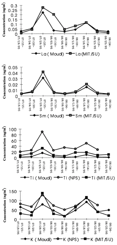
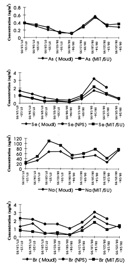
beginning on page 126. During the six-week sampling period, different events such as a dust episode, a hurricane influenced period, and a high pollution period were observed at the site which in turn caused broad variation of elemental concentrations. The dust event was observed from July 23 to July 26,1995; and a hurricane influenced the sampling site between August 2 and August 5. A pollution episode was observed from August 14 to August 18 associated with elevated concentration of sulfates. As expected, concentrations of crustal elements such as Al, Sc, Ti, Mn, Fe, and the Rare Earth Elements (REE) were high during the dust episode, and lower during the hurricane period because they were mostly washed out by rain. Elements released mostly from human activities such as As, Se, Br and Sb were higher during the pollution episode and were lower after the hurricane when the air was clean. Figures 2.4 and 2.5 show the time series distribution of selected elements.

Tables 2.5 and 2.6 show the average and standard deviations of size-fractionated UMn/MOUDI and CIT/MOUDI samples. The full data set for these samples is given in Appendix A beginning on page 137. The fraction size listed in the table is the lower limit of the particle diameter which was included in that fraction based on a criterion that 50% of particles at that size be in the next larger fraction. The fact that some of the elements have a standard deviation larger than their average value indicates a wide variation for that element's measured concentrations among the sample set. Data with no standard deviation listed are from a single measurement. The UMn/MOUDI sampler was attached to an inlet cyclone which removed coarse particles (John and Reischl, 1980) and it may have changed the

collecting efficiencies at the larger sizes. Because of limited knowledge of collection efficiencies of particles greater than 1.8 jim, only particles with an da less than 1.8 jim are included in Table 2.5. In the CIT/MOUDI samples, Zefluor filters were used to collect particles less than 0.056 gim. However, following the long irradiations, filter materials became brittle and some parts of them were not recovered. These samples are not included in Table 2.6.

Elements formed primarily by high-temperature anthropogenic activities, and as secondary aerosols such as As, Br, Cr, Sb, and Se show a maximum concentration at sub-micron sizes as shown in the UMn/MOUDI samples. Elements primarily formed by natural mechanical processes and from crustal materials such as Al, Fe, La, Mg, Mn, Na, Sc, Sm, and Ti have maximum concentrations at sizes larger than 1 m, and thus only the lower tail of their size distribution is seen in this data. The same trend was also found in CIT/MOUDI samples. Table 2.7 shows the analytical result of NPS/IMPROVE samples. These data are compared with the MIT/SU samples in the next section of this thesis.

Four 24-hour vapor phase Hg samples were collected during each week of the field operation at the eastern site. Atmospheric vapor and particulate phase Hg concentrations measured in this study compared well with values reported in the literature (Table 2.8). Because vapor phase Hg has an atmospheric lifetime of about one year, it is well mixed hemispherically. Therefore, its atmospheric concentrations do not vary as greatly as compared with the particulate phase, which has a lifetime on the order of several days. The average vapor phase concentration for the sampling period was 1.8 ng/m3 with a standard deviation of 0.6 ng/m3. As has been found previously (Olmez et al., 1996), there was essentially no correlation between the vapor and particulate phase measurements (r2 =0.077), and the vapor phase comprises the vast majority (98%) of the total atmospheric burden. The full data set for these samples is given in Appendix A on page 171.

Table 2.4. Summary statistics of MIT/SU 2.1 gm samples (ng/m3)

Geometric %

Element N Mean Median a Minimum Maximum

mean Observed Na 42 65 59 51 43 8.2 210 100 Mg 29 50 41 41 34 12 130 69 Al 38 139 63 65 205 1.1 920 90 CI 25 21 8.0 8.8 28 0.2 110 60 K 28 64 39 41 69 7.7 320 67 Sc 42 0.022 0.0093 0.012 0.029 0.0027 0.14 100 Ti 32 16 12 12 13 3.7 61 76 V 40 0.49 0.41 0.36 0.39 0.012 1.9 95 Cr 40 0.83 0.73 0.69 0.63 0.27 3.7 95 Mn 42 1.5 1.0 1.0 1.7 0.30 8.5 100 Fe 42 93 55 64 100 8.0 510 100 Co 42 0.15 0.13 0.12 0.10 0.018 0.56 100 Zn 42 11 8.0 6.0 11 0.2 42 100 Ga 6 0.30 0.19 0.20 0.34 0.056 0.98 14 As 42 0.30 0.29 0.25 0.19 0.054 0.77 100 Se 40 0.88 0.62 0.60 0.81 0.068 3.52 95 Br 41 0.82 0.44 0.51 0.87 0.086 3.90 98 Rb 3 0.45 0.44 0.44 0.16 0.33 0.56 7 Sr 11 2.4 2.0 1.9 1.5 0.37 5.6 26 Mo 16 0.13 0.099 0.10 0.15 0.041 0.67 38 Cd 24 0.094 0.075 0.073 0.068 0.011 0.29 57 In 22 0.0017 0.0017 0.0014 0.0011 0.00033 0.0036 52 Sb 38 0.33 0.24 0.25 0.26 0.020 1.37 90 Cs 20 0.032 0.029 0.023 0.024 0.0033 0.082 48 Ba 23 4.0 3.7 3.5 2.2 1.2 8.8 55 La 24 0.11 0.064 0.046 0.15 0.001 0.64 57 Ce 19 0.22 0.090 0.093 0.33 0.011 1.30 45 Nd 15 0.32 0.33 0.28 0.18 0.11 0.68 36 Sm 42 0.012 0.0043 0.0060 0.018 0.0006 0.089 100 Eu 23 0.009 0.0077 0.0070 0.0069 0.0011 0.027 55 Tb 13 0.006 0.0046 0.0047 0.0054 0.0009 0.022 31 Yb 23 0.011 0.011 0.010 0.0073 0.0040 0.031 55 Lu 10 0.0019 0.0021 0.0015 0.0011 0.00033 0.0038 24 Hf 6 0.0090 0.0073 0.0080 0.0051 0.0044 0.019 14 Ta 5 0.054 0.050 0.052 0.016 0.035 0.071 12 Au 10 0.0053 0.0055 0.0038 0.0034 0.00033 0.011 24 Hg 37 0.035 0.025 0.026 0.032 0.0077 0.17 88 Th 2 0.049 0.049 0.042 0.037 0.023 0.076 5 U 8 0.018 0.013 0.013 0.018 0.0058 0.060 19

L-, 1.00E+03 S8.00E+02 6.00E+02 A 4.00E+02

8

Concentration (nglm 3 ) M t~3l M M M £611/TLO 961LIlLO £6/L 1/LO £616 1/LO

96/1Z/LO £6/LZILO 96/6Z/LO£I

LILO

96/ZO/SO

£6tO/SO S600/180 96/90/S0 6/90/80 96/01/80 £6/Z1/80 96AIT/80 56/91/80 £6181/80 96/OZ/80 96/ZZ/80 96/t7Z/80

Concentration (nglm3) LA o 0 0

56/1/LO 961LIILO £6/61/L0 6/1IZ/ILO 6/EZ/ILO S61gZ/LO 6/LZ/ILO [6/6Z/L 6/1

EILO 96/ZO/80 56390180 96/90/80 56/80/80 £6/01/80 96/Z 1/SO 961V180 £6/t'1/80 96/91/80 6/8 1/80 96/0Z/80 96/1Z/80 16/1,80 Concentration (ng/m 3 ) + + + + 0 0 0 0 0 0 0 D 961511LO' 96/61/LO 96/11WL£66 IILO £611 ZILO

96/g2/LO 96/LZ/LO 96/6Z/LO £6/I

LILO 6/ ZO/80 £6/VO/SO £6190/80 £6/80/80 96/01/80 96/Z1/90 96/91/90 £6/8 1/80 56/OZ/SO 96/ZZ/80 96/t'S80 VI

o,

,

o]

°, ,,o]

L/_

II

96111LO 961611LO 6/IZILO £61/ZILO 561gZILO 961LZILO 6161Z/LO 56/1TL0 961Z0180 £q6/VO/SO £6/90/80 96190/80 96101/80 96/ZT/[8096/t

1/SO

96/91/805618

[180

Table 2.5. Average elemental concentrations (ng/m3) and standard deviations among the sample sets for each UMn/MOUDI size fraction. Size (mrn) < 0.056 0.056 0.098 0.175 0.32 0.56 1 Na 0.57 + 0.53 0.46 + 0.40 0.54 + 0.45 2.2 + 1.0 3.5 + 1.4 5.7 + 2.1 22 + 10 Mg 0.46 + 0.39 0.70 + 0.42 0.60 + 0.54 0.87 + 0.44 1.8 + 2.4 3.4 + 1.8 12 + 5 Al 0.91 + 1.01 1.1 + 0.7 2.8 + 5.1 13 + 31 2.2 + 2.3 19 + 24 53 + 46 C1 0.39 + 0.34 0.46 + 0.19 0.49 + 0.49 0.65 + 0.68 0.73 + 0.95 0.44 + 0.31 1.6 + 2.6 K 1.0 + 0.3 1.1 + 0.6 2.5 + 0.9 7.2 + 2.8 11 + 5 11 + 5 15 + 10 Sc 0.00005 0.00008 + 0.00009 0.0003 + 0.0004 0.0018 + 0.0029 0.0089 + 0.0092 Ti 0.03 0.38 0.19 + 0.22 0.22 + 0.15 0.64 + 0.20 0.82 + 1.01 3.0 + 2.9 V 0.032 + 0.027 0.005 0.021 0.057 + 0.082 0.12 + 0.06 0.11 + 0.06 0.10 + 0.08 Cr 0.8 + 1.1 0.30 + 0.10 0.08 + 0.10 0.23 + 0.32 0.23 + 0.41 0.39 + 0.52 0.18 + 0.16 Mn 0.10 + 0.13 0.021 + 0.020 0.007 + 0.008 0.039 + 0.037 0.11 + 0.10 0.27 + 0.16 0.59 + 0.42 Fe 4.1 + 5.0 0.92 0.78 + 0.28 2.8 + 1.0 2.8 + 3.5 9.5 + 10.0 28 + 26 Zn 0.53 + 0.55 0.22 + 0.17 0.09 + 0.09 0.55 + 0.35 0.90 + 0.56 1.7 + 2.3 0.83 + 0.47 As 0.0006 0.0012 + 0.0008 0.0079 + 0.0053 0.046 + 0.015 0.089 + 0.040 0.096 + 0.064 0.047 + 0.029 Se 0.0010 0.0062 + 0.0044 0.0056 + 0.0046 0.055 + 0.042 0.18 + 0.10 0.27 + 0.22 0.18 + 0.18 Br 0.0017 0.014 + 0.012 0.13 + 0.08 0.37 + 0.23 0.55 + 0.46 0.13 + 0.09 Mo 0.010 + 0.008 0.0036 + 0.0021 0.0034 + 0.0014 0.013 + 0.008 0.016 + 0.008 0.015 + 0.009 0.013 + 0.006 Cd 0.0004 0.0068 + 0.0039 0.0028 + 0.0007 0.005 + 0.003 0.011 + 0.013 0.007 + 0.007 0.008 + 0.009 In 0.00013 + 0.00002 0.00012 + 0.00005 0.00015 + 0.00006 0.00027 + 0.00006 0.00034 + 0.00020 0.00057 + 0.00048 0.00063 + 0.00038 Sb 0.05 + 0.03 0.06 + 0.05 0.06 + 0.04 0.09 + 0.02 0.13 + 0.07 0.13 + 0.08 0.11 + 0.06 Cs 0.0025 + 0.0008 0.0031 + 0.0025 0.0031 + 0.0018 0.0026 + 0.0009 0.0035 + 0.0015 0.0047 + 0.0028 0.0065 + 0.0035 Ba 0.28 + 0.30 0.19 + 0.22 0.13 + 0.14 0.18 + 0.12 0.20 + 0.16 0.24 + 0.16 0.76 + 0.44 La 0.00028 + 0.00014 0.00033 + 0.00027 0.00045 + 0.00023 0.00076 + 0.00077 0.0015 + 0.0015 0.008 + 0.012 0.038 + 0.037 Nd 0.02 + 0.01 0.02 + 0.02 0.02 + 0.01 0.05 + 0.03 0.10 + 0.11 0.20 + 0.25 0.043 + 0.031 Sm 0.00005 + 0.00003 0.00004 + 0.00003 0.00004 + 0.00003 0.00008 + 0.00007 0.00019 + 0.00021 0.0011 + 0.0018 0.0049 + 0.0053 Eu 0.0011 + 0.0008 0.0009 + 0.0005 0.0008 + 0.0006 0.0008 + 0.0002 0.0010 + 0.0003 0.0011 + 0.0010 0.0020 + 0.0011 Au 0.00008 + 0.00007 0.00029 + 0.00080 0.00008 + 0.00010 0.00008 + 0.00007 0.00008 + 0.00008 0.00023 + 0.00050 0.00018 + 0.00026 Hg 0.0010 + 0.0003 0.0007 + 0.0004 0.0013 + 0.0010 0.0012 + 0.0005 0.0014 + 0.0007 0.0012 + 0.0009 0.0022 + 0.0009 U 0.00039 0.00025 0.00059 + 0.00017 0.00091 + 0.00088 0.00087 + 0.00007 0.00066 + 0.00032

Table 2.6. Average elemental concentrations (ng/m3) and standard deviations among the sample sets for each CIT/MOUDI size fraction. Size (gim) 0.056 0.097 0.18 0.32 0.56 1 Na 1.1 + 0.7 3.8 + 1.6 7.4 + 3.2 8.9 + 1.8 15 + 9 76 + 68 Al 13 + 10 3.6 + 2.9 3.5 + 3.0 2.9 + 1.0 11 + 13 22 + 17 C1 0.6 + 0.3 1.5 + 0.9 3.2 + 3.5 9.0 + 5.1 22 + 18 11 + 12 Sc 0.0025 + 0.0026 0.0006 0.0020 + 0.0018 0.0007 + 0.0005 0.0028 + 0.0014 0.0029 + 0.0019 V 0.05 0.20 + 0.17 0.90 + 0.68 2.0 + 1.5 1.5 + 1.6 0.54 + 0.69 Mn 0.12 + 0.13 0.37 + 0.30 0.34 + 0.24 1.1 + 0.85 1.0 + 0.69 0.80 + 0.19 Fe 51 +41 23+21 26+23 33 +21 36 + 23 65 +32 Zn 3.0 + 3.7 1.9 + 2.5 3.1 + 3.3 5.8 + 6.6 5.8 + 4.4 3.6 + 1.5 As 0.009 + 0.005 0.019 + 0.009 0.035 + 0.027 0.035 + 0.018 0.016 + 0.015 0.014 + 0.008 Se 0.005 0.10 + 0.15 0.08 + 0.14 0.24 + 0.22 0.27 + 0.33 0.13 + 0.12 Br 0.014 + 0.008 0.21 + 0.13 0.48 + 0.38 0.49 + 0.22 0.48 + 0.45 0.08 + 0.08 Cd 0.011 + 0.005 0.01 + 0.02 0.04 + 0.03 0.05 + 0.05 0.02 + 0.02 0.05 + 0.06 Sb 0.043 + 0.045 0.14 + 0.06 0.26 + 0.09 0.36 + 0.11 0.46 + 0.14 0.49 + 0.13 Ba 2.4 1.3 + 0.3 3.0 + 0.7 3.6 3.4 + 1.9 4.9 + 1.3 La 0.007 + 0.009 0.0035 + 0.0025 0.018 + 0.015 0.042 + 0.049 0.048 + 0.024 0.106 + 0.076 Ce 0.015 + 0.002 0.04 + 0.02 0.08 + 0.08 0.08 + 0.05 0.07 + 0.04 Sm 0.0009 + 0.0011 0.0003 + 0.0002 0.0008 + 0.0006 0.0006 + 0.0002 0.0011 + 0.0006 0.0035 + 0.0022 Au* 0.10 + 0.07 0.21 + 0.18 0.36 + 0.23 0.52 + 0.26 0.51 + 0.25 0.64 + 0.36 * pg/m3

Table 2.7. Summary statistics of NPS/IMPROVE 2.4 gm samples (ng/m3_{) ( n=41 ).}

Element N Average a Median Geometric mean Min Max % Observed

Al 32 210 220 110 150 40 970 78 Si 39 380 420 220 260 97 1960 95 S 41 3200 2800 1900 2300 380 12400 100 K 41 82 37 76 76 30 210 100 Ca 39 62 46 52 49 10 210 95 Fe 41 80 99 40 47 7.2 460 100 Cu 40 2.1 2.0 1.5 1.6 0.5 10.6 98 Zn 41 6 3.7 5.5 5.1 1.2 20 100 Pb 38 2.9 1.2 2.5 2.6 1.1 5.3 93 Se 36 1.5 1.2 0.99 1.1 0.13 5.8 88 Br 41 2.0 0.8 1.9 1.8 0.5 4.5 100 SO4 41 9700 9100 5200 6500 1100 43000 100 NH4 41 1800 1350 1200 1300 61 4980 100

Table 2.8. Average vapor and particulate phase atmospheric mercury concentrations.

Vapor-phase Particulate

Location

(ng/m

)

(pg/Reference

(ng/m3) (pm3

North Pacific 1.77 < 2 Fitzgerald et al. 1991

Wisconsin 1.57 22 Fitzgerald et al. 1991

Tennessee 2.15 30 EPRI Report 1994

Nordic 2.5 - 2.8 60 Iverfeldt, 1991

Florida 1.64 1.5 - 8 Landing et al., 1994

New York 2.2 - 2.6 37- 62 Olmez et al., 1996