HAL Id: hal-01539481
https://hal.sorbonne-universite.fr/hal-01539481v2
Submitted on 7 Nov 2018
HAL is a multi-disciplinary open access
archive for the deposit and dissemination of
sci-entific research documents, whether they are
pub-lished or not. The documents may come from
teaching and research institutions in France or
abroad, or from public or private research centers.
L’archive ouverte pluridisciplinaire HAL, est
destinée au dépôt et à la diffusion de documents
scientifiques de niveau recherche, publiés ou non,
émanant des établissements d’enseignement et de
recherche français ou étrangers, des laboratoires
publics ou privés.
Meihui Gao, Bernardetta Addis, Mathieu Bouet, Stefano Secci
To cite this version:
Meihui Gao, Bernardetta Addis, Mathieu Bouet, Stefano Secci. Optimal Orchestration of Virtual
Net-work Functions. Computer NetNet-works, Elsevier, 2018, 142, pp.108-127. �10.1016/j.comnet.2018.06.006�.
�hal-01539481v2�
Optimal Orchestration of Virtual Network Functions
Meihui Gao
∗, Bernardetta Addis
∗, Mathieu Bouet
†, Stefano Secci
‡∗
Universit´e de Lorraine, CNRS, LORIA, F-54000 Nancy, France. Email: {meihui.gao,bernardetta.addis}@loria.fr
†Thales Communications & Security, France. Email: [email protected]
‡
Sorbonne Universit´e, CNRS, LIP6, F-75005 Paris, France. Email: [email protected]
Abstract—The emergence of Network Functions Virtualization (NFV) is bringing a set of novel algorithmic challenges in the op-eration of communication networks. NFV introduces volatility in the management of network functions, which can be dynamically orchestrated, i.e., placed, resized, etc. Virtual Network Functions (VNFs) can belong to VNF chains, where nodes in a chain can serve multiple demands coming from the network edges. In this paper, we formally define the VNF placement and routing (VNF-PR) problem, proposing a versatile linear programming formulation that is able to accommodate specific features and constraints of NFV infrastructures, and that is substantially different from existing virtual network embedding formulations in the state of the art. We also design a math-heuristic able to scale with multiple objectives and large instances. By extensive simulations, we draw conclusions on the trade-off achievable between classical traffic engineering (TE) and NFV infrastructure efficiency goals, evaluating both Internet access and Virtual Private Network (VPN) demands. We do also quantitatively compare the performance of our VNF-PR heuristic with the classical Virtual Network Embedding (VNE) approach proposed for NFV orchestration, showing the computational differences, and how our approach can provide a more stable and closer-to-optimum solution.
Index Terms—Network Functions Virtualization, VNF orches-tration, VNF chaining, VNF placement
I. INTRODUCTION
After about ten years of fundamental research on network virtualization and virtual network embedding, the virtualiza-tion of network funcvirtualiza-tions is becoming a reality thanks to huge investments being made by telecommunication providers, cloud providers and vendors.
The breaking point sits in 2012, when calls for experimen-tation and deployment of what was coined as “Network Func-tions Virtualization (NFV)” [2] lead to the creation of an NFV industry research group at the European Telecommunications Standards Institute (ETSI) [3]. Since then, applied researches and developments have accelerated investments, hence prelim-inary prototypes were demonstrated and deployed (leading to commercialization in some cases) since late 2014 [4].
With NFV, the attention of network virtualization research is now focusing on key aspects of NFV systems that were either not considered relevant or not conceived before industry effort at Standards Developing Organizations (SDOs). A central role is played by the NFV service chaining [5] provisioning, i.e., the problem of allowing a traffic flow passing through a pre-computed or dynamically computed list of VNF nodes, possibly accounting for the fact that VNF nodes can be placed
A preliminary version of this paper appeared in [1].
at, and migrated across, virtualization clusters as a function of demand assignment to existing VNF chains or sub-chains. Key aspects that are worth being mentioned (and often neglected in the proposed solution strategies) are the:
• ingress/egress bit-rate variations at VNFs, due to specific
VNF operations (such as compression as with a firewall function or an egress tunneling function, or such as decompression as in an ingress tunneling function);
• VNF processing and forwarding latency as an
orches-tration parameter. It can indeed be exponential with the traffic load on the VNF, or constant up to a maximum board if computation offloading solutions, such as direct memory access bypassing the hypervisor (as done with Intel/6WIND Data-Plane Development Kit [6]), or similar other ‘fastpath’ solutions are present.
We could not identify a work in the state of the art jointly taking these aspects all together into account. Furthermore, as summarized in Section II, most of the approaches rely on heuristic algorithms. Therefore, we propose a mathematical programming model integrating all of them and devise a method to find solutions for large size instances. A recent study [7] evaluates some of them highlighting that they may come at a “Revenue/Cost” ratio of 50%, i.e., twice as many resources were consumed than demands realized by heuristic approaches, which suggests that there is significant optimiza-tion potential to achieve in the area, despite the high number of research papers on VNF orchestration. In this paper, we focus on the problem modeling and optimization, proposing a mathematical formulation to solve the NFV MANagement and Orchestration (MANO) decision making to optimality under reasonable execution time targets.
ETSI is de-facto the reference SDO for the NFV high-level functional architecture specification. High-high-level means that its identified role is the specification of the main func-tional blocks, their architecture and inter-relationship, whose implementation elements could then be precisely addressed by other SDOs. ETSI specifies three components [8] for the NFV architecture: Virtual Network Functions (VNFs); NFV Infrastructure (NFVI), including the elements needed to run VNFs such as the hypervisor node and the virtualization clus-ters; MANO, handling the operations needed to run, migrate, optimize VNF nodes and chains, possibly in coordination with transport network orchestrators.
MANO procedures come therefore to support the economies of scale of NFV, so that physical NFVI virtualization resources (NFVI nodes) dedicated to NFV operations are used efficiently
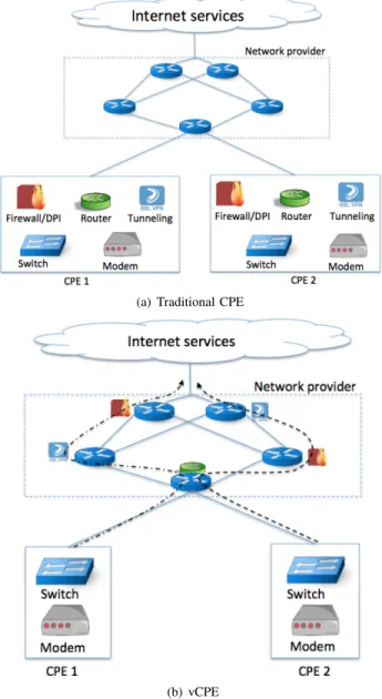
with respect to both NFVI operators and edge users. A promising NFV use-case [9] for carrier networks is the virtual Customer Premises Equipment (vCPE) that simplifies the CPE equipment by means of virtualized individual network func-tions placed at access and aggregation network locafunc-tions, as depicted in Fig. I. There are also other promising use-cases like the virtualization of the Evolved Packet Core (EPC) cluster in cellular core networks [10], [11], and the virtualization of cellular base stations [12].
(a) Traditional CPE
(b) vCPE
Fig. 1. Traditional Customer Premises Equipment (CPE) compared to
virtualized CPE (vCPE) with VNF chaining.
MANO operations are many and range from the placement and instantiation of VNFs to better meet user’s demands to the chaining and routing of VNF chains over a transport network disposing of multiple NFVI locations. Part of the orchestration decision can also be the configuration of the VNFs to share them among active demands, while meeting common Traffic Engineering (TE) objectives in IP transport networks as well as novel NFV efficiency goals such as the minimization of the number of VNF instances to install. In this context, the paper
contribution is as follows:
• we define and formulate via mathematical programming
the VNF Placement and Routing (VNF-PR) optimiza-tion problem, including compression/decompression con-straints and two forwarding latency regimes (with and without fastpath), under both TE and NFV objectives; our mathematical programming model is the first one in the literature taking into account explicitly all these key aspects together;
• we compare the VNF-PR approach to the legacy Virtual
Network Embedding (VNE) approach, qualitatively and quantitatively; to the best of our knowledge no other paper proposes such a comparison;
• we design a model tailored math-heuristic approach
al-lowing us to run experiments also for large instances of the problem within an acceptable execution time;
• we evaluate our solution by extensive simulations. We
draw considerations on NFV deployment strategies. The paper is organized as follows. Section II presents the state of the art on NFV orchestration. Section III describes the network model and the Mixed Integer Linear Programming (MILP) formulation. Analysis and discussion of optimization results are given in Section IV. Section V concludes the paper.
II. BACKGROUND
Network virtualization research was first driven by the convergence of computation, storage and network in cloud computing. A large number of works in the literature address the optimization of Virtual Machines (VM) placement with respect to, for example, server load balancing or energy sav-ing [13], [14]. Virtualizsav-ing the network between VMs is also a problem addressed in the area, defined as the Virtual Network Embedding (VNE) problem of mapping a set of logical graphs of interconnected VMs on a substrate graph [15].
In NFV, network functions that were once run by hardware-based middleboxes [16] are now meant to be virtualized as VNFs. VNFs can be chained together to provide a specific ser-vice, also known as service/VNF chaining. Service providers can deploy specific service chains to provide network service demands that requested by clients.
Preliminary works on NFV orchestration tend to solve the NFV orchestration problem as a VNE problem, which treats virtual network requests as logical graphs to be embedded into a substrate network. This is for example the case of [17]. VNFs are treated as normal VMs, mapped on a network of VM containers, which are interconnected via physical links that host logical links of virtual network demands. Similarly, authors in [18] propose a VNF chain placement that combines location-routing problems and VNE problems, solving first the placement and then the chaining. In [19] the authors decouple the legacy VNE problem into two embedding problems: VM embedding and service chain embedding, where a service chain is embedded on VMs, and each VM on physical servers. Each service chain has specific requirements as notably an end-to-end latency requirement. In [20] the authors consider specific constraints to guarantee the quality of service re-quirements in terms of forwarding latency and service chain
availability. An Integer Linear Programming (ILP) model is proposed to solve the resource cost optimization problem. In addition, to cope with large instances, a greedy algorithm based on sequential chain embedding is introduced for pro-viding near optimal solution in shorter execution time.
In its more general form, covering all the aspects of practical VNF operations, the placement and routing of VNFs does not directly match the classical VNE problem.In VNE, virtual network nodes need to be placed in an underlying physi-cal infrastructure. However, differently from VNE, in VNF placement and routing: (i) the demand is not a multipoint-to-multipoint network connection request, but a point-to-point source-destination flow routing demand, i.e., VNE introduces a superstructure unnecessary to represent the problem; (ii) the VNF chain can in general have a free or partial order, feature that cannot be easily represented with the VNE model perspective; and (iii) specific aspects of NFV such as for-warding latency behavior, ingress/egress bit-rate changes, and VNF/chain composition (i.e., sharing of nodes in the VNE terminology and selection among different node sizes) are not addressed in VNE. Their inclusion would further increase the VNE time complexity (for instance, in [21] forwarding latency is considered by adding ‘hidden nodes’ hence largely increas-ing the spatial and time complexities). In this sense, the VNF placement and routing problem is closer to a facility location problem, whereas VNE is closer to a mapping problem.
We argue in this paper that the appropriate way to deal with NFV MANO decision problems [22], [23] is to define the VNF Placement and Routing (VNF-PR) problem directly tailored to the NFV environment, for the sake of time complexity, modeling precision and practical usability. This is also the approach adopted by a few papers in the literature [24], [25], [26]. In [24] the authors consider the online orchestration of VNFs, modeling it as a scheduling problem of VNFs and proposing heuristics to scale with the online nature of the framework. In [25] the authors study a bi-criteria ap-proximation algorithm for the cost minimization objective function as well as for the nodes size constraints. In [26] the authors propose a formulation of the VNF placement and chaining problem and an ILP model to solve it. Additionally, to cope with large infrastructures, they introduce a binary search procedure for efficiently guiding the ILP solver towards feasible, near-optimal solutions. Different to [24], [25], [26], in this paper, we focus on providing a more generic formulation to the VNF placement and routing problem. Apart from chaining with VNF ordering guarantees, we also capture and investigate the practical feature of traffic flow compression and decompression that could be imposed by the VNFs along the traffic route.
A common approach is to rely on graph properties to find a better utilization of the limited resources while serving a larger set of demands. In [27] the specific Deep Packet Inspection (DPI) VNF node placement problem (without chaining) is targeted, with a formal definition of the problem and a greedy heuristic algorithm to solve it. In [28] the authors propose a heuristic to place and chain a maximum number of VNFs under capacity limitation; a linear programming approach is formulated to iterate the k-shortest paths computation for each
VNF chain and choose the one that satisfies the maximal length and number of reused VNFs. In comparison, our pro-posal considers not only the efficiency of resources utilization, but also the quality of service provisioning (for instance, the traffic forwarding latency). Moreover, we discuss the trade-off between resources efficiency goals and network traffic engineering goals.
Recently, game theoretic approaches are also considered: in [29] authors propose a heuristic based on routing games; in [30] authors propose a distributed dynamic pricing approach to allocate demands to already placed VNF instances, with convex congestion functions for both links and VNFs to control congestion.
Finally, the VNF placement and routing problem has also been addressed in specific contexts: wireless local area net-works [31] and optical netnet-works [32]. A comprehensive sur-vey on NFV resource allocation and chaining was recently published in [33].
Our paper takes inspiration from these early works, yet goes beyond being more generic and integrating in a mathematical programming model the specific features of NFV environ-ments mentioned in the introduction and formalized in the following.
III. NETWORKMODEL
We provide in the following a problem statement, its math-ematical programming formulation, and a description of its possible customization alternatives.
A. Problem statement
Definition Virtual Network Function Placement and Routing (VNF-PR) Problem
The network is represented by a graph G(N, A), where N is the set of switching nodes, and A represents the possible directional connections between nodes. The router i ∈ N and its associated NFVI cluster are represented by the same node; this choice allows to keep the size of the graph limited and
reduces the computational effort. We represent with Nv⊂ N
the set of nodes N disposing of NFVI server clusters. We consider a set of demands D, each demand k ∈ D is
characterized by a source ok, a destination tk, a nominal
bandwidth bk (statistically representative for demand k), and
a sequence of VNFs of different types, that must serve the demand (and therefore must be traversed by the demand). For each VNF a single VM is reserved, therefore we can equivalently speak of allocating a VM or a VNF on an NFVI node, meaning that we are reserving the necessary resources (e.g., CPU, RAM) to host a VM running a VNF. The VNF-PR optimization problem is to find:
• the optimal placement of VNF instances over NFVI
nodes;
• the optimal routing for demands and their assignment to
VNF node chains.
• subject to:
– link capacity constraints; – NFVI node capacity constraints;
– VNF forwarding latency constraints; – VNF node sharing constraints;
– VNF chain (total or partial) order for each demand. The optimization objective should contain both network-level and NFVI-network-level performance metrics. In our network model, we propose as network-level metric a classical TE metric, i.e., the maximum link utilization and as NFVI-level metric a measure of the overall allocated computing resources. Both objectives are - in a sequential way - minimized in the optimization model.
Furthermore, we assume that:
• Multiple VNF instances of the same type (i.e., same
functionality) can be allocated on the same node. Each
VNF instance can serve multiple demands1, but each
demand cannot split its flow on multiple VNF instances of the same type.
• The VNF computing resource consumption can be
ex-pressed in terms of live memory (e.g., RAM) and Com-puting Processing Units (CPUs), yet the model shall be versatile enough to integrate other computing resources.
• Latency introduced by a VNF instance can follow one
among the two following regimes (as represented in Fig. 2):
– Standard: VNFs buffer traffic at input and output virtual and physical network interfaces such that the forwarding latency can be considered as a convex piece-wise linear function of the aggregate bit-rate at the VNF, due to increased buffer utilization and packet loss as the bit-rate grows as shown in [6], [34]. This is the case of default VNFs functioning with standard kernel and hypervisor buffers and sockets.
– Fastpath: VNFs use optimally dimensioned and rel-atively small buffers, and decrease the number of times packets are copied in memory, so that the forwarding latency is constant up to a maximum aggregate bit-rate after which packets are dropped (e.g., this happens for Intel/6WIND DPDK fastpath solutions [6]).
Fig. 2 gives examples of forwarding latency profiles for the two cases.
• For each demand and NFVI node, only one
compres-sion/decompression VNF can be installed. This allows us to keep the execution time at acceptable levels, without reducing excessively the VNF placement alternatives. This assumption can be relaxed at the cost of working on an extended graph, and therefore increasing the com-putational time of the algorithm.
1this level of granularity allows to model the forwarding latency introduced
by VNF instances
TABLE I
PARAMETER NOTATIONS FOR BASE MODEL. Sets
N all nodes
Nv⊆ N nodes equipped with an NFVI cluster
A ⊆ N × N all arcs (links)
D demands
R resource types (CPU, RAM, ...)
F VNF types
Parameters network parameters
γij link capacity
Γir capacity of node i ∈ Nvin terms of resource r ∈ R
demand parameters
ok origin of demand k ∈ D
tk destination of demand k ∈ D
bk nominal bandwidth of demand k ∈ D
mkf 1 if demand k ∈ D requests VNF of type f ∈ F
skf order coefficient for VNF f requested by demand k
VNF/VM parameters
rrr demand of resource r ∈ R for a VM
cfi maximum number of instances of VNF f on node i2
TABLE II
VARIABLE NOTATIONS FOR BASE MODEL. Binary variables
xk
ij 1 if arc (i, j) is used by demand k ∈ D
zikf n 1 if demand k ∈ D uses the n-th instance of VNF
of type f ∈ F placed on node i ∈ Nv
yf ni 1 if the n-th instance of VNF of type f is assigned
to node i ∈ Nv
wfik 1 if demand k uses a VNF of type f on node i ∈ Nv
Continuous variables
U ≥ 0 maximum allowed link utilization
πik≥ 0 position of node i in the path used by demand k
0 1 2 3 4 5 6 0.0 0.5 1.0 1.5 2.0 VNF forwarding latency (ms)
normalized traffic load fastpath standard
Fig. 2. Example of VNF forwarding latency profiles.
B. Mathematical formulation
We first introduce a basic model that does not take into account latency limitations and compression/decompression features. The reason of this choice is twofold. First, it allows a clearer explanation of the model and a step by step intro-duction of the technicalities that allow us to keep the model
2the maximum number of instances of VNF type f on a node i is
limited by node capacity, therefore without loss of generality, we can set cfi = bminr∈RΓrrirrc
linear; we recall that already without these two features, the model is a combination of a network design and a facility location. Second, as the model proved to be difficult to solve at optimality using a state of the art solver, we design a sequential procedure to reduce the solution computational time. In particular, instead of solving the overall model from the beginning, we solve a sequence of problems where the model details (latency, compression/decompression) are added
step by step3. Therefore, this presentation allows to put in
evidence the peculiarities of each model component.
1) Basic VNF-PR model: Table I and II report the
mathe-matical notation used in the following Mixed Integer Linear Programming (MILP) that represents the basic formulation of the VNF-PR problem. We use four families of binary variables.The first family is used to represent the path used by each demand:
• xkij represents the per-demand link utilization for demand
k;
The other three families of binary variables are used to repre-sent the VNF instantiation and the assignment of demands to VNF instances. Each VNF instance is represented by a triple (i, f, n) the n-th instance of a VNF of type f on node i;
• yf ni represents the allocation of the instance n of a VNF
of type f on a node i;
• zikf n represents the assignment of a demand k to instance
n of a VNF of type f , multiple demands can be assigned to the same VNF instance;
• wikf represents the assignment of demand k to a VNF of
type f on node i, the specific instance is not indicated. This variable is introduced to simplify constraints (10). It can be removed using the equivalence with the sum of corresponding variables z (see constraints (9)).
The continuous variable U is used to represent the max-imum link utilization in the network, that is the maxmax-imum fraction of link capacity that is used by the current solution.
Continuous variable πik is used to represent the position of
node i in the path used to route demand k. This family of variables is necessary to impose (total or partial) order in the VNF chain. As mentioned before, we consider two objective functions:
• TE goal: minimize the maximum network link utilization:
min U (1)
• NFV goal: minimize number of cores (CPU) used by the
instantiated VNFs: minX i∈Nv X f ∈F X n∈1..cfi rrCP U y f n i (2)
The former objective allows taking into consideration the inherent fluctuations related to Internet traffic and therefore minimizing the risk of sudden bottleneck on network links in the case bandwidth demands deviate from the expected values. Therefore, minimizing the fraction of link capacity that can be used, indirectly allows controlling the network congestion. The latter assumes the fact that today the first
3see Subsection III-C for a detailed description of the procedure
modular cost in virtualization servers, especially in terms of energy consumption and monetary cost, is the CPU. Since in common VM templates, the RAM resource is positively correlated to the CPU resource, considering CPU as reference cost indicator can indirectly imply also the consideration of the RAM consumption. We now present the constraints.
Single path flow balance constraints:
X j:(i,j)∈A xkij− X j:(j,i)∈A xkji= 1 if i = ok −1 if i = tk 0 otherwise ∀k ∈ D, ∀i ∈ N (3) Utilization rate constraints:
X
k∈D
bkxkij ≤ U γij ∀(i, j) ∈ A (4)
Node resource capacity (VNF utilization) constraints: X f ∈F X n∈1..cfi rrry f n i ≤ Γir ∀i ∈ Nv (5)
Each demand uses exactly one VNF of each required type: X
i∈Nv
X
n∈1..cfi
zikf n= 1 ∀k ∈ D, f ∈ F : mkf= 1 (6)
Constraints (7)-(9) are consistency constraints among binary variables. A VNF can be used only if present, for a given node:
zf nik ≤ yf ni ∀k ∈ D, i ∈ Nv, f ∈ F, n ∈ 1..cfi (7)
If a demand does not pass by a VNF, it cannot use it:
zikf n≤ X
j:(j,i)∈A
xkji ∀k ∈ D, i ∈ Nv, f ∈ F : m
f
k = 1 (8)
Auxiliary variables for ensuring consistency: X
n∈1..cfi
zikf n= wfik, ∀k ∈ D, i ∈ Nv, f ∈ F (9)
Finally, we introduce constraints to avoid unfeasible routing and to impose the VNF chain order:
Preventing the formation of isolated cycles:
πjk≥ πik+ xkij− |Nv|(1 − x
k
ij) ∀k ∈ D, (i, j) ∈ A (10)
Imposing an order for virtual functions:
πjk≥ πik− (|Nv| + 1)(2 − wf1 ik− w f2 ik) ∀k ∈ D, ∀i, j ∈ Nv, f1, f2∈ F : s f2 k ≥ s f1 k (11)
If we consider flow balance constraints (3) and link capacity constraints (4), for each demand, a selection of arcs forming a path plus an isolated cycle can be a feasible solution. In pure routing problems, these solutions are equivalent to the solution where routing variables along the cycle are removed and only the one along the path are kept. In fact, both constraints (3) and constraints (4) will be valid for this new solution. Our problem integrates routing features within a facility location problem, therefore such solutions cannot always be transformed in a simple path simply removing the cycle. In fact, if a facility (VNF) used by the demand is located on the cycle, removing the cycle will produce an unfeasible solution. Therefore, it is
TABLE III
NOTATIONS TO MODEL FORWARDING LATENCY. Parameters
L maximum allowed latency for a demand
λij latency introduced by link (i, j) ∈ A
standardlatency model
gfj(b) j-th component of the linearized latency function
for VNF f and aggregated bandwidth b
ng number of piece-wise components of lin. latency function
fastpathlatency model
¯
lf latency introduced by VNF f
Bfmax maximum allowed bandwidth to traverse VNF f
Variables
lfik≥ 0 latency that demand k ∈ D incurs using VNF f
on node i of type f ∈ F hosted by node i ∈ Nv
necessary to remove such solutions directly in the model, to this aim we introduced constraints (10), inspired by traveling salesman problems tour elimination constraints [35]. Variable
πik represents the order of node i along the path serving
demand k, therefore if arc (i, j) exists, then πjk will be at
least πik plus 1. On the other side, if arc (i, j) does not
exist (xkij = 0) then the constraint is not active: πik is always
smaller than |Nv|, as a path can contain at most all the nodes in
the graph. In this way, only solutions containing simple paths are allowed. These variables are also used in Equation (11) to allow imposing an order on VNFs along the route of a demand
k. They impose that if demand k uses VNF f1located on node
i and its VNF successor f2(sf2
k ≥ s
f1
k ) that is located on node
j, then in the routing path of demand k node i must be precede node j.
2) VNF forwarding latency: We impose that for each
demand k ∈ D a maximum latency L is allowed, to guarantee some level of Quality of Service (QoS). Latency depends on two components: link latency, represented by a parameter λij for each arc (i, j), and VNF latency. VNF latency depends on the used model of latency (standard or fastpath). To keep the notation as uniform as possible, we introduce an additional
variable lfik to represent the latency experienced by demand
k traversing VNF f located on node i. Therefore we get a set of constraints common to both models limiting the overall latency: X (i,j)∈A λijxkij+ X i∈Nv X f ∈F lfik≤ L ∀k ∈ D (12)
A set of constraints depending on the chosen latency model
allows to calculate the value of variable likf.
• Standard: the latency introduced on demand k for using
VNF f depends on the overall traffic traversing the VNF
(its own and the one of others demands). Let us call gjf(·)
the j-th component of the piece-wise linearization of the latency function for VNF of type f , then we get:
lfik≥ gfj(X
d∈D
bkzidf n) − L(1 − zf nik)
∀k ∈ D, i ∈ Nv, f ∈ F, n ∈ 1..cfi, j ∈ 1..ng (13)
We can observe that constraint (13) is active only when the demand uses instance n of VNF f on node i
TABLE IV
NOTATIONS TO MODEL BIT-RATE VARIATIONS. Sets
Na access nodes
Na0 duplication of access nodes, where demands are located
Parameters
µf compression/decompression factor for VNF f ∈ F
bmin
k minimal bandwidth of demand k ∈ D
bmax
k maximal bandwidth of demand k ∈ D
Mi maximum traffic volume that can be switched by node i
Variables
φkij≥ 0 flow for demand k ∈ D on arc (i, j)
ψikf n≥ 0 flow for demand k ∈ D entering node i
and using instance n of VNF f ∈ F
(zikf n = 1). Otherwise, as overall latency is limited by
L (constraint (12)), any term gjf(·) must be smaller than
L, and therefore, the constraint is a redundant constraint
(lik ≥ 0). We can observe that, even if in the standard
latency model there is no theoretical limit on the allowed bandwidth, constraint (12) – limiting the overall latency for a single demand (VNFs forwarding latency plus propagation delay) – imposes an implicit limit on the maximum attainable bandwidth for a single VNF.
• Fastpath: the latency is fixed, but a limit in the total traffic
that a VNF can support is imposed. Therefore we get the following two sets of constraints:
lfik= ¯lf ∀k ∈ D, i ∈ Nv, f ∈ F (14) X k∈D bkzikf n≤ Bf max ∀i ∈ Nv, f ∈ F, n ∈ 1..c f i (15)
We can observe that constraints (14) can be substituted directly in constraints (12). Constraints (15) impose that the total bandwidth traversing the n-th VNF instance of type f on node i is limited by the maximum amount of bandwidth that the VNF instance can support before re-jecting a demand. Therefore, in our solutions no demand is discarded due to the fastpath mechanism.
3) Bit-rate compression/decompression: To introduce the
possibility of compressing/decompressing flows for some VNFs, we need some modifications to our model description.
We introduce a compression/decompression parameter µf for
each type of VNFs, µf > 1 means that a decompression
is performed by VNF f . When a demand pass through a
VNF with µf 6= 1, its bandwidth changes, therefore knowing
just the routing (x variables) is not enough to determine the overall flow along an arc. For this reason we introduce
variable φk
ij that represents explicitly the flow on arc (i, j)
for demand k. Another consequence is that the classical flow balance equations are not anymore valid. To extend the model without introducing an excess of complexity, we work under the assumption that given a node i, and a demand k, such demand uses at most a VNF f with a factor of
compression/decompression (µf6= 1).
We work on an extended graph to distinguish between access nodes (origin/destination nodes) and NFVI nodes (re-mind that with the basic model we collapsed NFVI nodes
original graph extended graph
i
j
i’
i
j
Fig. 3. Duplication of an access node i.
on router nodes). Each access node i is duplicated in a node
i0 as shown in Fig. 3. Arc (i, i0) will be added and all arcs
(i, j) originating from access node i will be transformed in
arcs (i0, j). Therefore, the routing functionality is on node
i and the NFVI functionality can be allocated on node i0.
Furthermore, we add variable φf nik, that represents the flow of
demand k entering node i and using the instance n of the VNF of type f . If a demand passes through a VNF with a factor of
compression/decompression µf, then the out-flow of the node
is proportional to the in-flow: X j∈N :(i,j)∈A φkij = µf X j∈N :(j,i)∈A φkji or equivalently: X j∈N :(i,j)∈A φkij− X j∈N :(j,i)∈A φkji= X j∈N :(j,i)∈A (µf− 1)φk ji
This equation is valid only if demand k uses an instance n of VNF f on given node i (remind that latency depends on the bandwidth passing throw a single instance). Therefore, to obtain a valid equation, we have to write:
X j∈N :(i,j)∈A φkij− X j∈N :(j,i)∈A φkji= X j∈N :(j,i)∈A φkji X n∈1..cfi (µf− 1)zikf n when P n∈1..cfi(µf − 1)z f n
ik = 0 the constraint states that
the in-flow and out-flow are the same, that is, if no VNF is traversed, the flow remains unchanged. The same result
is obtained for all VNF f such that µf = 1 (no
compres-sion/decompression). To the aim of linearizing this constraint,
we introduced variable ψikf n (still non-linear representation):
ψikf n= ( X
j∈N :(j,i)∈A
φkji)zikf n
The constraints can be linearized using Equations (20)-(22),
with the parameter Miequal toP
(j,i)∈Aγji, which represents
the maximum quantity of flow that can enter node i. If
(µf− 1)zikf n= 1 then ψikf n representing the flow of demand k
entering node i and passing through the instance n of the VNF f (constraint (20)-(21)), otherwise it is zero (constraint (22)). It is now possible to present the new constraints that must be
added to the basic VNF-PR model: Flow balance for access nodes: P j∈N :(i,j)∈A φk ij− P j∈N :(j,i)∈A φk ji= = bk if i = o k 0 otherwise −bk Q f ∈F :mfk=1 µf if i = tk ∀k ∈ D, i ∈ Na (16) Flow and compression/decompression balance for NFVI nodes and for each demand:
X j∈N :(i,j)∈A φkij− X j∈N :(j,i)∈A φkji= X f ∈F,n∈1..cfi (µf− 1)ψikf n ∀k ∈ D, i ∈ Nv (17)
Coherence between path and flow variables:
φkij ≤ bmax k x k ij ∀k ∈ D, (i, j) ∈ A (18) φkij≥ bmin k x k ij ∀k ∈ D, (i, j) ∈ A (19)
VNF compression/decompression linearization constraints:
ψikf n≤ P j∈N :(j,i)∈A φkji+ Mi(1 − zf nik) ∀k ∈ D, i ∈ Nv, f ∈ F, n ∈ 1..cfi (20) ψikf n≥ P j∈N :(j,i)∈A φkji+ Mi(1 − zf nik) ∀k ∈ D, i ∈ Nv, f ∈ F, n ∈ 1..cfi (21) ψikf n≤ Mizikf n ∀k ∈ D, i ∈ Nv, f ∈ F, n ∈ 1..cfi (22)
One compression/decompression VNF per node and demand: X
f ∈F
X
n∈1..cfi:µf6=1
zikf n≤ 1 ∀k ∈ D, ∀i ∈ Nv (23)
Eq. (16) represents the flow balance for the access nodes. At destination node the quantity of flows is set equal to the demand multiplied for all factors of compression of all the demanded VNFs. Eq. (17) represents the flow balance for a given node that has the possibility of hosting VNFs (NFVI). Eq. (18)-(19) allow to connect variables x and φ, in such a way that only and only if arc (i, j) is used by demand k,
that is xkij = 1, then variable φ can be different from zero.
As the demand passes through VNF that can compress or decompress the flow, then we can determine upper and lower
bound for the demand that are: bmaxk = bkQf ∈F :µf≥1 and
bmink = bkQ
f ∈F :µf≤1
4. Variables x are still necessary to
impose the isolated cycles elimination and the order in the VNF chain. The utilization rate constraints must be modified as follows:
X
k∈D
φkij ≤ U γij ∀(i, j) ∈ A (24)
4To avoid these parameters being zero when does not exist any VNF with
µf ≥ 1 (only decompression), and µf ≤ 1, respectively, the calculation of
the parameter can be modified in bmax
k = bkmax{1,Qf ∈F :µf≥1} and
bmink = bkmin{1, max{0,
Q
TABLE V
APPLICABLE CONSTRAINTS TOVNF-PRPROBLEM VARIATIONS. Constraints
Features routing/location latency profile bit-rate
basic (3), (4), (5)-(11)
basic-lat (3), (4), (5)-(11) (12), [(13) vs (14)-(15)]
basic-lat-cd (3), (24), (5)-(11) (12), [(13) vs (14)-(15)] (16)-(23)
To take into account the combined effect of compres-sion/decompression and VNF latency some modification are needed.
For the standard model, constraints (13) are modified as follows:
likf ≥ gfj(P
d∈D
ψf nid) − L(1 − zikf n)
∀k ∈ D, i ∈ Nv, f ∈ F, n ∈ 1..cfi, j ∈ 1..ng (25)
For the fastpath model, constraints (15) are modified as follows: X d∈D ψidf n≤ Bf max ∀i ∈ Nv, f ∈ F, n ∈ 1..c f i (26)
In Table V we summarize the different models. In the first column a short name is used to refer to each model, in the second column constraints necessary to model routing, loca-tion and resource capacity are reported. In the third and forth columns we report latency and compression/decompression constraints.
C. Multi-objective math-heuristic resolution
We face a multi-objective problem: minimizing the maxi-mum link utilization, which reflects the ISP-oriented vision to improve the user quality of experience (strictly related to link congestion, especially for real-time services) and minimizing the virtualization infrastructure cost evaluated as the number of required CPUs at the NFVI level, which reflects the aims of the NFVI provider. Such a multi-objective approach makes especially sense when the NFVI provider is a different entity than the ISP. These two objectives are in competition; in fact, to obtain a low utilization, a large number of VNFs must be allocated.
We decided to prioritize the objectives: first we minimize the maximal link utilization (U ), and then the NFV cost (total number of used CPU). We refer to this as the TE-NFV objective. In practice, we perform a first optimization step to find the best solution accordingly to maximal link utilization
(U?), and then, keeping the best value found in the first step as
a parameter (i.e. adding the constraint U ≤ U?), we minimize
the second objective (NFV cost). In fact, for a given optimal value of the first step, different possible configurations are available to the second step, and a large primary cost reduction can be achieved by this second step without losing with respect to the primary objective (maximum link utilization).
In order to understand the impact of imposing a maximal link utilization constraint on the NFV cost, we decided to study the sensitivity of the second step of optimization on the
opti-mal value U?. Therefore, we re-optimize the second objective
relaxing the constraint on the maximum link utilization by a
parameter α, i.e. we used constraint U ≤ α + U? instead of
U ≤ U?. We increase α step by step, until the value of the
NFV cost does not reduce anymore. This value corresponds to first minimize the NFV cost and then the maximum link utilization cost (NFV-TE).
From preliminary tests, we observed that optimizing the complete model is very expensive, and that computational time can be significantly reduced performing a sequence of optimization starting from a basic model to the complete one. The result of each step is used as a starting point for the following one, a so-called warm-start, that allows to reduce computational time and/or produce better solutions or gaps (when optimization is stopped before reaching the optimal solution). To be more precise, the sequence of models we optimize is first the basic one (only demand routing, VNF location and capacities are considered), then basic-lat (basic-latency is added) and finally basic-basic-lat-cd (basic-latency and compression/decompression are added), see Section III and Table V for the complete description of the models and equations involved.
The most challenging model from an optimization point of view is the last one, basic-lat-cd. For this reason, we need to provide a feasible starting solution (warm start) for this step. To this aim, the previous step, optimizing basic-lat model, must be done with some slightly modification. The compression/decompression feature changes the quantity of flow that traverses the graph, therefore to guarantee that the solution of the second step is feasible for the last one, it is necessary to route a worst case quantity of flow, given by the case that all the VNFs with decompression are already applied
to the demand flow5.
The NFV objective function results to be computationally more challenging than the TE one. Therefore, for obtaining the optimal solution of the NFV goal, a bisection procedure is used on the number of allocated VNFs/VMs to guarantee solution optimality, even when in a single step the solver is not able to guarantee it: that is, at each bisection step, if a feasible solution is found, the number of VNF/VM is divided by two, and if no feasible solution exists then it is doubled. From numerical experiments, we observed that, for our problem, determining that an instance is unfeasible (fixing a maximum number of VNF instances) using the TE objective is computationally less challenging than solving to optimality the model using the NFV objective function. For this reason, the speed up obtained using the bisection procedure allows us to solve to optimality, or obtain a solution with a small gap on a larger number of instances than solving directly the NFV objective problem.
D. Further model refinements
The model we provided above can be possibly refined and customized to meet specific requirements. We list in the following the possible variants as well as the corresponding modeling variations.
5Of course, this worst case can be improved considering the order of VNFs,
• VNF affinity and anti-affinity rules: due to the privacy, reliability or other reasons, a provider may want impose rules on the placement of certain types of VNF: be placed or not placed on certain servers, be grouped or not grouped together, etc. Such specific VNF placement rules are called affinity and/or anti-affinity rules [36]. To extend our model to take them into account, the simplest way is to introduce a new variable representing the presence of a certain type of VNF f on a given node i (we remind the reader that our model allows to have multiple copies of the same type of VNF on the same node). Let us call
this variable vfi, it will be equal to one if a VNF of type
f is located on node i. To make these variables consistent
with already defined variables yf ni , we need to add:
X
n∈1..cfi
ynfi ≤ cfivfi ∀i ∈ Nv, f ∈ F
More precisely, common affinity/anti-affinity rules are: – VNF-VNF affinity rules: if two VNFs communicate
frequently and should share a host node, we may want to keep the VNFs together in order to reduce traffic across the networks and improve the traffic
efficiency. Let AffVVf1f2 be a parameter equal to
one if f1 and f2 should share the same node. Then:
vf1
i = v
f2
i ∀(f1, f2) : AffVVf1f2 = 1
– VNF-Server affinity rules: certain intrusion preven-tion VNFs should reside in the network edges to guard against worms, viruses, denial-of-service
(DoS) traffic and directed attacks. Let AffVSfi be
a parameter equal to one if f should be installed on i. Then:
vif= 1 ∀(i, f ) : AffVSfi = 1
or restricted to a subset of nodes S ∈ Nv: X
i∈S
vif = 1 ∀(i, f ) : AffVSfi = 1
– VNF-VNF anti-affinity rules: it may be required to install multiple instances of the same VNF onto multiple servers in order to improve VNF reliability
against failures. Let AAfff be the anti-affinity
pa-rameter; we then impose that at least nbM in nodes host the VNF:
X
n∈Ns
vif ≥ nbM in ∀f : AAfff = 1
if different VNFs cannot be co-located, let
AAffVVf1f2 be the anti-affinity parameter and
im-pose:
vf1
i + v
f2
i ≤ 1 ∀(f1, f2) : AAffVVf1f2= 1
– VNF-Server anti-affinity rules: it may be required to avoid resource-hungry VNFs residing in certain
cost-critical servers. Let AAffVSfi be the anti-affinity
parameter and impose:
vfi = 0 ∀(i, f ) : AAffVSfi = 1
We can observe that all the constraints that set some variables to one or zero, just reduce the number of variables; therefore we can expect that such constraints do not increase the computing time. A slightly different condition can be imposed for sharing a VNF among different demands; we refer to that as VNF isolation.
• VNF isolation: if the same VNF cannot be shared between
two specific demands, we can add constraints to impose this condition. It is sufficient to introduce an
incompati-bility parameter inck1k2, equal to one if demand k1must
be isolated from demand k2; then we need to add:
zikf n
1+ z
f n
ik2 ≤ 1 ∀i ∈ Nv, f ∈ F,
n ∈ 1..cfi, k1, k2∈ D
• Multiple comp./dec. VNFs per NFVI node: to make the
presentation simpler, we assumed that in each NFVI node there is at most one VNF that can compress/decompress
a flow, i.e. with a factor of compression µf 6= 1. This
assumption can be relaxed using an extended graph in
which each node that can host a VNF (Nv) is expanded
in multiple copies, one for each type of VNF that can be allocated in the node. Otherwise, we can represent all possible combinations of different VNFs allocated to the same node, and adding additional binary variables to represent which combination is chosen.
• VNF partial chain ordering: we can observe that partial
order can be imposed with a the same form of constraints used for total ordering (11), just limiting their number to existing precedence conditions. It is sufficient to in-troduce a constraint for each couple of VNFs that has a precedence relation. More formally, for each demand
k, we can introduce a directed acyclic graph Ok(Vk, Pk),
where nodes V represent the set of VNFs that must serve
the demand (V = {i ∈ F : mfk = 1}), and arcs P
represent the order relation between such VNFs, that is an arc (i, j) ∈ P if VNF j must be used after VNF i. Then, constraints (11) can be rewritten as:
πjk≥ πik− (|Nv| + 1)(2 − wf1
ik− w
f2
ik)
∀k ∈ D, ∀i, j ∈ Nv, f1, f2∈ Vk : (f1, f2) ∈ Pk
• Additional computing constraints: it can be easily
in-cluded by tuning existing parameters, as far as computing resource requests can be expressed in an additive way (e.g., for storage).
• Load balancing: in the current model, each demand can
use a single VNF for each type. The model can be extended to allow per-VNF load balancing. If the load balancing is local to an NFVI node , the change in the model is small, in fact it is simply necessary to have some continuous variables taking into account the quantity of demand associated to each VNF. If the load balancing can be between different clusters, then it is necessary to extend the model allowing multiple paths for each demand. However such an extension is expected to largely increase the execution time.
• Different VM templates: for the sake of simplicity,
one-to-one correspondence between VNF and VM templates (single template). Nevertheless, multiple VM templates can be considered in the model at the price of increasing of one dimension/index all variables indexed on the VNF identifiers.
• Core router as a VNF: if the core routing function is
also virtualized, i.e., if the NFVI node and the network router can be considered as a single physical node that runs the core routing function, processing the aggregate traffic independently of the demand, as a VNF, then we need to add a term proportional to InFlow plus OutFlow to (5): X k∈D X f ∈F X n∈1..cfi rrryif n +X k∈D X j:(i,j)∈A bkxkij +X k∈D X j:(j,i)∈A bkxkji≤ Γir ∀i ∈ Nv, r ∈ R
If bit-rate compression/decompression is considered, con-straint (5) must be modified as follows:
X k∈D X f ∈F X n∈1..cfi rrryf ni +X k∈D X j:(i,j)∈A φkij +X k∈D X j:(j,i)∈A φkji≤ Γir ∀i ∈ Nv, r ∈ R IV. RESULTS
Computational results are divided in two main parts: first, in Section IV-A, we show results using our VNF-PR algorithm under different case-study choices of demand distribution and different VNF forwarding latency models and values. Then, in Section IV-B, we present comparison results between our VNF-PR algorithm and a VNE algorithm.
A. Results of VNF-PR algorithm under different case-studies and different VNF forwarding latency profiles
In this section, we report experiments on our VNF-PR model and algorithm under different scenarios. We first present the parameter setting and then the analysis of the results.
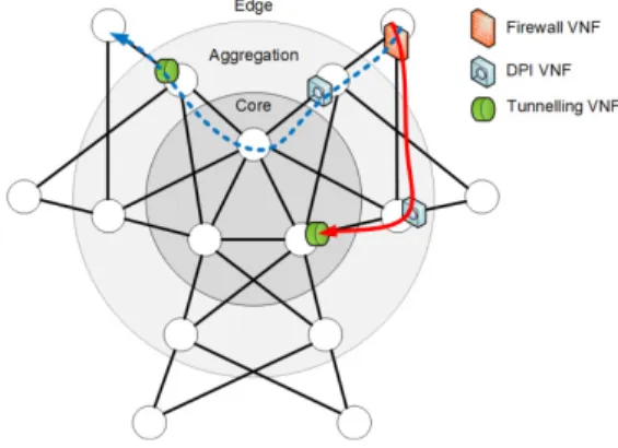
1) Test settings: We adopt the three-tier topology
repre-sented in Fig. 4 for computational evaluation. Each edge node is connected to two aggregation nodes, each aggregation node is connected to two core nodes, and core nodes are fully meshed. We believe that this topology gives a good abstraction to represent the current vision on NFV deployment strategies: mobile edge facilities are represented by edge nodes, point-of-presence by aggregation nodes and data-centers by core nodes. Furthermore, the highly symmetric graph topology produces two main effects: it allows to better analyze the VNF distribution and the effects of latency limits and, on the other hand, produce a very challenging instance for the optimization phase, allowing to test the model in a stressful
condition. As for the VNFs, we consider three VNF template types per traffic demand: one with a compression behavior, one with a decompression behavior and a third with no compression/decompression. For the sake of illustration, we name each of these templates with a realistic VNF type name: a ‘Firewall’ VNF for the compression (as it blocks part of the incoming traffic/packets), a ‘Deep Packet Inspection (DPI)’ VNF for the case with no compression, i.e., decompression, and a ‘Tunneling ingress VNF’ for the decompression (as headers are added to packet in the entry end-point). For the latter VNF, the assumption we do is that the egress tunneling is done elsewhere in the Internet or in the access border side. We considered a strict order for the VNFs chain: Firewall VNF first, then DPI VNF, and finally Tunneling ingress VNF. Each VNF instance has to reserve its own VM, and we consider one single VM template requiring 1 CPU and 16 GB of RAM.
Fig. 4. Adopted network topology and VNF-PR solution example. Table VI presents the evaluation settings of the network resources. NFVI nodes are dimensioned with an increasing capacity from edge to core: 3 CPUs and 40 GB RAM at each edge node, 5 CPUs and 80 GB RAM at each aggregation node and 10 CPUs and 160 GB RAM at core nodes. The physical links are also dimensioned with different capacity to represent realistic settings: the aggregation links are dimensioned so that there is a risk of link saturation (i.e. link utilization higher than 100%) if the traffic distribution is not optimized, while the core links are dimensioned such that there is a very low bottleneck risk. Link latencies are set as follows to cope for the different geographical scopes: 1ms for edge links, 3ms for aggregation links, and 5ms for core links.
TABLE VI
TEST SETTINGS OF NETWORK RESOURCES. NFVI node settings
NFVI node CPU unit RAM (GB)
Edge nodes 3 40
Aggregation nodes 5 80
core nodes nodes 10 160
Physical link settings
Physical link Bandwidth Latency (ms)
Edge links 1 1
Aggregation links 0.5 3
core nodes links 1 5
demand distribution: Internet and Virtual Private Network (VPN). In the Internet case-study (e.g., the flow in red on Fig. 4), the traffic demands are sent by each edge node (e.g., end user) to each core node (e.g., data center), and from each core node to reach each edge node, which means that in this case both edge nodes and core nodes are access nodes (i.e., where demands are generated); while under VPN case-study (e.g., the flow in blue on Fig. 4), the edge nodes send traffic requests to each other, which means that the set of edge nodes corresponds to the set of access nodes. The total number of traffic demands is different for the two case-studies (36 for Internet and 30 for VPN), but we kept constant the average total traffic volume (sum of demands) in the network for the sake of comparison. As shown in Table VII, the demands are randomly generated with uniform distribution of the required bandwidth volume in a given interval [a, b], in such a way that edge demands cannot create any bottleneck at the edge links, i.e., a = 0.1 and b = 0.14 in the Internet case-study, a = 0.13 and b = 0.17 in the VPN case-study. These values allow us to keep the total traffic volume at the same level for the two case-studies. In order to have more significant results than one single demand instance, we generate 10 random demand instances for each case-study.
TABLE VII
TEST SETTINGS OF TRAFFIC DEMANDS.
Study-case |D| a b Averaged total amount of
traffic volume
Internet 36 0.1 0.14 |D| ∗b−a
2 = 4.5
VPN 30 0.13 0.17 |D| ∗b−a
2 = 4.5
We run tests for both Internet and VPN case-studies under standard as well as fastpath latency profiles, VNF processing latencies being set as in Fig. 2. The two profiles differ for their behaviors with respect to the bandwidth: fastpath has a fixed latency and it rejects demands beyond a given threshold, while the standard profile can accept a larger amount of demands at the cost of a larger latency. For both profiles, the same end-to-end latency is assigned to the bandwidth corresponding to the fastpath threshold. This allows to better compare the behavior of the two profiles. With fastpath we expect to aggregate demands up to the threshold (in the limits of the granularity of the demands and the routing possibilities), whereas with the standard profile we expect that a larger latency can be accepted (as long as we stay in the overall latency demand threshold) to reduce the number of VNF instances. In addition, we consider two levels of end-to-end latency bound (L): the strict and loose values (15ms and 20ms, resp.). To be precise, we run tests with both strict and loose latency bounds for the following combinations of scenarios:
• TE goal and TE-NFV goal both with:
– Internet demand profile: ∗ standard forwarding regime ∗ fastpath forwarding regime – VPN demand profile
∗ standard forwarding regime ∗ fastpath forwarding regime
For a total of 16 different cases (each of them repeated for 10 random generated demand instances).
The model is implemented and solved using AMPL and CPLEX 12.6.3.0. The execution time is limited to 600s for each basic TE optimization phase (i.e., model basic and lat) and 800s for the complete TE phase (namely model basic-lat-cd), as well as for each step of the dichotomy of the NFV optimization phase.
2) General observations: In this section, we introduce
general considerations from a computational point of view, discussing the quality of the results in terms of optimality and gap of the solutions. In Section IV-A3 to IV-A6, we provide detailed analysis of the structure and properties of the solution in terms of network and system indicators.
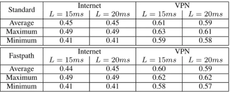
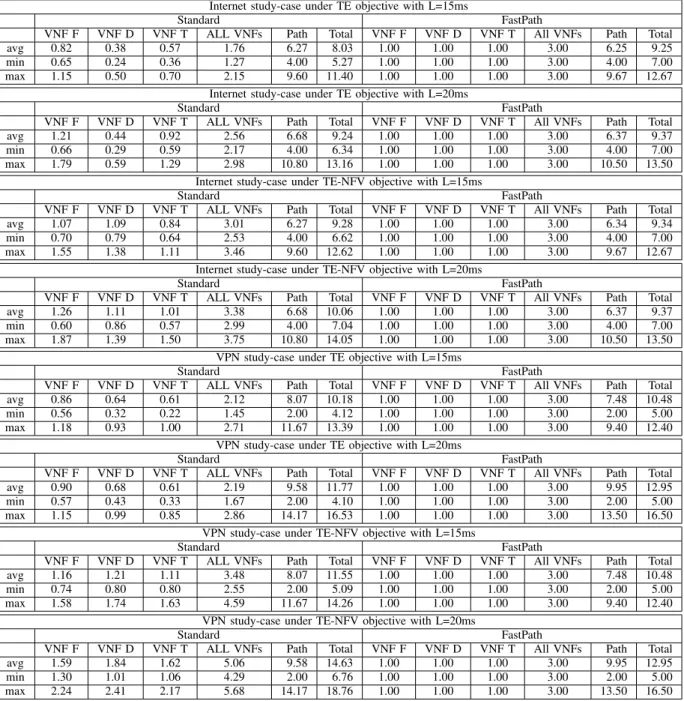
Table VIII presents the averaged, minimum and maximum results of the complete TE objective stage (using a time limit of 800s) for Internet and VPN case-studies considering the 10 random instances. We observe that for both Internet and VPN cases, the results of the complete TE objective stage of all the 10 test instances are stable: around 0.45 in Internet case and 0.60 in VPN case. The obtained results have an average optimality gap of 15%. In some instances the optimality of the solution is certified (i.e., optimality gap is 0%) and in the worst case the optimality gap is 25%. These optimality gaps may appear large, but we need to observe that the optimality gap is only an upper bound to the distance from the optimal value, and in some cases, even if the current solution shows
large gap, it can be the optimal one6. Therefore, to further
investigate this aspect, we have performed some additional tests with a longer time limit (2 hours), and we could certify that the solutions found with a smaller (800s) time limit were optimal.
TABLE VIII
AVERAGED,MINIMUM AND MAXIMUM VALUES OF THETEOBJECTIVE FORINTERNET ANDVPNCASE-STUDIES.
Standard Internet VPN L = 15ms L = 20ms L = 15ms L = 20ms Average 0.45 0.45 0.61 0.59 Maximum 0.49 0.49 0.63 0.61 Minimum 0.41 0.41 0.59 0.58 Fastpath Internet VPN L = 15ms L = 20ms L = 15ms L = 20ms Average 0.44 0.45 0.60 0.59 Maximum 0.49 0.49 0.62 0.62 Minimum 0.41 0.41 0.58 0.57
As for the NFV objective stage, it is hard to reach the optimum within the time limit of 800s. Moreover, we observe that the results depend on the case-study: with the VPN case, under both standard and fastpath latency profiles, we obtain a lower optimality gap and a smaller variation of it than with the Internet case. A possible explanation is the increased number of traffic demands with the Internet case-study, which seems to significantly impact on the computational effort.
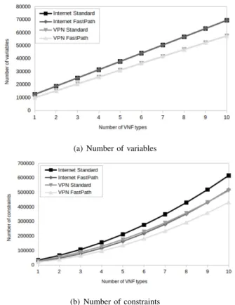
Fig. 5 illustrates the problem size with regard to the number of VNF types of both VPN and Internet case-studies. As shown
6This can be due to a poor continuous relaxation, problem quite common
TABLE IX
AVERAGED RESULTS OFNFVICOST OF THETEOBJECTIVE AND THETE-NFVOBJECTIVE UNDERINTERNET ANDVPNCASE-STUDIES,WITH THE REDUCTION RATIO OF COST FROMTETOTE-NFV (STANDARD CASE).
Standard Internet VPN
TE TE-NFV Reduction (%) TE TE-NFV Reduction (%)
L = 15ms 66.4 48.2 26.86 46.1 31 31.08
L = 20ms 59.9 52 13.05 43.2 20.9 58.66
in Table V, different model stages require different sets of variables and constraints, and the most expensive model stage in terms of number of constraints is the basic-lat-cd. In order to show how the proposed models scale with the number of VNFs, we report in Fig. 5 the dependency between the number of VNF types and the problem size (in terms of number of variables and number of constraints) of the most expensive model (basic-lat-cd model). Fig. 5 (a) shows that the number of variables increases linearly with the number of VNF types, and Fig. 5 (b) shows that the number of constraints increases nonlinearly but smoothly with the number of VNF types.
(a) Number of variables
(b) Number of constraints
Fig. 5. Dependency between the number of VNF types and the problem size. In the following, we present the analysis of the solutions behavior. We compare the two different demand case-studies (i.e. Internet and VPN) with two points of view: i) what happens when we consider the NFV cost in the objective function instead of TE (Section IV-A3 and Section IV-A4), and ii) what happens when we make stronger the bound on the end-to-end latency (Section IV-A5). Then we also compare the behavior with respect to the latency profiles (Section IV-A6).
3) TE vs. TE-NFV objective: We analyze the difference
between the results with the TE objective and the results with the composite TE-NFV objective.
• NFVI cost (Fig. 6 and Table IX): Table IX shows the
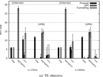
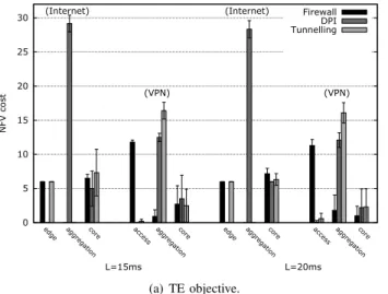
averaged total NFVI cost (i.e., the number of used CPU) obtained using the TE objective and the TE-NFV objective for both Internet and VPN cases following the standard forwarding latency profile. In the fourth (respectively seventh) column the percentage reduction in the total NFVI cost is reported. As expected, the value is reduced, but it is worth to notice that the reduction is quite significant for both Internet and VPN traffic models. Moreover, the cost reduction with VPN is more significant than with Internet, especially with a loose bound on the end-to-end latency (L = 20ms), the total cost was reduced by 58.66% in average. As we discussed in Section IV-A2, a possible explanation is the increased number of traffic demands with Internet case, which leads to possibly lower quality solutions. The variation of solutions for Internet case can also be observed in Fig. 6, where the VNF node distribution (i.e., the number of used CPU by each VNF type across NFVI edge, aggregation and core levels) is illustrated for both Internet and VPN cases with a confidence interval of 95%. In plot (b) of Fig. 6 (with TE-NFV objective), the number of VNF instances varies greatly. While in plot (a) (with TE objective), the number of VNF instances varies gently. Although there is big variation in the solutions with the TE-NFV objective, and even if the solutions are not optimal, the averaged total NFVI cost is reduced greatly with a better deployment of VNF distribution. This result shows that considering the NFV cost in the TE objective can reduce significantly the resource consumption even without reaching the optimality.
• Link utilization (Fig. 7): in addition, the link utilization
is not significantly affected by including the NFV cost minimization in the optimization goal. As illustrated in Fig. 7, in both cases with the TE goal, the aggregation links get most used. Furthermore, Internet case uses less the edge links, while VPN case uses less the core links. When taking into account the NFV cost in the objective, this behavior remains the same in both cases. This result shows that the TE-NFV goal can reduce the resource consumption without affecting the link utilization.
0 5 10 15 20 25 30
edge aggregationcore edge aggregationcore edge aggregationcore edge aggregationcore
NFV cost (Internet) (Internet) (VPN) (VPN) L=15ms L=20ms Firewall DPI Tunnelling (a) TE objective. 0 5 10 15 20 25 30
edge aggregationcore edge aggregationcore edge aggregationcore edge aggregationcore
NFV cost (Internet) (Internet) (VPN) (VPN) L=15ms L=20ms Firewall DPI Tunnelling (b) TE-NFV objective. Fig. 6. VNF node distribution across NFVI levels (standard case).
0 0.2 0.4 0.6 0.8 1 0 0.1 0.2 0.3 0.4 0.5 0.6 Cumulative probability Link utilization L=15ms (TE)
Edge links (Internet) Aggregation links (Internet) Core links (Internet)
Edge links (VPN) Aggregation links (VPN) Core links (VPN) 0 0.2 0.4 0.6 0.8 1 0 0.1 0.2 0.3 0.4 0.5 0.6 Cumulative probability Link utilization L=20ms (TE) 0 0.2 0.4 0.6 0.8 1 0 0.1 0.2 0.3 0.4 0.5 0.6 Cumulative probability Link utilization L=15ms (TE-NFV) 0 0.2 0.4 0.6 0.8 1 0 0.1 0.2 0.3 0.4 0.5 0.6 Cumulative probability Link utilization L=20ms (TE-NFV)
Fig. 7. Link utilization empirical CDFs (standard case).
• VNF forwarding latency (Fig. 8): with both Internet and
VPN demands, it increases passing from the TE goal to the NFV one. This suggests that adopting the TE-NFV goal allows a higher level of VNF sharing for both latency bound situations.
0 0.2 0.4 0.6 0.8 1 0 5 10 15 20 Cumulative probability Latency L=15ms (TE) Firewall (Internet) DPI (Internet) Tunnelling (Internet) Total (Internet) Firewall (VPN) DPI (VPN) Tunnelling (VPN) Total (VPN) 0 0.2 0.4 0.6 0.8 1 0 5 10 15 20 Cumulative probability Latency L=20ms (TE) 0 0.2 0.4 0.6 0.8 1 0 5 10 15 20 Cumulative probability Latency L=15ms (TE-NFV) 0 0.2 0.4 0.6 0.8 1 0 5 10 15 20 Cumulative probability Latency L=20ms (TE-NFV)
Fig. 8. Empirical CDFs of latency components (standard case).
TABLE X
NFVCOST FOR DIFFERENTTEGOAL RELAXATION LEVELS,WITH
TE-NFVOPTIMIZATION. Instance α = 0 α = 0.2 α = 0.4 L=15ms Standard Internet 48.2 25.8 24.9 Fastpath Internet 37.125 31 31 Standard VPN 31 28.8 28.6 Fastpath VPN 39.1 37.7 37.7 L=20ms Standard Internet 52 23.7 23.1 Fastpath Internet 38.7 34.8 31.2 Standard VPN 20.9 20.4 20 Fastpath VPN 34.9 34.8 33.8
4) Relaxing the TE constraint - sensitivity to maximum
link utilization: We perform a sensitivity analysis to put in
evidence the effect of relaxing the TE objective with respect to the NFV optimal cost, with the goal to further put in evidence the trade-off between the two objectives. With the TE-NFV objective, even if the VNF allocation cost is minimized, a minimum maximum link utilization is guaranteed. What we want to analyze is the impact of the TE bound on the NFV cost objective optimization. To this aim, starting from the TE optimal value, we perform a series of optimization steps of the NFV cost objective function, allowing this bound to be relaxed, increasingly.
Table X shows the NFV cost (average of 10 executions) under different limit of maximal link utilization (U ). We
calculate the NFV cost under U = U?+ α, with α varying
from 0 to 0.4. For both Internet and VPN cases, when α = 0,
the TE bound (U ) used for the TE-NFV phase is the U?
found in TE phase; when α = 0.4, the U used for the TE-NFV phase is around 1 (i.e., link saturation reached). The results show that a loose TE bound (link utilization) allows a better TE-NFV solution. For most cases, there is almost no reduction (or no reduction at all) from α = 0.2 to α = 0.4, which suggests that there exists a ceiling between the TE objective and TE-NFV objective: we can get better utilization of NFV resources (i.e., TE-NFV objective) by allowing relaxed
TABLE XI
AVERAGED RESULTS OFNFVICOST OF THETEOBJECTIVE AND THETE-NFVOBJECTIVE UNDERINTERNET ANDVPNCASE-STUDIES,WITH THE REDUCTION RATIO OF COST FROMTETOTE-NFV (FASTPATH CASE).
Fastpath Internet VPN
TE TE-NFV Reduction (%) TE TE-NFV Reduction (%)
L = 15ms 60.0 39.8 33.56 50.5 40 18.97
L = 20ms 59.9 38.7 37.83 47.5 35.9 21.50
link utilization limit (i.e., TE objective), however this is not always true when we reach the ceiling (e.g., other limits like VM capacity also impact NFV cost). While for case FastPath Internet L = 20ms, there is a reduction of NFVI cost with α increasing from 0.2 to 0.4. We can observe that for the same case-study with L = 15 the best objective found is 31 (both for α = 0.2 and 0.4), therefore we can attribute this change in behaviour to the not optimality of the solution in the case L = 20, rather than to a different behaviour of the system (we remind the reader that the problem is computationally very challenging, and we imposed a short time limit).
5) Sensitivity to the latency bound: We analyze the impact
of the VNF chain latency bound (L) on the results.
• NFVI cost (Fig. 6 and Table IX): as shown in Table IX,
the averaged total cost is reduced with VPN demands under both optimization goals with a loose latency bound, especially with the TE-NFV goal. This happens because, with a loose latency bound, the traffic can pass by the links with high latency (e.g., core links) to share more VNFs. On the contrary, there is a small cost increase with Internet demands under TE-NFV goal. Analyzing in a more detailed way the results, we observe that for the Internet case-study, the solver (CPLEX) has more difficulties to reduce the gap. We can deduce that making the latency bound weaker makes the location problem component (locating VNF and the NFV goal) predominant with respect to the routing one, in fact, if the latency bound is large enough the routing problem is not constrained anymore, and more routing solutions are available; this allows more freedom in the location part, and probably increases its combinatorial structure, and therefore it makes the solution of the problem com-putationally more challenging. This is also confirmed by a noticeable variability in the results, with a smaller averaged cost reduction as shown in Table IX passing from strict latency (with a cost reduction of 26.86%) to loose latency bounds (with a cost reduction of 13.05%). Moreover, we can see that with VPN demands, there is a higher dependency to the latency bound than with Internet demands; this happens because in general it is farther to send traffic demands from edge node to edge node than from edge (core) node to core (edge) node, i.e., the end-to-end forwarding path of VPN demands is in general longer than that of Internet demands, which leads to a higher dependency to the latency bound.
• Link utilization (Fig. 7): in support of the
above-mentioned analysis, we can remark that under the loose latency bound, the core links get more utilized with VPN demands. While with Internet demands, the link
utilization remains almost the same. This indicates that VPN case is more sensible to the latency bound.
• VNF forwarding latency (Fig. 8 and Table XII): the same
observation can be obtained by looking at end-to-end latency components, as shown in Table XII, the averaged total latency of VPN is always greater than Internet. Moreover, as shown in Fig. 8, the latency of each VNF and the total latency become longer with VPN demands with loose latency bound.
These observations confirm the importance of the bound for VNF chaining and placement decisions.
6) Standard vs. fastpath VNF switching: We now compare
the results with the standard VNF forwarding latency profile to those with the fastpath profile.
• NFVI cost (Fig. 6 vs. Fig. 9, and Table IX vs. Table XI):
under the TE-NFV goal, the fastpath VNF forwarding is more expensive than the standard forwarding with VPN demands, especially with a loose bound on the end-to-end latency (L = 20ms), the averaged total NFVI cost is 35.9 under the fastpath profile and 20.9 under the standard profile. While it is the opposite with Internet demands, for example, with the loose latency bound of 20ms, the averaged total NFVI cost of the TE-NFV goal is 52 under the standard profile, while it reduces to 38.7 under the fastpath profile. This happens because of the maximum traffic bound that is set under the fastpath case and that is not set for the standard case (which however brings to a higher end-to-end latency as confirmed in the last item hereafter), therefore, more VNF instances need to be deployed, which in turn increase the total cost.
• Link utilization (Fig. 7 vs. Fig. 10) : the only difference
between the link utilization under the standard and the fastpath profiles is remarkable for the case of VPN: the core links get less used with the strict latency bound of 15ms under the standard profile, while they are not used at all under the fastpath profile with the strict latency bound. However, there is no clear difference for both forwarding profiles when taking into account the NFV cost in the objective. Moreover, the behavior of the models is similar under the two forwarding profiles, when passing from strict latency limit to the loose one: under both the standard and the fastpath profiles, the core links get more utilized with VPN demands, while with Internet demands, the link utilization remains stable.