Achieving Real-time Mode Estimation through
Offline Compilation
by
John M. Van Eepoel B.S. Aerospace Engineering University of Maryland, 2000
SUBMITTED TO THE
DEPARTMENT OF AERONAUTICAL AND ASTRONAUTICAL ENGINEERING
IN PARTIAL FULFILLMENT
OF THE REQUIREMENTS FOR THE DEGREE OF
MASTER OF SCIENCE
IN
AERONAUTICAL AND ASTRONAUTICAL ENGINEERING AT THE
MASSACHUSETTS INSTITUTE OF TECHNOLOGY
FEBRUARY 2002
@ 2002 Massachusetts Institute of Technology. All Rights Reserved.
MASSACHUSETTS INSTITUTE OF TECHNOLOGY
SEP
1 0 2003
LIBRARIES
Signature of Author:
epartment of Aeronautics and Astronautics September 16, 2002
Certified by:
Brian C. Williams Professor of Aeronautics and Astronautics Thesis Supervisor
Accepted by:
Edward M. Greitzer Professor of Aeronautics and Astronautics Chair, Committee on Graduate Students
AERO
4
This page intentionally left blank.
Achieving Real-time Mode Estimation through Offline Compilation
by
John M. Van Eepoel
Submitted to the Department of Aeronautics and Astronautics on September 19, 2002 in Partial Fulfillment of the Requirements for the Degree of Master of Science in
Aeronautics and Astronautics
ABSTRACT
As exploration of our solar system and outerspace move into the future, spacecraft are being developed to venture on increasingly challenging missions with bold objectives. The spacecraft tasked with completing these missions are becoming progressively more complex. This increases the potential for mission failure due to hardware malfunctions and unexpected spacecraft behavior. A solution to this problem lies in the development of an advanced fault management system. Fault management enables spacecraft to respond to failures and take repair actions so that it may continue its mission.
The two main approaches developed for spacecraft fault management have been rule-based and model-based systems. Rules map sensor information to system behaviors, thus achieving fast response times, and making the actions of the fault management system explicit. These rules are developed by having a human reason through the interactions between spacecraft components. This process is limited by the number of interactions a human can reason about correctly. In the model-based approach, the human provides component models, and the fault management system reasons automatically about system wide interactions and complex fault combinations. This approach improves correctness, and makes explicit the underlying system models, whereas these are implicit in the rule-based approach.
We propose a fault detection engine, Compiled Mode Estimation (CME) that unifies the strengths of the rule-based and model-based approaches. CME uses a compiled model to determine spacecraft behavior more accurately. Reasoning related to fault detection is compiled in an off-line process into a set of concurrent, localized diagnostic rules. These are then combined on-line along with sensor information to reconstruct the diagnosis of the system. These rules enable a human to inspect the diagnostic consequences of CME. Additionally, CME is capable of reasoning through component interactions automatically and still provide fast and correct responses. The implementation of this engine has been tested against the NEAR spacecraft advanced rule-based system, resulting in detection of failures beyond that of the rules. This evolution in fault detection will enable future missions to explore the furthest reaches of the
solar system without the burden of human intervention to repair failed components. Thesis Supervisor: Brian C. Williams
Title: Associate Professor of Aeronautics and Astronautics
Achieving Real-time Mode Estimation through Offline Compilation
This page intentionally left blank.
Acknowledgements
I want to say thanks to my family for their love and support through my years at the University
of Maryland and the toughest two years here at MIT. The support you gave me through all of those years will come back ten-fold.
I want to especially thank Peggy Kontopanos for all of her love and support. Thank you for
carrying me through such a trying time and always being there to listen. Without her support, much of this would not have been possible.
I would like to thank most importantly my advisor, Prof. Brian Williams for all of his guidance,
discussion and ideas that have made this thesis possible. His tutelage has helped me develop as a researcher and the lessons I have learned are invaluable. I would also like to thank the
benefactors that made this research possible. Under the DARPA grant [F33615-00-C-1702], also known as the MoBies program, research into advanced diagnostic systems has been possible. Additionally, I would like to thank the Model-based Embedded and Robotics Systems (MERS) group at MIT. Their friendship, technical advice and laughter helped make understanding such difficult concepts fun. I extend many thanks to Rob Ragno, Seung Chung and Mitch Ingham who were always willing to discuss the technical issues. I also want to thank other members of the MERS group, Paul Elliott, Aisha Walcott, Andreas Wehowsky, Samidh Chakrabarti, Michael Hofbaur, Melvin Henry and Jon Kennel.
Achieving Real-time Mode Estimation through Offline Compilation
This page intentionally left blank.
Table of Contents
ABSTRACT ACKNOWLEDGEMENTS LIST OF FIGURES 1 INTRODUCTION 1.1 1.2 1.3 1.4 1.4.1 1. . 1. 1. 1.4.3 1.5 1.5.2 1.6 MOTIVATIONMODE ESTIMATION EVOLUTION
MODEL-BASED SPACECRAFT AUTONOMY MODE ESTIMATION
Inputs and Outputs
Mode Estimation Example
4.2.1 The Mode Estimation Process at 4.2.1 NEAR Spacecraft Power System
4.2.2 Mode Estimation Example
Issues in Mode Estimation Tracking System Trajectories
COMPILATION
The Basics
Compilation Example
COMPILATION AND MODE ESTIMATION_
2 CONFLICT-BASED MODE ESTIMATION.
2.1 2.2 2.2.1 2.2.2 2. 2. 2.2.3 2.3 2.3.1 2.3.2 2.3.3
MODEL-BASED MODE ESTIMATION FRAMEWORK GENERAL DIAGNOSTIC ENGINE (GDE)
GDE Inputs and Outputs Diagnosis with GDE
2.2.1 Conflict Recognition 2.2.2 Candidate Generation
Analysis of GDE
SHERLOCK
Sherlock Inputs and Outputs Diagnosis with Sherlock Analysis of Sherlock
3 COMPILATION OF CONFLICT-BASED MODE ESTIMATION 53
3.1 3.2 3.2.1 3.3 3.3.1 3.3.2 3.3.3 3.3.4 3.3.5j
MOTIVATION FOR MODE COMPILATION
MINI-ME
Mini-ME Example
MODE COMPILATION
Inputs and Outputs
Mode Compilation Algorithm Optimal Constraint Satisfaction
Dissent Generation as Optimal Constraint Satisfaction. Mode Compilation Example
Achieving Real-time Mode Estimation through Offline Compilation
53 54 55 57 57 58 60 61 63 .3 -5 11 15 15 17 18 20 21 22 22 23 27 31 31 32 33 34 36 37 37 39 40 41 43 44 45 46 46 48 51 7
3.3.6 Analysis of Mode Compilation and Mini-ME
4 CONFLICT BASED MODE ESTIMATION WITH TRANSITIONS 67
4.1 MODE ESTIMATION AND THE NEED FOR TRANSITIONS 67
4.2 SYSTEM MODEL FRAMEWORK 68
4.2.1 Hidden Markov Models 69
4.2.2 Concurrent Constraint Automata 71
4.2.2.1 Constraint Automata 72
4.2.2.2 Constraint Automaton Example 74
4.2.2.3 Concurrent Constraint Automata 76
4.2.2.4 CCA's and Mode Estimation 78
4.2.2.4.1 ME-CCA Example 81
4.2.2.4.2 Formal ME-CCA Algorithm 83
4.3 LIVINGSTONE 84
4.3.1 Livingstone Inputs and Outputs 85
4.3.2 Mode Estimation in Livingstone 87
4.3.2.1 Mode Estimation Example 90
4.3.2.2 Livingstone Diagnosis and ME-CCA 91
4.3.3 Analysis of Livingstone 92
5 COMPILED MODE ESTIMATION ERROR! BOOKMARK NOT DEFINED.
5.1 5.2 5.3 5.4 5.5 5.6 5.6.1 5.6.2 5. 5. 5.6.3
MOTIVATION FOR COMPILATION
ARCHITECTURE DISSENTS
COMPILED TRANSITIONS
ONLINE MODE ESTIMATION AT A GLANCE COMPILATION
Compiled Concurrent Automata
Transition Compilation
5.2.1 Inputs and Outputs
5.2.2 Transition Compilation Algorithm Transition Compilation Example
6 ONLINE MODE ESTIMATION _
6.1 ARCHITECTURE
6.2 INPUTS / OUTPUTS
6.3 COMPILED CONFLICT RECOGNITION
6.3.1 Dissent and Transition Trigger Basics 6.3.2 Constituent Diagnosis Generator 6.4 DYNAMIC MODE ESTIMATE GENERATION
6.4.1 Architecture
6.4.2 Dynamic Mode Estimate Generation at a Glance 6.4.3 Generate Algorithm
6.4.3.1 Generate Overview
6.4.3.2 Generate Algorithm Example 6.4.3.3 Generate Algorithm 6.4.4 Conflict-Directed A * 95 96 97 98 100 105 106 107 107 108 111 115 115 116 118 119 123 126 127 128 130 131 134 140 141
Achieving Real-time Mode Estimation through Offline Compilation
66
6.4.4.1 CDA* Heuristics 142
6.4.4.2 Conflict Direction and Systematicity 144
6.4.4.3 CDA* Algorithm 147
6.4.4.4 CDA* Example 149
6.4.5 Rank Algorithm 152
6.4.5.1 Rank Algorithm Description 153
6.4.5.2 Rank Algorithm Example 157
6.4.5.3 Rank Algorithm and Belief Update 158
6.5 MAPPING COMPILED MODE ESTIMATION TO ME-CCA 159
7 COMPILED MODE ESTIMATION ALGORITHMS 163
7.1 COMPILED CONFLICT RECOGNITION 163
7.1.1 Constituent Diagnosis Generator 164
7.2 DYNAMIC MODE ESTIMATE GENERATION 166
7.2.1 Generate 167
7.2.2 Conflict Directed A* 170
7.2.3 Rank 179
7.3 ONLINE MODE ESTIMATION 181
8 EXPERIMENTAL VALIDATION 185
8.1 NEAR SPACECRAFT POWER SYSTEM 186
8.1.1 System Block Diagram 187
8.1.2 Component Models 188
8.1.3 Charger 190
8.1.4 Battery 192
8.2 COMPILED MODEL 194
8.3 SCENARIOS AND RESULTS 196
8.3.1 Nominal Operation 199
8.3.1.1 Digital Shunt Test 199
8.3.1.2 Nominal Battery and Charger Operation 201
8.3.2 Primary Analog Shunt Failure 202
8.3.3 Failed Charger 204
8.3.4 Digital Shunt Failure 206
8.3.5 Failed Charger and Failed Analog Shunt 210
8.4 DISCUSSION 212
9 CONCLUSIONS 215
9.1 RESULTS 215
9.2 COMPILED MODE ESTIMATION 216
10 FUTURE WORK 219
10.1 COMPILED CONFLICT RECOGNITION 219
10.2 DYNAMIC MODE ESTIMATE GENERATION 220
REFERENCES 225
APPENDIX A. NEAR POWER SYSTEM MODELS 227
A. 1 NEAR POWER GENERATION ___227
A.1.1 Solar Arrays 227
A.1.2 Digital Shunts 228
A.1.3 Analog Shunts 231
A.2 NEAR POWER STORAGE 232
A.2.1 Switch 232
A.2.2 Charger 234
A.2.3 Battery 235
APPENDIX B. NEAR POWER STORAGE DISSENTS & TRANSITIONS 237
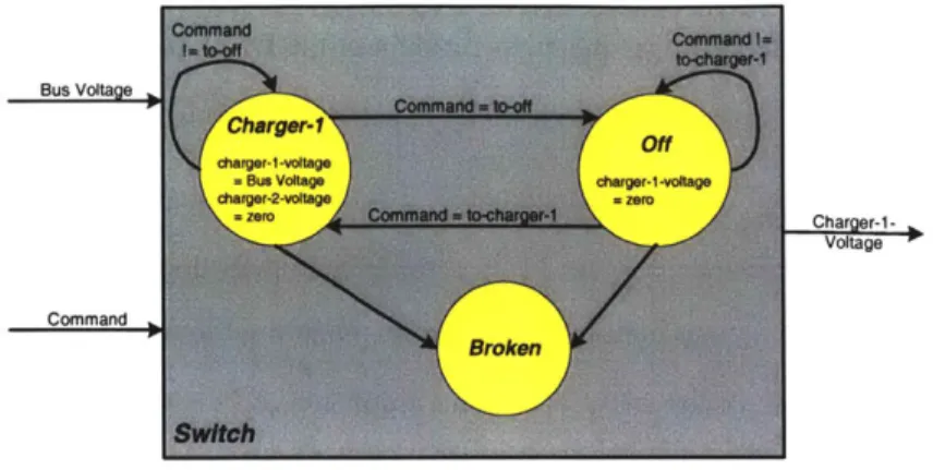
B.1 DISSENTS 237 B.2 TRANSITIONS 238 B.2.1 Charger Switch 238 B.2.2 Charger-i 239 B.2.3 Charger-2 241 B.2.4 Battery 243
APPENDIX C. ONLINE-ME DETAILED EXAMPLE 247
C. 1 OBSERVATIONS AND INITIAL MODE ESTIMATE 247
C.2 DISSENTS AND TRANSITIONS 247
C.2.1 Enabled Dissents 247
C.2.2 Enabled Transitions 248
C.3 CONSTITUENT DIAGNOSES 250
C.4 REACHABLE CURRENT MODES 251
C.5 DYNAMIC MODE ESTIMATE GENERATION 252
APPENDIX D. CME SUPPORTING ALGORITHMS 257
D. 1 DISSENT AND TRANSITION TRIGGERS 257
D.1.1 Triggering Supporting Algorithms 260
D.2 DYNAMIC MODE ESTIMATE GENERATION 262
D.2.1 Generate 262
APPENDIX E. RESULTS AND ADDITIONAL EXPERIMENTS 265
E. 1 DIGITAL SHUNT NOMINAL OPERATION 265
E.2 ANALOG SHUNT NOMINAL OPERATION 266
E.3 NOMINAL BATTERY OPERATION 268
E.4 FAILED ANALOG SHUNT 269
E.5 SOLAR ARRAY DEGRADATION 269
E.6 FAILED CHARGER 272
E.7 FAILED DIGITAL SHUNTS 273
E.8 FAILED CHARGER AND FAILED ANALOG SHUNTS 275
List of Figures
FIGURE 1-1 - MODEL-BASED EXECUTIVE ARCHITECTURE 19
FIGURE 1-2 - INPUTS AND OUTPUTS OF MODE ESTIMATION 21
FIGURE 1-3 - NEAR POWER SYSTEM 24
FIGURE 1-4 - COMPONENT MODE BREAKDOWN OF THE NEAR POWER STORAGE SYSTEM 26
FIGURE 1-5 - STEP 1 OF THE MODE ESTIMATION PROCESS 27
FIGURE 1-6 - SEARCH TREE EXPANSION USING COMPONENT MODES 28 FIGURE 1-7 - SEARCH TREE EXPANSION WITH Two COMPONENTS SHOWN 29
FIGURE 1-8 - TRACKING MODE ESTIMATES OVER TIME 32
FIGURE 2-1 - GENERAL DIAGNOSTIC ENGINE ARCHITECTURE 40
FIGURE 2-2 - SIMPLIFIED NEAR POWER STORAGE SYSTEM FOR GDE EXAMPLE 42
FIGURE 2-3 - SHERLOCK DIAGNOSTIC ENGINE ARCHITECTURE 47
FIGURE 2-4 - NEAR POWER STORAGE SYSTEM MODIFIED TO HAVE BEHAVIORAL MODES 49
FIGURE 3-1 - ARCHITECTURE OF THE MINI-ME ENGINE 54
FIGURE 3-2 -NEAR POWER STORAGE SYSTEM EXAMPLE 55
FIGURE 3-3 -MODE COMPILATION INPUTS AND OUTPUTS 58
FIGURE 3-4 -DEFINITION OF AN OPSAT PROBLEM 60
FIGURE 3-5 -ENUMERATION ALGORITHM AS OPSAT 62
FIGURE 3-6 - SWITCH AND REDUNDANT CHARGERS IN THE NEAR POWER STORAGE SYSTEM__ 63
FIGURE 3-7 -EXAMPLE SEARCH TREE FOR MODE COMPILATION 64
FIGURE 3-8 - NEXT EXPANSION OF THE SEARCH TREE FOR MODE COMPILATION 65
FIGURE 4-1 -DEFINITIONS OF A HIDDEN MARKOV MODEL 69
FIGURE 4-2 -TRELLIS DIAGRAM 71
FIGURE 4-3 - REPRESENTATION OF A CONSTRAINT AUTOMATON TRANSITION 73
FIGURE 4-4 - PROPOSITIONAL LOGIC FORM OF A CONSTRAINT 74
FIGURE 4-5 - AUTOMATON OF THE NEAR POWER SYSTEM CHARGER 74
FIGURE 4-6 - SWITCH AND BATTERY CHARGER FROM THE NEAR POWER SUBSYSTEM 77
FIGURE 4-7 - CONSTRAINT AUTOMATON FOR A SWITCH 78
FIGURE 4-8 -MODE ESTIMATION ALGORITHM FOR CCA (ME-CCA) [WILLIAMS 2, 2002] 84
FIGURE 4-9 - ARCHITECTURE OF THE LIVINGSTONE MODE ESTIMATION ENGINE 86 FIGURE 4-10 - MODE ESTIMATE CALCULATION IN LIVINGSTONE 87
FIGURE 4-11 -EXPANSION OF CONFLICTS IN LIVINGSTONE 91
FIGURE 5-1 - COMPILED MODE ESTIMATION ARCHITECTURE 97
FIGURE 5-2 - GENERAL COMPONENT, COMPILED TRANSITION 99
FIGURE 5-3 -DEFINITION OF A COMPILED TRANSITION 100
FIGURE 5-4 -DISSENTS AND COMPILED TRANSITIONS FOR NEAR POWER STORAGE EXAMPLE 101
FIGURE 5-5 -THE SET OF REACHABLE COMPONENT MODES 102
FIGURE 5-6 -EXPANSION OF FIRST SET OF CONSTITUENT DIAGNOSES 103
FIGURE 5-7 -EXPANSION OF THE NEXT SET OF CONSTITUENT DIAGNOSES 104
FIGURE 5-8 - STEPS OF MODEL COMPILATION 105
FIGURE 5-9 -INPUTS AND OUTPUTS OF TRANSITION COMPILATION 107
FIGURE 5-10 - DEPICTION OF A COMPILED TRANSITION 108
FIGURE 5-11 - TRANSITION COMPILATION AS OPSAT 109
FIGURE 5-12 - DIAGRAM OF THE CHARGER AND BATTERY OF NEAR 111
FIGURE 6-1 -INPUTS/OUTPUTS OF ONLINE MODE ESTIMATION 116
Achieving Real-time Mode Estimation through Offline Compilation
FIGURE 6-2 -INPUT/OUTPUT DEFINITIONS FOR ONLINE COMPILED MODE ESTIMATION__ 117 FIGURE 6-3 -PROCESSES WITHIN THE COMPILED CONFLICT RECOGNITION_ 118
FIGURE 6-4 -SAMPLING OF DISSENTS OF THE NEAR POWER STORAGE SYSTEM 120
FIGURE 6-5 -TRIGGERED DISSENTS FROM OBSERVATIONS 120
FIGURE 6-6 - CALCULATION OF THE REACHABLE CURRENT MODES 124
FIGURE 6-7 -DYNAMIC MODE ESTIMATE GENERATION ARCHITECTURE 127
FIGURE 6-8 - DEPICTION OF GENERATE AND CDA* RESULT 128
FIGURE 6-9 - CALCULATION OF THE RANK ALGORITHM 129
FIGURE 6-10 - SEARCH TREE OF PREVIOUS MODE ESTIMATES 131
FIGURE 6-11 - EXAMPLE OF STATE TRANSITIONS FOR THE GENERATE ALGORITHM 135
FIGURE 6-12 - INITIAL ORDERING OF THE SEARCH TREE IN THE GENERATE ALGORITHM 135 FIGURE 6-13 - SEARCH TREE AFTER IST ITERATION OF THE GENERATE ALGORITHM 136
FIGURE 6-14 - SEARCH TREE AFTER 2ND ITERATION OF THE GENERATE ALGORITHM 136
FIGURE 6-15 - SEARCH TREE AFTER 3RD ITERATION OF THE GENERATE ALGORITHM 137 FIGURE 6-16 -SEARCH TREE AFTER 4T ITERATION OF THE GENERATE ALGORITHM 137 FIGURE 6-17 -SEARCH TREE AFTER 5TH ITERATION OF THE GENERATE ALGORITHM 138 FIGURE 6-18 -SEARCH TREE AFTER 6T ITERATION OF THE GENERATE ALGORITHM 138 FIGURE 6-19 - SEARCH TREE AFTER 7TH ITERATION OF THE GENERATE ALGORITHM 139
FIGURE 6-20 -SEARCH TREE AFTER 8TH ITERATION OF THE GENERATE ALGORITHM 139
FIGURE 6-21 - EXAMPLE COST CALCULATION FOR A NODE 144
FIGURE 6-22 - DISSENT EXPANSION FROM NEAR POWER STORAGE SYSTEM (APPENDIX C) - 144
FIGURE 6-23 - CDA* EXPANSION OF CONSTITUENT DIAGNOSIS #1 149
FIGURE 6-24 - EXPANSION OF CONSTITUENT DIAGNOSIS #7 FOR CDA* 150
FIGURE 6-25 - CDA* EXPANSION OF CONFLICT #9 151
FIGURE 6-26 - EXPANSION OF CONSTITUENT DIAGNOSIS #14 152
FIGURE 6-27 - INPUTS AND OUTPUTS OF THE RANK ALGORITHM 153
FIGURE 6-28 - RANK ALGORITHM PROBABILITY CALCULATION FOR A MODE ESTIMATE 154 FIGURE 6-29 - DETERMINATION OF COMPONENT MODE ASSIGNMENT TRANSITIONS 155
FIGURE 7-1 -INPUTS AND OUTPUTS OF CONFLICT GENERATOR 164
FIGURE 7-2 -A REACHABLE CURRENT ASSIGNMENT WITH MULTIPLE PREVIOUS SOURCES ___ 164
FIGURE 7-3 - CONSTITUENT DIAGNOSIS GENERATOR ALGORITHM 166
FIGURE 7-4 -INPUTS AND OUTPUTS OF THE GENERATE ALGORITHM 167
FIGURE 7-5 -GENERATE ALGORITHM FOR DYNAMIC MODE ESTIMATE GENERATION 169
FIGURE 7-6 -INPUTS AND OUTPUTS OF THE DDA* ALGORITHM 171
FIGURE 7-7 - CONFLICT DIRECTED A* ALGORITHM 172
FIGURE 7-8 - EXPAND AND INSERT ALGORITHM SUPPORTING THE CDA* ALGORITHM 174
FIGURE 7-9 -ADD CONSTITUENT DIAGNOSIS AND ADD VARIABLE ALGORITHMS 175
FIGURE 7-10 - UPDATE ALLOWABLE ASSIGNMENTS SUPPORTING DDA* ALGORITHM 177
FIGURE 7-11 - INSERT NODE ALGORITHM SUPPORTING THE DDA* ALGORITHM 178
FIGURE 7-12 - INPUTS AND OUTPUTS OF THE RANK ALGORITHM 179
FIGURE 7-13 - RANK ALGORITHM 180
FIGURE 7-14 -INPUTS AND OUTPUTS FOR ONLINE MODE ESTIMATION 181
FIGURE 7-15 -ONLINE MODE ESTIMATION ALGORITHM 182
FIGURE 8-1 - ARTIST'S DEPICTION OF THE NEAR SPACECRAFT 185
FIGURE 8-2 -NEAR POWER SYSTEM SCHEMATIC 187
FIGURE 8-3 -SCHEMATIC OF SIMPLIFIED NEAR POWER SYSTEM 188
FIGURE 8-4 - NEAR POWER SYSTEM BLOCK DIAGRAM 189
FIGURE 8-5 - CONSTRAINT AUTOMATON OF THE NEAR POWER SYSTEM CHARGERS 190
FIGURE 8-6 - CONSTRAINT AUTOMATON OF THE NEAR POWER SYSTEM BATTERY 192
FIGURE 8-7 -COMPILED TRANSITION FUNCTION FOR EACH COMPONENT 195
FIGURE 8-8 - RULES FOR THE NEAR POWER SYSTEM 197
FIGURE 8-9 - CME OUTPUT FOR DIGITAL SHUNT NORMAL OPERATION 200
FIGURE 8-10 -CME ENGINE OUTPUT FOR NOMINAL CHARGER AND BATTERY OPERATION 202
FIGURE 8-11 - CME OUTPUT FOR A FAILED ANALOG SHUNT 204
FIGURE 8-12 - CME OUTPUT FOR FAILED CHARGER 206
FIGURE 8-13 - CME DIAGNOSIS OF THE DIGITAL SHUNT FAILURE 207
FIGURE 8-14 - CME OUTPUT FOR A FAILED DIGITAL SHUNT 210
FIGURE 8-15 -CME RESULTS ON DOUBLE FAILURE WITH THE ANALOG SHUN AND CHARGER_ 211
FIGURE 10-1 -EXAMPLE TRANSITION SYSTEM FOR NEW HEURISTIC 221
FIGURE A-I - CONSTRAINT AUTOMATON FOR THE NEAR POWER SYSTEM SOLAR ARRAYS __ 227
FIGURE A-2 - CONSTRAINT AUTOMATON FOR THE NEAR POWER SYSTEM DIGITAL SHUNTS _ 229
FIGURE A-3 - CONSTRAINT AUTOMATON FOR THE NEAR POWER SYSTEM ANALOG SHUNTS _ 231 FIGURE A-4 - CONSTRAINT AUTOMATON FOR THE NEAR POWER STORAGE SWITCH 233
FIGURE C-I -NEAR POWER STORAGE SYSTEM 247
FIGURE C-2 - SPACE OF POSSIBLE COMPONENT MODES 251
FIGURE C-3 -EXPANSION OF CONSTITUENT DIAGNOSES 1 252
FIGURE C-4 -EXPANSION OF CONSTITUENT DIAGNOSES 7 252
FIGURE C-5 -EXPANSION UNDER 'CHARGER-1 = OFF NODE OF CONSTITUENT DIAGNOSES 3 _ 253
FIGURE C-6 - EXPANSION OF CONSTITUENT DIAGNOSES 9 254
FIGURE C-7 - EXPANSION OF THE SET OF CONSTITUENT DIAGNOSES #4 254
FIGURE C-8 - EXPANSION OF CONSTITUENT DIAGNOSES 12 UNDER THE GREEN PATH 255
FIGURE D- 1 - INPUTS AND OUTPUTS OF THE DISSENT AND TRANSITION TRIGGERS 257
FIGURE D-2 - DISSENT TRIGGER ALGORITHM 258
FIGURE D-3 - TRANSITION TRIGGER ALGORITHM 259
FIGURE D-4 - UPDATE-TRUTH ALGORITHM SUPPORTING COMPILED CONFLICT RECOGNITION 261
FIGURE D-5 - COMPRESSION OF PREVIOUS BELIEF STATE 261
FIGURE D-6 - COMPRESS STATES ALGORITHM 262
FIGURE D-7 - INSERT-IN-ORDER ALGORITHM SUPPORTING THE GENERATE ALGORITHM 263
TABLE 6-1 - EXAMPLE OF TRUTH VALUES FOR ASSIGNMENTS 121
Achieving Real-time Mode Estimation through Offline Compilation
This page intentionally left blank.
1 Introduction
1.1
Motivation
Spacecraft face many challenges in current and future missions due to the harsh environment of space and the complexity of spacecraft systems. Coupled with these challenges, additional problems are created by the growing number of spacecraft being developed, system design and manufacturing flaws and the increasing complexity of missions. These can cause unpredictable spacecraft behavior as well as component and system failures, which can have deadly repercussions. Spacecraft require a technology to increase robustness in the face of these problems. Spacecraft autonomy, more specifically fault management, provides a solution that permits space exploration and spacecraft to move beyond these obstacles. Fault management embodies the spacecraft with the intelligence that allows it to reason about faulty components and work around them to continue to achieve its mission goals. Spacecraft with this capability reduce the impact of failures and increase the likelihood of mission success.
Fault management systems can be designed at varying levels and complexities. In the most basic sense, a spacecraft can be considered autonomous if it has the ability to detect pre-specified failures and take repair actions. This type of autonomous system is based on a set of scenarios developed by human modelers and embedded in the spacecraft processor. Anything outside of these scenarios causes the spacecraft to radio Earth for further instructions. In order to develop more complex scenarios, a human would have to reason about multiple components, their individual behaviors and failures. A more sophisticated fault management system automates this reasoning using a model of the spacecraft and the foundations of artificial intelligence. A system
Achieving Real-time Mode Estimation through Offline Compilation
of this type reasons through component behaviors and interactions as prescribed by the model. These two distinct approaches demonstrate the difference between current fault management in spacecraft -rule-based systems that give repair actions for only certain specified faults, and the model-based approach that determines system behavior and repair actions for many faults.
The necessity of fault management is best demonstrated by looking at the needs of past and future missions. Take as an example the Mars Polar Lander. This spacecraft was scheduled to land in the polar regions of Mars, an environment with assumedly harsh conditions. Upon descent, the spacecraft prematurely cut its engine while it was still approximately 130 ft (40 m) off of the ground. This command likely caused the spacecraft to plummet to the surface and break apart on impact. It was determined that after the landing legs had deployed, a failed sensor mistakenly read that its landing leg had touched the surface. A more sophisticated fault
management system would have enabled the spacecraft to compare the readings of all sensors, including the laser range finder. With a majority of the landing sensors reading
'no-ground-contact', and the laser range finder reading a distance of 40 m, it could have reasoned that there
was a faulty sensor and ignored it. This reasoning capability protects the spacecraft from component failures, allowing it to recover and complete its mission.
Take as another example the MESSENGER [JHUAPL, 2002] mission to Mercury currently being built and operated out of the Applied Physics Lab at Johns Hopkins University. System failures caused by the harsh environment around Mercury are a primary challenge of this mission. In addition, due to the time delay of communication, the dependence of the spacecraft on transmissions from Earth hinders science collection and the completion of mission goals. Spacecraft autonomy would enable the spacecraft to independently plan and execute activities, and perform operations to maintain the health of the spacecraft. It offers the MESSENGER spacecraft a robust approach to handling failures and completing mission goals with minimal contact with Earth.
These examples give a variety of possible applications of basic and more sophisticated levels of fault management and autonomy. These are essential for missions as they explore further into our solar system and as spacecraft grow in complexity. If something unexpected occurs, the
spacecraft could recover and still complete the activity without ever having to contact the ground for help. For the reasons detailed here, model-based autonomy and fault management will have
a prominent role in the development of future spacecraft.
1.2
Mode Estimation Evolution
A component of the fault management system is mode estimation, which determines the
behavior of the system using current sensor information. Mode estimation determines if components are faulty, but also tracks the nominal behavior of the system. This is a key aspect that enables an autonomous system to accurately control the spacecraft systems.
An accurate mode estimation engine must have several key attributes to achieve the goal of detecting failures and determining system behavior accurately. The engine must be capable of detecting single and multiple failures, using multiple sources of information to determine system behavior, and have the ability to rank diagnoses of the system. Additionally, as available resources, including time, computational power and storage space, for fault management on board a spacecraft dwindle it becomes necessary to require faster response times and smaller memory allocation for these software processes. The mode estimation engine that has been developed, Compiled Mode Estimation (CME), was designed to address these concerns and be an improvement over previous mode estimation approaches.
Mode estimation leverages models and reasoning algorithms to determine the behavior of the system. Previous mode estimation engines required many computations in order to estimate the system behavior using these models and the current sensor information. CME has been
developed to reduce the number of computations at run-time and address the real-time performance issues of these previous engines. CME is divided into two steps, an offline model compilation phase and online mode estimation engine. In the offline stage, the compiled model is generated by removing particular information that is costly to determine at run-time. This allows for the design of an any-time algorithm that can determine the system behavior in the online phase. CME addresses the concerns faced by current and future missions by providing a
Achieving Real-time Mode Estimation through Offline Compilation
capability that can identify failures and nominal system behavior, and provide these for a real-time system.
Additionally, previous mode estimation engines have the potential to increase the risk of a mission. The benefits of developing models of the system and using reasoning algorithms to determine system behavior are to have the ability to identify many behaviors of the system, not just those that can be specified by a human modeler. However, the results of previous engines were unpredictable prior to the operation of the system. One of the key benefits of CME is it makes the possible diagnoses of the system explicit before the system operates due to the compiled model. This enables a human modeler to inspect the diagnoses for correctness.
Compiled Mode Estimation only provides one capability of a larger autonomy system. The following section presents the architecture of an autonomy system to highlight the utility of mode estimation, and the capability of an autonomous system.
1.3
Model-based Spacecraft Autonomy
Several different methods have been explored to engineer an autonomous system for spacecraft. To date, the two main approaches utilized have been rule-based and model-based systems. Rule-based autonomy specifies repair actions in response to observations of undesirable sensor information. These repair actions are based on a fixed set of scenarios identified by human modelers that have reasoned through the spacecraft component interactions. Model-based autonomy produces a robust approach to handling system failures by considering a larger set of spacecraft behavior using models and reasoning algorithms. It offers a way for human modelers to convey knowledge of failures in terms of common sense engineering models of spacecraft components. These models enable reasoning algorithms to determine the current behavior of the spacecraft, identify failures, diagnose and repair using sensor information. Model-based autonomy was selected as the basis of this research as it allows the spacecraft to reason through component interactions independent of a human modeler.
A model-based autonomous system is best understood through an explanation of its main
components, and their interactions. Shown in Figure 1-1 is the paradigm of a model-based
program and a model-based executive [Williams 2, 2002]. Here the fault management portion is labeled as the 'Deductive Controller'.
RMPL Model-based Executive
Figure 1-1 -Model-based Executive Architecture
The architecture shows the model as the starting point, described in the Reactive Model-based Programming Language (RMPL) [Ingham, 2001]. The model has two different levels, a control program and a system model. The control program encodes a model of the intended behavior of the spacecraft. This is a way to describe sequences of actions that achieve certain goals, such as telling the propulsion system to thrust. The system model encodes the spacecraft component behavior and their interactions.
The model-based executive acts as a high level controller using the estimated behavior of the spacecraft to determine control actions, encoded as 'commands' in Figure 1-1, which place the spacecraft in a desired configuration. The model-based executive is comprised of three major components, the Sequencer, the Mode Reconfiguration engine, and the Mode Estimation engine. The Sequencer's task is to execute a specified sequence of actions, where the actions are specified within the control program. These actions are then translated by the Sequencer to a
'configuration goal', which specifies the desired modes for the spacecraft components. The Mode Reconfiguration engine then uses these configuration goals, the current mode estimate of
the system and the system model, to determine the control actions, or commands, to apply to the spacecraft components in order to achieve the configuration goal. The final piece of the architecture is the Mode Estimation engine that uses the observations, commands and the system model to determine the current mode estimate of the system. Observations represent the current readings of sensors in the spacecraft system and are vital to determining the current behavior of
Achieving Real-time Mode Estimation through Offline Compilation
the spacecraft. The Mode Estimation and the Mode Reconfiguration engines work together to provide the spacecraft with a fault management capability. The mode estimates represent the current behavior of the system, and are used to exact repairs on the system determined by the
Mode Reconfiguration engine.
A mode estimate represents the Mode Estimation engine's best determination of the behavior of
the components in the spacecraft. The behavior of a component is encoded in the system model, and the task of Mode Estimation is to determine the best mode for each component in the system that is consistent with the observations, commands and the model. The Mode Estimation engine can be thought of as the doctor on the spacecraft. It identifies the behavior of the spacecraft including normal or faulty operation. It diagnoses the components' behavior by determining the most likely component modes. Estimating system behavior is an essential task for an autonomy architecture to correctly and accurately control the system. Mode estimation provides an accurate representation of the current behavior of the system, which is needed to control the system. It is essential to increase the accuracy of mode estimation to enable the correct control on the spacecraft by the model-based executive.
CME seeks to increase the accuracy of mode estimation and provide an engine with the
capabilities described previously. However, to understand the process of determining system behavior, requires developing a very primitive mode estimation engine and demonstrating this using an example. The following sections present an approach to mode estimation in 1.4, followed by the enhancements to this process using model compilation in Section 1.5.
1.4
Mode Estimation
The Mode Estimation engine maps the system model, the observations and commands to a set of component modes that reflect the behavior of the system. The task of mode estimation is to choose the proper component modes that are consistent with the model constraints, and also agree with the observations and commands. Mode estimation is an example of the task of inferring hidden state [Wiliams 2, 2002]. Since the modes of these components cannot be directly obtained, hence hidden, then they can only be estimated using the system model, observations
and commands. In the case of spacecraft systems, there are only observations that give insight into the behavior of the components in the spacecraft. Mode estimation is framed using the theory of hidden state problems, the foundations of logical inference and the theory of Hidden Markov Models.
The process to estimate these component modes is best understood by first discussing the inputs and outputs of the mode estimation algorithm, and then demonstrating the process on an example spacecraft system. The example gives a context and a grounded way to discuss the basic steps of mode estimation.
1.4.1 Inputs and Outputs
The mode estimation engine uses the system model, the current observations and commands to determine an estimate of the component behavior, represented by a mode estimate. These have been discussed briefly, but a more thorough definition of each of these inputs and outputs is now given. Figure 1-2 depicts these inputs and outputs.
Moe
Obse ~ Mode Md
Estimation Estimate
Figure 1-2 -Inputs and Outputs of Mode Estimation
The 'system model' represents the behavior of each component in the system being monitored.
The components are modeled by a set of discrete modes. Each discrete mode is expressed by a set of constraints that describe the component behavior within the mode and probabilistic transitions to other modes of the component. These constraints relate the observations, commands and intermediate variables. The 'observations' represent the sensor information of the system. The 'commands' represent the control actions that the Model-based Executive may perform on the system. The intermediate variables are an internal variable in the system model that enables communication between different components.
Achieving Real-time Mode Estimation through Offline Compilation 21
The output 'mode estimate' is an assignment of modes, one for each component in the system that is consistent with the system model, the observations and the commands. There are many mode estimates of the system at any given time, which are ordered using probabilities. This assignment of component modes is only an estimate since the system model includes probabilistic transitions. Probabilistic transitions are necessary to capture the behavior of failures and intermittency within a real system.
1.4.2 Mode Estimation Example
There have been many systems that solve the mode estimation problem [deKleer, 1987, deKleer,
1989, Williams 1996, Kurien, 2000, Hamscher, 1992]. This section presents the basic steps of
mode estimation, followed by a description of a spacecraft system, and ends with a description of mode estimation applied to the example spacecraft system.
1.4.2.1
The Mode Estimation Process at a Glance
The 'system model', as described before, is comprised of models of each component in the
spacecraft system. Each of these models includes modes that characterize different behaviors of the component within the overall spacecraft system. The modes are described by specified model constraints that capture the behavior of that mode and by probabilistic transitions to modes within the same component model.
Mode estimation determines the set of component mode assignments that are consistent with the constraints associated with the component modes and the transitions. To accomplish this, mode estimation must perform two key steps:
1. Determine a set of likely next mode assignments given likely mode assignments in
the previous state and the transitions.
2. Choose the most likely, current component modes that are consistent with the mode constraints, the observations and control values.
Mode estimation computes the likely next mode assignments by choosing transitions that mention mode assignments in the previous state and storing the targets of the transitions in the set of likely next mode assignments. The second step of mode estimation computes the current mode estimate by searching for combinations of component modes and determining if they are consistent with the constraints. Effectively, the mode estimation process must choose the optimal component modes, optimal due to the probabilistic transitions. Mode estimation is then framed as an optimal constraint satisfaction problem where the solution is the set of component modes that gives the highest probability, and that also satisfy the model constraints.
The process of mode estimation gives the system the ability to determine component behavior accurately and at a higher level than the continuous dynamics of the system. Mode estimation has the ability to determine faulty components in terms of discrete modes. For instance, mode estimation is able to determine that a valve is stuck-open instead of specifying this in terms of continuous sensor readings, such as flow = 0.54 ft3/min. This high level specification of the
system behavior enables the Model-based Executive to determine recovery actions.
1.4.2.1
NEAR Spacecraft Power System
The steps of the basic mode estimation are best demonstrated by example. Our example is taken from the Near Earth Asteroid Rendezvous (NEAR) mission, operated by the Johns Hopkins University Applied Physics Lab in Columbia, MD. The mission launched in February of 1996, rendezvoused with the Eros asteroid on February 14, 2000. The spacecraft lasted much longer than anticipated and performed a groundbreaking maneuver. It landed on the surface of the Eros asteroid in February of 2001, and the spacecraft continued to transmit data back to Earth until it ran out of power in February 28, 2001.
The NEAR spacecraft has eight systems interacting together to maintain the health of the spacecraft, to control the attitude, to collect science information, to enable communication, and to provide power to the spacecraft. The power system of the NEAR spacecraft is chosen as the example system for its complexity and familiarity from everyday life. For instance, the interactions of a battery and a charger are easy to understand since they are in cars, trains, cell phones, etc. However, the power system of the NEAR spacecraft does offer interesting
Achieving Real-time Mode Estimation through Offline Compilation
complexities due to the collection of power in space. For instance, the power generated by the solar arrays must be regulated to a specific level so that the sensitive instruments are not harmed.
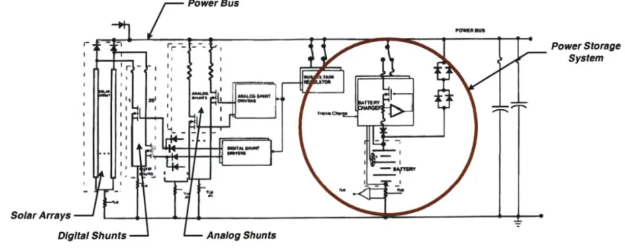
The NEAR Power sub-system is shown below in Figure 1-3. The example focuses in particular on the NEAR Power storage sub-system, highlighted with a circle in the figure.
Power Bus
Power Storage System
Solar Arrays
Digital Shunts Analog Shunts
Figure 1-3 -NEAR Power System
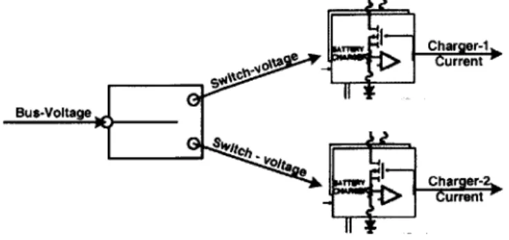
The power system is built up using solar arrays that generate power, digital and analog shunts that regulate the power, and components to store the power, built using a switch, redundant battery chargers and a battery. The NEAR Power system is an example of a direct energy transfer (DET) power system [Wertz, 1999]. All of the incoming power gathered from the solar arrays is initially put on the power bus. However, this incoming power might be too much for the power bus and spacecraft components to handle. The digital and analog shunts are placed in the system to prevent this excess power from affecting the spacecraft components. These shunts act to dissipate the excess power when they are enabled. These shunts are supported by the analog and digital shunt drivers, and bus voltage regulator that determine when shunts should be enabled or disabled.
The next stage of this power system is the power storage system. The components of the power storage system are a switch, two redundant chargers, and a NiCd battery. The available sensors for the power storage system measure the incoming bus voltage, the outgoing battery voltage, and the temperature of the battery. The switch is linked to the redundant chargers to change the charger that receives the bus voltage. This switch guarantees that only one charger can charge
the battery at any given time. The chargers use the voltage from the switch to output a current that charges the battery. The chargers have two different charging modes, a trickle charge and a full-on charge. The trickle charge is used if the battery is nearly fully charged so as to keep it at a full charge. This mode delivers a small current to the battery. The full-on charge is used if the battery charge is low. This mode delivers the maximum current possible to charge the battery as quickly as possible. The battery behavior is based on the level of charge remaining in the battery and the current rate of discharge of the battery. The indicator of the level of charge in the battery is the temperature, since there is no direct sensor for the level of charge. The indicator for the rate of discharge of the battery is the voltage sensor, depicted between the bottom of the battery and the power bus in Figure 1-3. These observations indicate if the battery is currently discharging, charging or full.
The power generation system, made up of the solar arrays, shunts and shunt drivers, and the power storage system interact to give the voltage required by the NEAR spacecraft. The power storage system reacts to the needs of the spacecraft and the available power generated from the power generation components. If the solar arrays provide too much power, as is the case when the spacecraft is near Earth, then the power storage system stores this extra power, up to the capacity of the battery. If the solar arrays cannot provide enough power for the spacecraft, then the power storage system reacts automatically and supplies the necessary voltage. The reason that the solar arrays provide too much power near Earth is that the solar arrays are designed to provide the required power for the spacecraft when it is at the asteroid, Eros. Since the asteroid is further away from the sun than Earth, the solar power available is much less. It is for these reasons that the power system has a means to dissipate, as well as store, excess power.
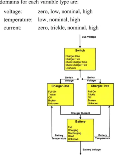
The power storage system is made the focus of further discussion and example because of its component interactions and interesting component modes. The modes of the components and interactions between the components are detailed in Figure 1-4. The different types of variables and their domains are listed below.
Observable: bus-voltage, battery-voltage, battery-temperature
Intermediate: switch-voltage, charger-current
Component: switch, charger-one, charger-two, battery
Achieving Real-time Mode Estimation through Offline Compilation
Command: NONE
The domains for each variable type are: voltage: zero, low, nominal, high temperature: low, nominal, high
current: zero, trickle, nominal, high
Bus Voltage Switch Charger-One Charger-Two Stuck-Charger-One Stuck-Charger-Two Unknown Switch Switch
vod ako Voltage
Charger-One Charger-Two
full inicaing o tecarg rthtitkl onynesTo rckecaretekateylheeh | Charge Current
Battery Full
Chrging
temperaure isnominal this eans tat te bicatryisntflidiaigtrtecageyhti
Battery Voltage
Figure 1-4 - Component Mode Breakdown of the NEAR Power Storage System
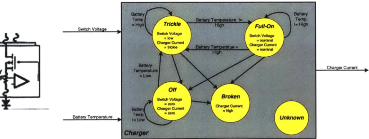
The power storage system has several design characteristics worth noting. For instance, Figure 1-4 and Figure 1-3 shows the chargers using the temperature of the battery as an input. This sensor reading indicates the level of charge in the battery, which is used by the charger to determine how to charge the battery. When the temperature is high, this means that the battery is full, indicating to the charger that it only needs to trickle-charge the battery. When the temperature is nominal, this means that the battery is not full, indicating to the charger that it should apply the maximum current possible, putting the charger in thefull-on mode.
The component modes shown here each have associated constraints describing their behavior. The switch modes, for either 'charger-1' or 'stuck-charger-1', are used to pass the incoming
bus-voltage to charger-1. The difference between the two is that the mode 'stuck-charger-1' is a
failure mode indicating that the switch cannot move from the position for charger-1. The modes of the charger model the type of charge being applied to the battery. In the full-on mode, the charger is sending a nominal current to the battery to give it the highest charge possible. In the
trickle mode the charger sends only a trickle-charge to the battery to keep the charge level full.
The broken mode for the chargers may be deduced by detecting that the output 'charger-current' is high. The model for the charger is built using the switch voltage and the output charger current to model the component modes, and using the battery temperature to model the transitions between modes. For the battery, the 'full', 'charging' and 'discharging' modes model the behavior described earlier using the input current from the charger and the output battery voltage. The full representation of these component models is given in Appendix A.
1.4.2.2
Mode Estimation Example
This section demonstrates the two basic steps of mode estimation using the NEAR Power Storage system. Recall that the first step of mode estimation assumes that there already exists a previous mode estimate. Using the transitions and the previous mode estimate, the algorithm determines the set of component modes that are reachable in one time step. To determine this, the algorithm first finds the transitions whose source are the component modes in the previous mode estimate. The constraints are then extracted from the transitions and added to the model constraints. This is represented graphically in Figure 1-5.
Previous Mode Reachable Current Estimate (St),P(S(I)) Modes (M101-11))
Switch Switch Charger-One Charger-One Stuck-Charger-One Stuck-Charger-Two Unknown Charger-One Charger-One Off Off Trickle Broken Unknown Charger-Two Oft Charger-Two Off Trickle
Battery Broken Unknown
Discharging Battery
Dcrcharging
Charging
Dead
Unknown
Figure 1-5 -Step 1 of the Mode Estimation Process
Achieving Real-time Mode Estimation through Offline Compilation
Depicted on the figure above is the previous mode estimate, which is the pair (S"t, P(SNt)). This pair denotes the state, S(t), as a choice of a single mode for each component in the system, and the probability of this mode estimate, P(S(t)). For this example, the probability of the previous mode estimate is 1. The figure denotes the set of component modes that are reachable in the current time step, 't+i', and these are determined by the transitions. For instance, in the case of the
switch, the 'charger-2' mode is not allowed in the current modes because the switch only
transitions to 'charger-2' if charger-i fails. Since charger-i was 'off in the previous mode estimate, then the transition of the switch from 'charger-i' to 'charger-2' is not allowed.
To summarize, the first step of mode estimation has determined the transitions that are allowed from the previous mode estimate, and calculated the set of reachable current component modes. The mode estimation algorithm has added the constraints from all the transitions into the model constraints and extracted the model constraints from the reachable current component modes. These constraints and this set of reachable current component modes are then used in the second step of mode estimation.
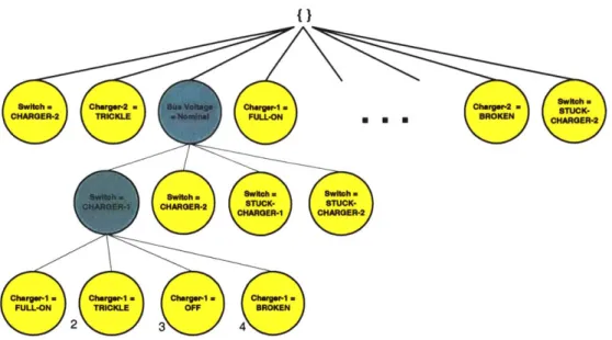
The second step of mode estimation determines which sets of reachable component modes are consistent with the model constraints and the observations. In order to determine all different combinations of the component modes, the calculation must be performed methodically. The sets of current component modes are generated through systematic search. As a straw man, mode estimation uses chronological search to determine the sets of component modes, depicted in Figure 1-6.
{}
Figure 1-6 -Search Tree Expansion Using Component Modes
This first expansion shows the search using the current component modes of the switch. The search then continues to expand the tree until it determines a mode to each component in the power storage system. The search follows the first leaf of the tree, 'switch = charger-i' and
expands the next component under it, charger-1. Figure 1-7 depicts this expansion.
{}
Switch = Switch = Switch =
Stuck- Stuck- Unknown Charger-1 Charger-2
Charger-1 Charger-1 Charger-1 Charger-1
= Trickle = OFF = Broken
Figure 1-7 -Search Tree Expansion with Two Components Shown
The search would continue until it determined a complete set of component modes. From the listing of current component modes in Figure 1-4, the first full choice of component modes is:
(switch = charger-1), (charger-i = trickle), (charger-2 = trickle), (battery = charging)
This set of reachable component modes must be checked to insure that it is consistent with the mode constraints. To demonstrate this process, consider the following current observations of the system.
(bus-voltage = nominal), (battery-temperature = nominal), (battery-voltage = nominal)
To determine if the mode estimate is consistent, mode estimation begins by propagating variable values through the model constraints of the component modes.' This process enables mode estimation to predict values for many of the observation and intermediate variables in the system. For a mode estimate to be consistent, any value it predicts must agree with the current observations. Using the mode estimate from above, the remaining values within the system that must be determined are the switch-voltage and the charger-current, one of each per charger.
'Using a complete satisfiability algorithm, if no variable value is predicted for a variable, an assignment must be found that is consistent with the observations. [Williams, 2002]
Achieving Real-time Mode Estimation through Offline Compilation
Beginning at the switch, and using the observation 'bus-voltage = nominal', this is propagated
through the component model for 'switch = charger-i', which gives 'charger-1.switch-voltage =
nominal' and 'charger-2.switch-voltage = zero'. These values are then propagated through the
models of the chargers for 'charger-i = trickle' and 'charger-2 = trickle'. The resultant value
for the output of charger-i is 'charger-1.charger-current = trickle'. When propagating through
the component model for the mode 'charger-2 = trickle', the input switch-voltage must be 'nominal' or 'low' according to the mode constraints. This results in conflicting results for the variable 'charger-2.switch-voltage'. The mode estimation algorithm then throww out this set of
component modes as an inconsistent mode estimate.
Once mode estimation determines if a set of component modes is consistent or inconsistent, it uses the search tree to generate another set of component modes to test for consistency. This process repeats until the generation of mode estimates has explored a certain amount of the probability space, or the entire search tree is explored and all consistent mode estimates have been generated. The steps of the mode estimation process described here have:
1. Generated a set of current component modes using the transitions and a previous
mode estimate.
2. Used this set of current component modes to generate mode estimates
3. Tested each for consistency, and kept those that are consistent.
The algorithm described above is an overly simplified approach to calculating these key steps. However, even this simple algorithm contains many of the key attributes of a mode estimation engine, described in section 1.2. It is able to use multiple sources of information to determine the modes of components, and it is able to determine single and multiple faults. Finally, the algorithm ranks mode estimates using probabilistic transitions. This information however can be used more efficiently in the search. There have been many algorithms designed to perform a variant of mode estimation [deKleer, 1987, deKleer, 1989, Williams, 1996, Kurien, 2000,
Ingham, 2001]. Earlier mode estimation engines [deKleer, 1987, deKleer, 1989] did not have
transitions in the models of components.
1.4.3 Issues in Mode Estimation
The mode estimation algorithm described in the previous section is a brute force approach to generating mode estimates. The algorithm generates many combinations of component modes that are inconsistent with the model constraints and observations. The problem with generating these inconsistent mode estimates is the time spent in determining that it is inconsistent. The propagation of model information and the search over possible component modes is an NP-hard problem resulting in an exponential computation in the number of components.
The test for consistency of mode estimates is costly due to the search for possible assignments in the system. The example above demonstrated this search and the ensuing propagation of variable values. Notice in the example above the amount of time taken to determine the values of the 'charger-J.switch-voltage' and the 'charger-2.switch-voltage'. In particular, in order to determine these values, mode estimation performed a search over variables whose values were not determined by propagation. This results in an overall exponential computation. As the number of components in the system increases, so do the number of variables that must be determined for each mode estimate. Determining these values is the computational bottleneck of mode estimation.
1.4.4 Tracking System Trajectories
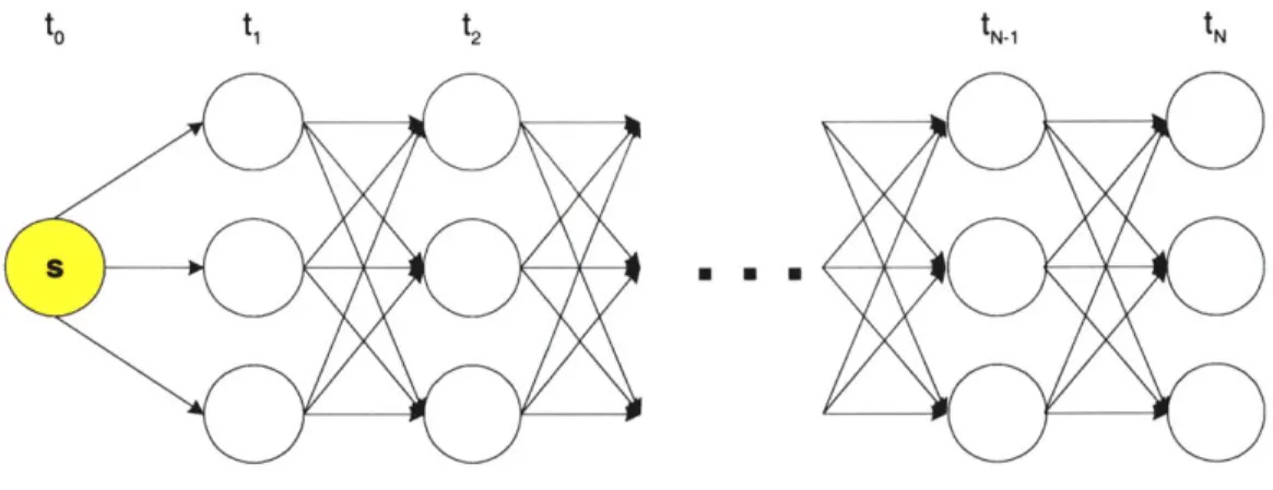
Recent mode estimation engines have incorporated transitions into the models of system components to enhance the accuracy of mode estimates [Williams, 1996, Kurien 2000]. These systems tracked the behavior of the system over time by maintaining the likely mode estimates at each time step. The trajectory tracking is depicted in Figure 1-8, where one path (noted in red) is kept at each time increment.
Achieving Real-time Mode Estimation through Offline Compilation
Figure 1-8 -Tracking Mode Estimates Over Time
Tracking mode estimates over time gives the benefit of diagnosing complex failures that evolve over time. Trajectory tracking requires determining if certain transitions between states are allowed. Determining this requires a consistency test, similar to the one described for mode constraints. Tracking likely trajectories limits the computations required to determine if taking a transition is consistent with the system model. However, only tracking likely mode estimates limits the diagnoses of the system to these likely trajectories, but a less likely trajectory could become a likely one in the future as more observations are collected to refine the mode estimates.
Systems that track likely trajectories may miss these types of diagnoses.
An alternative approach is to track consistent mode estimates from one time step to the next. This approach enables more accurate estimation of the system behavior since states, not trajectories, are tracked over time. A mode estimation engine with this capability tracks the evolution of many mode estimates, requiring many more computations than the tracking of likely trajectories. However, the benefits of tracking mode estimates over time is the increased accuracy of the mode estimates and the ability to diagnose complex failures. CMIE develops an approach for tracking mode estimates that is enabled by the compiled model.
1.5
Compilation
The performance of mode estimation may be improved by compiling the system model before the system needs the mode estimates. This process removes the need to determine consistency of mode estimates by identifying all sets of infeasible component modes in the system and compiling transitions to remove the need for consistency determination at run-time. The
compilation process is the key enabling technology for the next evolution of mode estimation for spacecraft, CMIE.
Compilation enables the mode estimation process to perform fewer computations to determine consistent mode estimates, as well as making the reasoning process of mode estimation more explicit. Compilation is a two step process of compiling the mode constraints and the transitions. The compilation of the model constraints results in generating conflicts, which are a more intuitive representation of the model constraints than an uncompiled model. The conflicts represent infeasible assignments that correspond to particular observations. These are easier to grasp and inspect by a human, making the diagnoses more explicit. By determining all conflicts in an offline process, the exponential computation of consistency is no longer performed at the time of execution.
The compilation process that has been designed is discussed first, followed by a simple example to demonstrate the compilation process. This discussion focuses on the compilation of mode constraints. The compilation of transitions is presented in Chapter 4.
1.5.2 The Basics
Recall, from the mode estimation example (Section 1.4.2.2), that the mode estimate was inconsistent with the system model and observations. To determine the inconsistency, the algorithm identified a discrepancy between the observed value for the 'charger-2.switch-voltage' and the value predicted from the system model. The identification of this discrepancy leads to a conflict. A conflict is defined as a set of component modes that cannot be true given the current observation. In the case of the example, the resulting conflict would be:
-, [ (charger-2 = trickle) ]
This states that it is inconsistent to assign charger-2 the mode trickle because of the discrepancy between the observation and the prediction. Identifying these discrepancies and determining the infeasible sets of component mode assignments, conflicts, is the key to the compilation process.
By generating all conflicts, mode estimates can be generated without performing search and
propagation for assignments to intermediate variables. The savings of this compiled model
Achieving Real-time Mode Estimation through Offline Compilation