The aggregate analysis of logistics cost and total factor productivity

by

Thanattaporn Rasamit B.A.,Economics Thammasat University, 1999

Submitted to the Engineering System Division in Partial Fulfillment of the Requirements for the Degree of

Master of Engineering in Logistics at the

MASSACHUSETTS INSTITUTE OF TECHNOLOGY May 2003

Copyright 2003 Thanattaporn Rasamit. All rights reserved. The author hereby grants to M.I.T. permission to reproduce and

distribute publicly paper and electronic copies of this thesis and to grant others the right to do so.

MASSACHUSEThST~ju OF TECHNTLOUT'

JUL 2

7

2004

LIBRARIES

Engineering System Division May 9th 2003

Certified by.. ...

James Masters Executive Director, The ML Pr am M.1. T. T, * u isor A ccepted by ... .. ...

Y Sheffi Professor of Civil & Envir ental Engineering

Professor of Engineering Systems Co-Director, Center of Transportation and Logistics

BARKE-R

The Aggregate Analysis of Logistics Cost and Total Factor Productivity

by

Thanattaporn Rasamit

Submitted to the Engineering System Division in Partial Fulfillment of the Requirements for the Degree of

Master of Engineering in Logistics

Abstract

The study surveys the relationship of logistics cost and total factor productivity (TFP). The paper discusses the theoretical aspect of TFP growth estimation and the concept of logistics cost as percentage of GDP as the factor indicating efficiency in logistics operations. Calculation of TFP from 1960-2001 is obtained by using growth accounting method. Linear regression analysis between logistics cost and TFP shows significant correlations with negative coefficient between TFP and inventory level of the same year. It also shows correlation with negative coefficient of one-year lagged TFP and following independent variables, logistics cost, inventory level, inventory carrying rate, and inventory carrying cost. Correlation implies the link between logistics efficiency and economy's productivity. Line fit plot for each significant correlation show the common time period of 1973-1986 for the series, which suggests that periods of recession and trucking deregulation might cause abrupt qualitative changes in logistics operations.

Thesis supervisor: James Masters

The Aggregate Analysis of Logistics Cost and Total Factor Productivity

A bstract ... 2

List ... 4

List of Tables ... 4

A cknow ledgem ents... 5

Chapter 1 Introduction... 6

Logistics and its cost as percentage of GDP... 6

Productivity in the Economy ... 7

Linking the two... 8

Chapter 2 D ata Source and M ethodology ... 10

Total Factor Productivity of US Economy from 1960-2001 ... 10

Logistics- ... 14

Inventory carrying rate... 14

Transportation cost... 15

Logistics administration... 15

Correlation of the two ... 15

Chapter 3 D ata and R esults ... 17

D a ta ... 17

Logistics Cost... 17

Inven or ... 18

* Transportation ... 18

T F P ... 19

Comparison of TFP and Logistics cost... 20

R esu lts ... 2 2 Regression analysis ... 22

S No Time Lagged ... 22

* 1-year Tim e Lagged... 23

* 2-Year Time Lagged ... 24

Line Fit Plot Interpretation... 25

L cos ... Li... 25

Inventory Level Value ... 26

" Inventory Carrying Rate ... 27

* Inventory Carry cost ... 28

Chapter 4

Conclusion and Recommendations... 30

C on clu sio n ... 30

R ecom m endations... 32

Appendix...-.. 33

Estimation of Logistics costs as percentage of GDP (State of Logistics Report 2002) 33 Estimation of TFP using Growth Accounting Method... 34

Sum m ary of Regression Results ... 35

Bibliography ... 45

List of Figures Figure 1: Logistics cost as percentage of GDP 17 Figure 2: Inventory rate, level and cost as percentage of GDP 18 Figure 3: Transportation cost as percentage of GDP 19 Figure 4: Total Factor Productivity 19 Figure 5 : TFP vs. Logistics cost growth plot 20 Figure 6 : TFP vs. Inventory value growth plot 20 Figure 7 : TFP vs. Carrying rate growth plot 21 Figure 8 : TFP vs. Inventory carrying cost growth plot 21 Figure 9: TFP vs. Transportation cost growth plot 21 Figure 10 : Growth in Logistics cost (lag 1) and TFP line fit plot 25 Figure I1 : Growth in inventory level (no lag) and TFP line fit plot 26 Figure 12 : Growth in Inventory level (lagl) and TFP line fit plot 27 Figure 13 : Growth in Carrying rate and TFP line fit plot 27 Figure 14 : Growth in Carrying cost and TFP line fit plot 28 Figure 15 : Logistics cost and its factor movement in 1973-1986 29 List of Tables Table 1 : Correlation of Growth in logistics cost factors and TFP ... 24

Acknowledgements

I wish to thank Jim Masters, my thesis advisor and my first Logistics teacher, in his support of this endeavor.

I also wish to thank my family, Arpa, Armae, Arkimgoo, Nut and Ten, and my very best friend, Yo, who have always given me the greatest love, supports and understandings. I owe them a great debt on my every accomplishment. My thankfulness to them is far beyond my ability to express.

I thank them all.

Chapter 1

Introduction

Logistics and Supply Chain Management has recently become the business strategy to competitive advantage edge of firms in the 21s' Century. Running business today is nothing like the 1990s. As Michael Hammer pointed out in The Agenda,

advanced technology and globalization have given the way to the economy's major shifts. Capacity, in the late twentieth century, increased enormously and, hence,

proliferate supply. Customers became more sophisticated and informed. They are able to make more intelligent 'choices' which were, in the past, more theoretical than real. And, technology allowed the dramatically shortened product life cycles such that the new product become obsolete the same time it being introduced. The breakthrough products become commodities in short period of time.

There are not many areas where companies can compete against each other. Efficiency and collaborations among the value chain is the key.

Logistics and its cost as percentage of GDP

The success of effective logistics practice at company level has been well recognized by many industries, e.g. Wal-Mart and its cross-docking strategy in retailing

industry, Dell with its made to order system in computer industry, or The Limited and Benetton with the postponement concept in their fashion and apparel industry. In addition, many new strategies have been introduced; some last while some others faded

away or replaced, among those, the frequently heard concepts are JIT, Customer Relationship Management, Vendor Management Inventory, Quick Response, and countless others. Logistics and supply chain management becomes the trend of modem business world.

While private sector has been giving enormous attention to the improvement of their logistics activities, very little concern was given from the public sector. Little has been identified how better logistics management benefits the economy in macro level.

Among the few, Robert V. Delaney, in his State of Logistics Report, link logistics activities to the macro picture of the economy. He measures the efficiency of logistics against the economy as a whole by calculating logistics cost as a percentage of GDP. The figure conveys how efficient businesses deal with their logistics activities. Intuitively, lower percentage of logistics cost to GDP implies better efficiency businesses in the economy deal with their logistics activities. Will the lower logistics cost benefit the growth of the economy as a whole?

Productivity in the Economy

Economists have long believed that sustainable growth to the economy must stem from productivity. The increase in capital and labor input generate only one-time growth to the economy. A lot of study has been focused on how to measure the productivity of the economy, and the most well-known is Total Factor Productivity.

The concept was first introduced by Stigler (1947), and a lot of research had been done by Jorgensen (1995). There are various ways to calculate the total factor

generates the yearly figure of TFP rather than interval figure done through econometric method. Recently, most of the research work on TFP had been done for developing

countries especially developing Asian countries after the economic crisis. Although, the average TFP figures of certain period for USA can also be found from Economic Report for the President by the Executive Office of the President, the yearly figure of TFP is rarely found.

Linking the two

Inspired by the two concepts above, this paper is the attempt to link the micro concept of efficiency in logistics to the macro concept of economic productivity, by arguing that efficiency in logistics contributes to national productivity and hence sustainable growth of the country.

Chapter two will provide the literature reviews of the concepts and theory of TFP and logistics cost underlying the analysis.

Chapter three will define and explore the data source and methodology of obtaining TFP, logistics cost as percentage of GDP as well as, if any, the relationship between the two. The paper will show how TFP can be obtained. The TFP figures for US

economy from 1960-2002 will be generated. Using the same time period, the study will use the result from the study of Robert V. Delaney for the figures of logistics cost as

percentage of GDP. The regression analysis will be used to obtain the correlation result, if any, between the two. The result will allow us to see the relationship and support further analysis of how logistics could contribute to the sustainable economic growth.

Chapter 4 will be the analysis of regression result obtained from Chapter 3, what could be the reason behind the correlation or non-correlation.

Chapter 5 _{will conclude on the result of the analysis, as well as suggest and}

Chapter 2

Data Source and Methodology

The two main components of the analysis are the Total Factor Productivity and the total business logistics cost as percentage of GDP. We will study its relationship using US data from 1960 to 2001.

Total Factor Productivity of US Economy from 1960-2001

The Neoclassical concept of growth holds that the economy's output growth stems from both the growth of input accumulation and the increase in productivity of the Economy. Many economists have argued that the sustainable growth of the economy must be fueled through the increase in productivity.

Paul Krugman in "The Myth of Asia Miracle" pointed out the growth in Asian Economy as an example of the growth from perspiration rather than inspiration, as they have achieved the rapid growth mainly through the mobilization of resources. Achieving this miracle growth repeatedly is not likely as it is not likely the economy can double their input resources twice. And, the growth will be running to the diminishing return. The real competitive edge of the economy must stem from the increase in the efficiency or productivity.

Growth accounting is the common methodology found in most papers on productivity growth. Another popular methodology is Econometric estimation of

yield the individual figure while the latter one, instead, yield the figure in time interval. To see the correlation between TFP and logistics cost, this paper will base the calculation on the growth accounting method to obtain the individual annual TFP figure.

Solow (1957) began with the aggregate production function assuming the existence of neoclassical production function with constant return to scale, diminishing returns to each input, positive elasticity of substitution and homogenous degree one.

Y = A F(K,L)

where Y represents output, K represents capital, and L represents. The total differential of production function with respect to time yields,

8Y 8Y 8A &Y 8L

aY

at aA at aL at aK at

aY

aY

aA aY

aL aY aK

at

at

aL at

aK at

Y

Y

Y

Y

(1)= (2) + (3) + (4) From (1)

at

aY aA

aAat

aA

aA

at

A

From (3), aY aL aL at L 1 Y 8L Y L Y aL at aL L

21Y

Equation (3) and (4) are the multiplication of output elasticity with rate of growth in capital input and the multiplication of output elasticity with rate of growth in labor input. However, assuming perfect competition and profit maximization economy, each input will be paid by the value of its marginal product, thus

L XY L w, Y aL Y p,

K aY K r Y aK Y p,

The output elasticity in (3) and (4) in this case can be determined by the factor income share of capital and labor respectively. Since neoclassical concept assumes constant return to scale for the economy,

Consequently, we obtain

a Y 8A 8L 8K

at_ 8t + at +(I-a) 8t

Y A L K

aA

The equation can be rearranged to obtain the Solow residual (-L ) as

A

aA 8Y 8L 8K

8 _t a 8t (I-a) _8t

A Y L K

a = y-al-(1-a)l

The difference in the rate of growth of output (y) and the sum of weighted rate of growth in labor (1) and capital (k) input by its factor income share (a, and 1 -a) is the growth in productivity, so called Total Factor Productivity.

For discrete data, the calculation is based on the logarithm equation of (Chamber 1988) Y L K a= ln(' _{)--aln( )-(1-a)ln( ' )} Y_1 L,_, K,_ a + a,-, 2

All of the data to calculate TFP can be obtained from the National Income

Accounts, interpreting Y as GDP (at 1996 price), L as hours of works by full-time and part-time employees, K as capital stock (produced assets at 1996 price), and a as the share of employees compensation to total national income. Table 1 shows the calculation of TFP of US Economy from 1960-2001.

Logistics Cost in USA from 1960-2002

This part of the paper is based mainly on the work of Robert V. Delaney, Annual State of Logistics Report. Each year, the report publishes the total logistics cost as percentage of GDP together with the analysis of the status of business logistics. This paper bases all logistics costs and its components from this report.

In his analysis, the total logistics costs are composed of 3 major components; inventory carrying cost, transportation cost, and administration cost. The decomposition of each component is as followed.

Inventory carrying rate

Inventory carrying cost is calculated from the value of total business inventory multiplied by the inventory carrying rate.

Value of total business inventory is from the average investment in all business inventories in agriculture, mining, construction, services, manufacturing, wholesale and retail trades.

Inventory carrying rate is calculated from capital cost, taxes, obsolescence, insurance and warehousing cost, where the calculation of capital cost is based on annualized commercial paper rate, the calculation of cost of taxes, obsolescence, depreciation and insurance follow the Alford-Bangs Production Handbook formula, the calculation of warehousing cost is estimated by imputing the warehouses operated by manufacturing and distributing companies to the inflation adjusted of expenditures for public warehousing services data of a year earlier from Commerce Department's Census Bureau.

Transportation cost

Transportation cost composes of the cost of truck (intercity and local), railroad, water, oil pipelines, air, forwarder and other shipping related.

Transportation data are obtained from the annual Transportation in America time series published by Eno Transportation Foundation. Shipping related cost is the

combination of the cost of loading and unloading of transportation equipment and the operation of traffic departments.

Logistics administration

State of Logistics report based the logistics administration rate as the imputed figure of 4 percent of total logistics cost following the methodology from Heskett, Ivie, Glasgowski 1967.

Total Logistics cost are the sum of these 3 main components. The final figure is compared against GDP of each year to obtain the logistics cost as percentage of GDP.

The lower the percentage implied the more efficient logistics activities in business. http://www.fhwa.dot.gov/policy/grointro.htm

Correlation of the two

Once we obtain both the data of total factor productivity and total business logistics cost as percentage of GDP and its components, we will explore their various possible relationships using regression analysis.

The paper will first examine the correlation of total logistics cost as percentage to

correlated to the higher total factor productivity, or the productivity of the economy as a whole.

Similar regression analysis will also be applied to each individual components namely percentage of inventory level, inventory carrying rate, percentage of inventory cost, and percentage of transportation cost to examine whether any particular cost components has, if any, stronger correlation to the productivity of the economy. Except for the inventory rate, the rest will be calculated as percentage of GDP. We will ignore the logistics administration cost from the regression analysis against TFP, as it has been assumed fixed at 4% every year.

We will simply refer to logistics cost, inventory level, inventory carrying cost and transportation cost as the growth in percentage of each in term of GDP and will assume the linear relationship for the two for simplicity.

To see thoroughly the possibility of correlation, we will, as well, examine the relationship in both no time lag and one and two-year time lags between TFP and for all

factors stated above.

The negative correlation of the logistics cost or its component to TFP will imply that the effective and efficient business logistics activities are positively correlated to the overall productivity of the economy measured in term of TFP.

The positive correlation, in contrast, implied the adverse relationship between business logistics efficiency and overall economy's productivity.

Chapter 3

Data and Results

Data

Logistics Cost

Percentage of logistics cost in GDP showed a declining trend, though with some fluctuation especially from 1970 to 1990 The sharp decline took place in the period of

1981-1989. Figure 1 shows the trend of logistics cost as percentage of GDP.

Figure 1: Logistics cost as percentage of GDP

Assuming logistics administration cost is at 4% each year, the logistics factors that fluctuate the total logistics cost as percentage of GDP are Inventory carrying cost, and Transportation cost. The aggregate data are presented in Estimation of Logistics costs as percentage of GDP (State of Logistics Report 2002) in the appendix.

Logistics Cost 18.00% 16.00% 14.00% 12.00% 0 10.00% Logistics Cost 8.00% -0 6.00% 4.00% 2.00% 0.00% Year

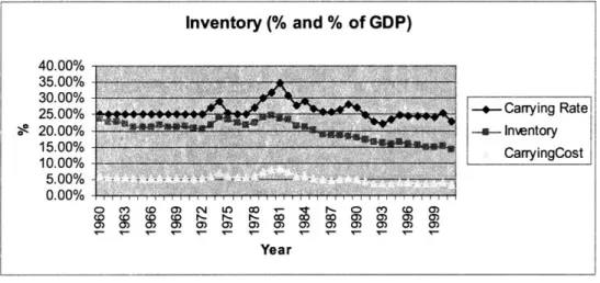
Inventory

The inventory carrying cost is the multiplication of inventory value and carrying rate of each year. The three components were quite stable in from 1960 to 1973. There were fluctuations from early 1970s to early 1990s. The three components were showing similar trend throughout the period as can be seen from Figure 2.

Inventory (% and % of GDP) 40.00% 35.00% 30.00% 25.00% -+- Carrying Rate e 20.00% 4- Invntory 15.00% -CarryingCost 10.00% 5.00%---0.00% o CY) CD 0) CN U) CD - I'- Q (C CD 0) CD WD CD CD I- I- I~- CO C O aD ) 0) 0) 0) Year

Figure 2: Inventory rate, level and cost as percentage of GDP

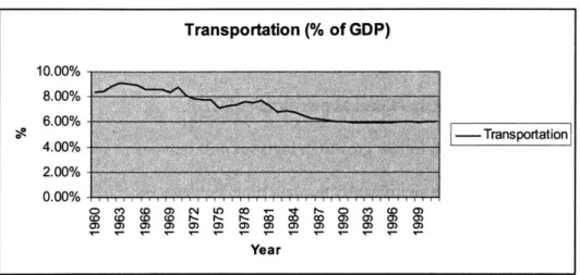
* Transportation

Transportation cost as percentage of GDP (Figure 3) showed decline from the beginning to the end. The cost swing up and down since 1960, not until 1990 that it has been flattened. The big decrease in percent of transportation cost occurred in 2 periods, 1970-1976 and 1981-1987.

Transportation (% of GDP) 10.00% 8.00% -. 00% - Transportation 2.00% 0.00% o CO CO O I LO~ CO F I- 0 (Vn CO O) CO CO (0 CO I'- I- I- CO o CoO 0) 0)M Year

Figure 3: Transportation cost as percentage of GDP

TFP

The residual of the rate of growth in labor and capital from the rate of growth in economy's output is so called TFP. TFP figures deriving from growth accounting method for US Economy from 1961-2001 are showed in Figure 4. TFP swing through time, however, TFP figures remained in the positive value most of the time, showing the overall increasing productivity trend.

Figure 4: Total Factor Productivity TFP 0.040% 0.030% 0.020% 0.010% 0.000% -0.0100% -0.020% -0.030% Year

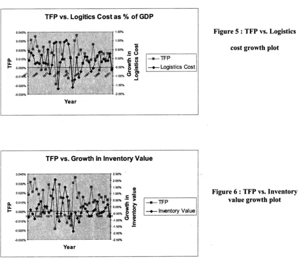
Comparison of TFP and Logistics cost.

As to compare to the rate of growth in productivity of the country, the analysis is based on the growth figure of cost as percentage of GDP.

TFP appeared to follow growth in logistics cost movement with some lag time. Both variables fluctuate significantly through time, however most of the time, both showed positive growth.

The comparison of TFP and logistics cost and other decompositions of logistics cost is shown in Figure 5 to Figure 9.

TFP vs. Logitics Cost as % of GDP

0.040% 71-50% 3 -0 F

0.00% 1 050% 0

0.000%o o -0. -- Logistics Cost

-0020% -150%

.030%

-Year

TFP vs. Growth in Inventory Value

0.040% 2.50%

0030%

U. _{000% 0}

L~~ ~ 9--050 OY* Inwentory Value

.0030% -2.50%

Year

Figure 5 : TFP vs. Logistics

cost growth plot

Figure 6: TFP vs. Inventory

TFP vs Growth in Carrying Rate

0.040% 4.00%

0.030% 3.00%

0.020%

100%

-Fv. rot -in-Carrying Rate

-0.010%ft

-3.00%

-0.020%

-u--0.030% -5.00%

Year

TFP vs. Growth in Carrying Cost

.. 030% 00%% 0.020%0 % 0.0% 0 - rnsotto I 0.010% -0 - -TFP -0.000%o- e CarryingCost -0.0% -0.010%j -0.020% .1.00% -0.03Y% - -1.50% Year

TFP vs. Growth in Transportation Cost

0.03 0% 0.40 0.020% 0.20% 0 S 0.010% o.00% i a TFP O.000% --0.20% o5 -+- Transportation -0.010% -0.40% -0.020% -0.60% } -0.030% .. a ..80% Year Figure 7: TFP vs. Carrying rate growth plot

Figure 8: TFP vs. Inventory carrying cost growth plot

Figure 9: TFP vs.

Transportation cost growth

Results

Regression analysis

The paper examined different assumption about the relationship of TFP and logistics cost. TFP is the dependent variable in the question, and logistics cost, inventory value, inventory carrying rate, inventory carrying cost and transportation cost are, individually, the independent variables of the analysis. The regression analyzed the correlation between TFP and each independent variable in 3 setups, no time lagged, 1 year time lagged and 2 year time lagged. The analysis assumed 95% confident interval. The simple linear relationship with different time-lag assumption of Y = a + bX, where Y is TFP, X is each independent variable is examined to see the relationship.

No Time Lagged

The regression result from the time series of TFP and each independent variable from 1961-2001 yielded mainly insignificant correlations, except for the hypothesis with inventory value as independent variable.

The regression showed the significant correlation between TFP and the growth in inventory value, the results obtained for interception and coefficient of the linear function are 9.596E-05 and -0.00992 respectively. P-value equaled 0.00024 showing significant correlation. The negative coefficients showed adverse relationship between productivity and growth in inventory level. The positive growth in inventory level will lead to lower productivity.

Adjusted R-square is approximately 0.3. The small figure is explained by the fact that TFP can be explained by many variable e.g. R&D, technology, and thus, does not solely depend upon the level of inventory in the economy.

1-year Time Lagged

In this hypothesis, we assume it will take 1 year for logistics efficiency to impact the productivity or where X at time t- 1 will affect Y at time t. The result from using TFP of one year period behind the independent variable yielded significant correlation in all of the factors, except transportation cost.

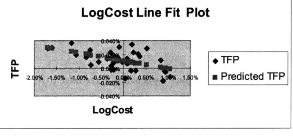
One-year lagged TFP and growth in logistics cost have negative coefficient of 0.01137 with the interception at 0.000104. The P-value is at 0.00039, thus showing that correlation is significant. The negative coefficient showed the lower logistics cost implying the higher efficiency in logistics activities will result in economy's higher productivity of the next year.

Similar results were obtained from each logistics factors as well. Each shows significant relationship. The inventory value has negative coefficient of -0.00989 and interception of 9.588E-05, implying one percentage change in proportion of inventory value in GDP will result in the change of TFP at 0.0095% in opposite direction. The coefficient for inventory carrying rate and carrying cost are -0.00572, and -0.01873 respectively. One-year time lagged model resulted in higher Adjusted R-square than those of other assumption, showing better fit of the equation. Among the factors, carrying cost appeared to have the relatively higher impact on TFP than other factors.

* 2-Year Time Lagged

This hypothesis assumes it will, instead, take 2 years for logistics efficiency to impact the productivity or where X at time t-2 will affect Y at time t. Similar to the no-lag analysis, there are not any significant correlation found between TFP and logistics cost and its components.

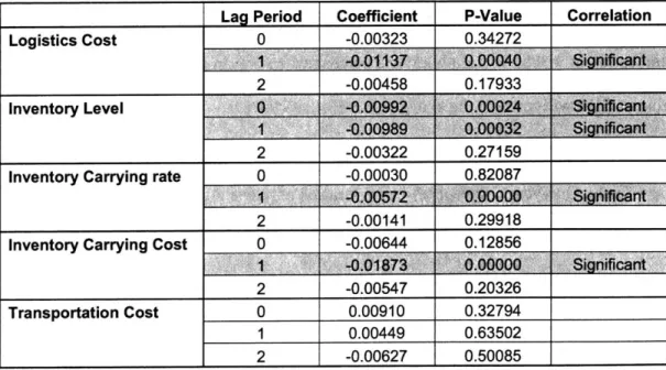
From the regression results, we can find significant correlation between productivity and logistics cost and its cost factors. Among the independent factors, growth in transportation cost is the only factor that does not shown any correlation to productivity. With significantly correlated factors, the R-square of each of them are small, this is due to the multi-factor contribution to TFP, mainly research and

development, technology, public policy, etc. Thus, logistics efficiency is not the sole determinant of TFP.

The summary of regression results for all the analysis is shown in Table 1.

Table I : Correlation of Growth in logistics cost factors and TFP

Lag Period Coefficient P-Value Correlation

Logistics Cost 0 -0.00323 0.34272

1 -9.011137 Q.00040 Sign!gw_.nt

2 -0.00458 0.17933

Inventory Level 0 0.0090 0.24cant

1 -0.00989 0.63502 ______S__nt

2 -0.00322 0.27159

Inventory Carrying rate 0 -0.00030 0.82087

1 -0.00572 &.99M igifcnt

2 -0.00141 0.29918

Inventory Carrying Cost 0 -0.00644 0.12856

1 -0.01873 O.00000 Significant

2 -0.00547 0.20326

Transportation Cost 0 0.00910 0.32794

1 0.00449 0.63502

Line Fit Plot Interpretation

The analysis will now focus on those results that are significantly correlated. One-year lagged model showed meaningful results for most of the independent variables,

while only inventory value showed the meaningful relationship for the no-lagged model. Byexaiining the line fit plot of the data in each model, we will identify the time periods that dictate the slope of the graph and strongly support the hypothesis in order to see whether or not we can find the common relationship among them.

* Logistics cost

The years with extreme combination in second quadrant of the line fit plot graph are 1975, 1982 and 1983 with series point of (0.028, -1.7), (0.030, -1.62) and (0.036,

-1.18) respectively. The combination in the forth quadrant are in year 1978-1980 with series points of (-0.004,-4.93), (-0.012, -0.04) and (-0.011, -0.83). (Figure 10)

LogCost Line Fit Plot

TFP

-2.6%--0 -100 0.50% OA 0 ti . Predicted TFP

LogCost

* Inventory Level Value

No time lagged

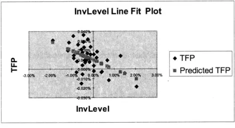
The regression resulted in the combination points at each edge of the downward sloping shape. Those plots with high productivity and low inventory level are 1976, 1983, and 1986 with the series of (0.028,-1.11), (0.030,-1.88) and (0.020,-1.17) respectively. Those that are in the opposite edge are in year 1974 and 1979 with series of (-0.019, 2.04)

and (-0.004, 1.48). (Figure 11)

InvLevel Line Fit Plot

+ * +TFP L - 2 0 0 Predicted TFP -3.UO% -2,M0% -1.OO 0 % 0 0% 3.C)% InvLevel

Figure 11: Growth in inventory level (no lag) and TFP line fit plot

1-year Time Lagged

In 1976, 1983 and 1985 showed the combination series of (0.015, -1.11), (0.036,-1.88%), and (0.020, -0.90). While in 1973, 1974 and 1979 showed the combination series of (-0.019, 1.13), (-0.006, 2.04), and (-0.012, 1.48). (Figure 12)

-.

InvLevel Line Fit Plot

+TFP

a Predicted TFP

.00 % .*% 3.00%

InvLevel

-3.

Figure 12 : Growth in Inventory level (lagi) and TFP line fit plot

Inventory Carrying Rate

Carrying rate and productivity has strong adverse relationship in 1975, 1982, and 1983 with combination points of (-0.019, 2.20), (-0.012, 3.0) and (-0.0 15, 2.9) as well as in 1973, 1979, 1981 with combination points of (0.028,-3.70), (0.030,-3.90), and (0.036,-2.90). (Figure 13)

0. U-

I-Carrying Rate Line Fit Plot

+ d*TFP

n Predicted TFP

Carrying Rate

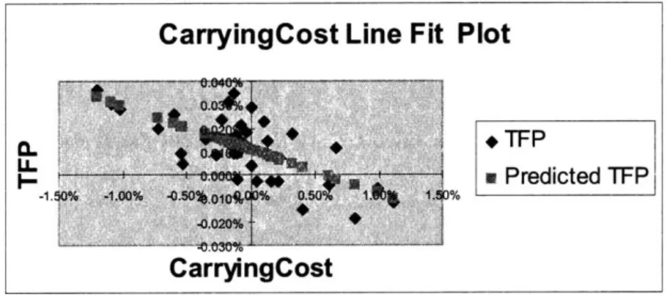
* Inventory Carry cost

In 1975, 1982 and 1983 showed the combination series of (0.028, -1.01), (0.030,-1.10%), and (0.036, -1.20). While in 1973, 1974 and 1979 showed the combination series of (-0.019, 0.81), (-0.006, 0.99), and (-0.012, 1.12). (Figure 14)

CarryingCost Line Fit Plot

CI+ TFP

. Predicted TFP

-0.020%

CarryingCost

Figure 14 : Growth in Carrying cost and TFP line fit plot

Summary

Each line fit plot exhibited similar characteristics. While most of the data are more scattered in the middle in less significantly correlated fashion, those at the tails are more concentrated around the predicted value, and are fewer in number.

Interestingly, the time period that we find strong adverse relationship between productivity and each independent variable are very similar. Those periods are 1975,

1976, and 1982-1986 for the combination with negative productivity and 1973, 1974, and 1978-1981 for the combination with positive productivity. The two scenarios combined resulted in the consecutive years of amplified relationship from 1973 to 1986.

Figure 15 : Logistics cost and its factor movement in 1973-1986

From Figure 15, the period in question of 1973-1986 commonly, among dependent variables, showed substantial fluctuation of its percentage and percentage of GDP. The fluctuation in this period is significant and markedly higher than any other period in the study. This possibly suggested that in the period where the efficiency of logistics abruptly changes, it affected significantly the economy's productivity and the negative correlation is clear.

Other concurrent events in the history in those periods are the recession of 1974-1975 and the deregulation of transportation industry in early 1980s. Recession forced businesses to be more efficient and cost effective in their production, logistics operations were forced to become higher in productivity, while the transition period to the

deregulated trucking industry slowed down the efficiency in logistics industry as a whole. These situations explained the efficiency and inefficiency of the operations that might not be explicitly represented in the logistics cost.

Logistics and its factor cost ( % and % of GDP) 1973-1986 40.00% -35.00% 30.00%-25.00% 8 20.00% 15.00% -10.00% 5.00% -0.00% Year -+- Carrying Rate w- Inventory CarryingCost Logistics Cost

Chapter 4

Conclusion and Recommendations

Conclusion

The study found significant correlation between 4 independent variables, which are logistics cost, inventory level, inventory carrying rate, and inventory carrying cost, and TFP. There was no correlation between transportation cost and TFP. Among those significant correlations, all were correlated to TFP with one year lagged time, meaning the movement of the independent in 1990 correlated with the movement of TFP in 1991, except for inventory level which were significantly correlated to both TFP of the same year and TFP of one year lagged. R-square of each regression are about 0.3 for logistics cost and about 0.5 for inventory factors, implying that neither logistics cost nor inventory factor are the sole determining factor of productivity.

All significant correlations showed negative sign of coefficient indicating the adverse relationship between its growth and TFP. The higher the growth of each

independent variable, namely logistics cost, inventory level, inventory carrying rate, and inventory carrying cost is, the lower the development of productivity in the economy of the next year.

Among them, inventory carrying cost at one-year lagged has the biggest value of coefficient at -0.01873%, while logistics cost has the second biggest coefficient value of

- 0.1137%, inventory level with no lagged and with one year lagged have similar coefficient value of about 0.0099% and inventory carrying rate's coefficient is at

Logistics cost is the sum of inventory carrying cost and transportation cost, while inventory carrying cost itself is the product of inventory level and carrying rate. This suggests that efficiency in inventory management from lowering inventory level in the economy and/or reducing the carrying rate by efficiently manage those controllable factors such as warehousing cost and obsolescence cost would correlated to the better productivity figure of the economy in the year after.

The study of line fit plot graph yielded interesting findings. In 1973 to 1986 were the time period that we find strong adverse relationship between productivity and each independent variable presented in each tail of line fit plot graph. In this period, the growth's fluctuation of each independent variable is markedly higher than any other period in the study. This possibly suggested the abrupt changes in logistics efficiency might affect significantly to economy's productivity than the regular periods.

Listed in the history of this period are the recession of 1974-1975 and the deregulation of transportation industry in early 1980s. Recession forced every business unit including logistics operations to become more efficient, while the struggle from deregulation transition slowed down the efficiency in logistics industry as a whole. These situations explained the qualitative efficiency and inefficiency of the operations that might not be incorporated into the calculation of quantitative efficiency determine by logistics cost, but contribute to the stronger correlation with productivity.

Though causality of these factors cannot be concluded, significant correlation between them presents interesting links between the relationship of micro-level logistics and macro-level concept of productivity.

Recommendations

Further study can explore the causality relationship between logistics cost and productivity. Qualitative part of efficiency in logistics management is also interesting and critical to take into consideration. Reduction in logistics cost as percentage of GDP is a reasonable measurement of logistics activities, but there are other aspects beyond that. The goal of logistics management is not merely cost minimization but, instead, cost minimization given the desired service level. Thus, it might not be fair to conclude that the growth in logistics cost as percentage of GDP is the symptom of logistics inefficiency if the service level improvement achieved at that period were significantly higher than it would have been without efficiency.

Another interesting study is to identify the importance of logistics activities to the growth of the developing country. In many developing countries, the concept of logistics is still very new. The message is better conveyed to and receives more attention from public using familiar concepts. However, two major challenges in the study would be whether the necessary data will already be collected, and how far back the data are available. This is to identify logistics as the source of competitive advantage and the sustainable growth of the developing country where the government takes more aggressive role in term of development. Rarely is there any research done on how the activities in the real sector down to plant level contribute to productivity growth. Thus, the study of this area should facilitate the formulating of public policy and budget toward

Appendix

Estimation ofLogistics costs as percentage of GDP (State of Logistics Report 2002) Year Inventory Carrying Cost Transportation Administration Logistics

1960 23.70% 5.93% 8.34% 0.57% 14.84% 1961 22.91% 5.75% 8.43% 0.55% 14.73% 1962 22.68% 5.67% 8.87% 0.51% 15.05% 1963 22.14% 5.54% 9.05% 0.65% 15.23% 1964 21.22% 5.31% 9.03% 0.60% 14.94% 1965 21.11% 5.28% 8.89% 0.56% 14.72% 1966 21.28% 5.32% 8.62% 0.51% 14.44% 1967 21.70% 5.43% 8.63% 0.60% 14.66% 1968 21.28% 5.32% 8.56% 0.55% 14.43% 1969 21.31% 5.33% 8.32% 0.51% 14.16% 1970 21.35% 5.34% 8.75% 0.58% 14.67% 1971 20.91% 5.23% 8.06% 0.53% 13.82% 1972 20.64% 5.16% 7.82% 0.48% 13.46% 1973 21.94% 5.97% 7.80% 0.58% 14.34% 1974 23.98% 6.96% 7.73% 0.60% 15.28% 1975 23.48% 5.94% 7.09% 0.55% 13.59% 1976 22.37% 5.59% 7.29% 0.49% 13.38% 1977 21.86% 5.46% 7.38% 0.49% 13.34% 1978 22.52% 6.08% 7.62% 0.57% 14.27% 1979 24.00% 7.20% 7.52% 0.58% 15.31% 1980 24.75% 7.87% 7.65% 0.61% 16.13% 1981 23.86% 8.28% 7.28% 0.61% 16.17% 1982 23.32% 7.18% 6.81% 0.55% 14.55% 1983 21.44% 5.98% 6.87% 0.51% 13.37% 1984 21.00% 6.11% 6.81% 0.51% 13.44% 1985 20.10% 5.39% 6.50% 0.47% 12.37% 1986 18.93% 4.87% 6.31% 0.45% 11.63% 1987 18.45% 4.74% 6.20% 0.44% 11.38% 1988 18.48% 4.92% 6.13% 0.45% 11.49% 1989 18.31% 5.14% 5.99% 0.44% 11.58% 1990 17.94% 4.88% 6.05% 0.43% 11.36% 1991 17.21% 4.28% 5.93% 0.40% 10.62% 1992 16.51% 3.75% 5.93% 0.38% 10.06% 1993 16.20% 3.60% 5.96% 0.38% 9.93% 1994 15.98% 3.75% 5.95% 0.38% 10.09% 1995 16.36% 4.07% 5.96% 0.41% 10.44% 1996 15.87% 3.87% 5.98% 0.40% 10.25% 1997 15.39% 3.77% 6.05% 0.40% 10.21% 1998 15.00% 3.66% 6.02% 0.39% 10.07% 1999 14.89% 3.59% 5.97% 0.38% 9.94% 2000 15.04% 3.81% 6.01% 0.40% 10.21% 2001 14.28% 3.26% 6.00% 0.37% 9.62%

Estimation of TFP using Growth Accounting Method

Year LN(Qt/Qt-1) LN(Lt/L LN(K-Kt-1) Ave.L share Ave.K share TFP

1960 _ 1961 0.023 -0.001 0.019 0.692 0.308 0.018% 1962 0.059 0.030 0.022 0.688 0.312 0.031% 1963 0.042 0.017 0.032 0.685 0.315 0.021% 1964 0.056 0.023 0.019 0.684 0.316 0.035% 1965 0.062 0.038 0.040 0.681 0.319 0.023% 1966 0.064 0.049 0.038 0.681 0.319 0.018% 1967 0.025 0.016 0.052 0.691 0.309 -0.003% 1968 0.047 0.022 0.029 0.701 0.299 0.023% 1969 0.030 0.028 0.043 0.712 0.288 -0.002% 1970 0.002 -0.016 0.035 0.728 0.272 0.004% 1971 0.033 -0.006 0.032 0.733 0.267 0.029% 1972 0.053 0.029 0.056 0.727 0.273 0.017% 1973 0.056 0.042 0.043 0.722 0.278 0.014% 1974 -0.006 0.002 0.043 0.727 0.273 -0.019% 1975 -0.004 -0.028 0.083 0.732 0.268 -0.006% 1976 0.054 0.028 0.019 0.728 0.272 0.028% 1977 0.045 0.033 0.024 0.724 0.276 0.015% 1978 0.054 0.046 0.042 0.720 0.280 0.009% 1979 0.031 0.032 0.046 0.721 0.279 -0.004% 1980 -0.002 -0.008 0.057 0.730 0.270 -0.012% 1981 0.024 0.004 0.039 0.734 0.266 0.011% 1982 -0.020 -0.020 0.034 0.736 0.264 -0.015% 1983 0.042 0.013 0.010 0.735 0.265 0.030% 1984 0.070 0.049 -0.005 0.722 0.278 0.036% 1985 0.038 0.024 0.024 0.715 0.285 0.014% 1986 0.034 0.009 0.026 0.723 0.277 0.020% 1987 0.033 0.030 0.026 0.727 0.273 0.004% 1988 0.041 0.027 0.022 0.720 0.280 0.015% 1989 0.034 0.029 0.022 0.717 0.283 0.008% 1990 0.017 0.009 0.016 0.720 0.280 0.007% 1991 -0.005 -0.022 0.010 0.724 0.276 0.008% 1992 0.030 0.007 -0.004 0.728 0.272 0.026% 1993 0.026 0.017 0.017 0.728 0.272 0.009% 1994 0.040 0.027 0.030 0.725 0.275 0.012% 1995 0.026 0.026 0.038 0.719 0.281 -0.003% 1996 0.035 0.014 0.027 0.711 0.289 0.017% 1997 0.043 0.029 0.027 0.705 0.295 0.015% 1998 0.042 0.030 0.039 0.706 0.294 0.009% 1999 0.040 0.020 0.036 0.710 0.290 0.016% 2000 0.037 0.018 0.041 0.714 0.286 0.012% 2001 0.003 -0.008 0.041 0.720 0.280 -0.003%

Summary of Regression Results

Logistics cost

Y TFP

K Change in Logistics cost in % of GDP

Y(t)= A+BX(t) Regression Statistics Multiple R 0.152016385 R Square 0.023108981 Adjusted R Square -0.001939506 Standard Error 0.000132517 Observations 41 ANOVA df SS MS F Significance F

Regression 1 1.6201 E-08 1.6201 E-08 0.922569919 0.342718552

Residual 39 6.84867E-07 1.75607E-08

Total 40 7.01068E-07

Coefficients Standard Error t Stat P-value Lower 95% Upper 95%

Intercept 0.00011466 2.11327E-05 5.425714789 3.24445E-06 7.19152E-05 0.000157405

LogCost -0.003230213 0.003363035 -0.960505033 0.342718552 -0.010032587 0.003572162 Y(t) = A+BX(t-1) Regression Statistics Multiple R 0.532960325 R Square 0.284046709 Adjusted R Square 0.265205832 Standard Error 0.000114634 Observations 40 ANOVA df SS MS F Significance F

Regression 1 1.98114E-07 1.98114E-07 15.07608814 0.000399182

Residual 38 4.99357E-07 1.3141E-08

Total 39 6.97471E-07

Coefficients Standard Error t Stat P-value Lower 95% Upper 95%

Intercept 0.000104124 1.84395E-05 5.646807204 1.73731 E-06 6.67955E-05 0.000141453

Y(t) = A+BX(t-2) Regression Statistics Multiple R 0.219531839 R Square 0.048194228 Adjusted R Square 0.022469748 Standard Error 0.000130155 Observations 39 ANOVA df SS MS F Significance F

Regression 1 3.17373E-08 3.17373E-08 1.87347724 0.179330675

Residual 37 6.26792E-07 1.69403E-08

Total 38 6.5853E-07

Coefficients Standard Error t Stat P-value Lower 95% Upper 95%

Intercept 0.000106544 2.126E-05 5.011499475 1.36135E-05 6.34677E-05 0.000149621

Inventory Level

TFP

Growth in inventory value as % of GDP Y(t)= A+BX(t) Regression Statistics Multiple R 0.543984304 R Square 0.295918923 Adjusted R Square 0.277865562 Standard Error 0.000112502 Observations 41 ANOVA df SS MS F Significance F

Regression 1 2.07459E-07 2.07459E-07 16.39134807 0.000236735

Residual 39 4.93609E-07 1.26566E-08

Total 40 7.01068E-07

Standard

Coefficients Error t Stat P-value Lower 95% Upper 95%

Intercept 9.5985E-05 1.84489E-05 5.202743029 6.59315E-06 5.86686E-05 0.000133301

InvLevel -0.009917286 0.002449546 -4.048622984 0.000236735 -0.014871955 -0.004962618 Y(t) = A+BX(t-1) Regression Statistics Multiple R 0.529049288 R Square 0.279893149 Adjusted R Square 0.260430802 Standard Error 0.00011321 Observations 39 ANOVA df SS MS F Significance F

Regression 1 1.84318E-07 1.84318E-07 14.38126373 0.000534698

Residual 37 4.74212E-07 1.28165E-08

Total 38 6.5853E-07

Standard

Coefficients Error t Stat P-value Lower 95% Upper 95%

Intercept 9.58803E-05 1.88215E-05 5.094176911 1.64341E-05 5.50281E-05 0.000131283

InvLevel -0.009890335 0.002502793 -3.792263668 0.000534698 -0.014562385 -0.004420115

Y x

Y(t) = A+BX(t-2) Regression Statistics Multiple R 0.180467303 R Square 0.032568448 Adjusted R Square 0.006421649 Standard Error 0.000131219 Observations 39 ANOVA df SS MS F Significance F

Regression 1 2.14473E-08 2.14473E-08 1.245599811 0.271590524

Residual 37 6.37082E-07 1.72184E-08

Total 38 6.5853E-07

Standard

Coefficients Error t Stat P-value Lower 95% Upper 95%

Intercept 0.000105012 2.20006E-05 4.773137202 2.83714E-05 6.04344E-05 0.000149589

Inventory Carrying Rate

Y TFP

X Growth in carrying rate

Y(t)= A+BX(t) Regression Statistics Multiple R 0.036477382 R Square 0.001330599 Adjusted R Square -0.024276308 Standard Error 0.000133986 Observations 41 ANOVA df SS MS F Significance F

Regression 1 9.32841E-10 9.32841E-10 0.051962518 0.820873798

Residual 39 7.00135E-07 1.79522E-08

Total 40 7.01068E-07

Standard

Coefficients Error t Stat P-value Lower 95% Upper 95%

Intercept 0.000118606 2.09369E-05 5.66493458 1.5121 E-06 7.62575E-05 0.000160955

Carrying Rate -0.000299606 0.001314332 -0.227952886 0.820873798 -0.00295809 0.002358879 Y(t) = A+BX(t-1) Regression Statistics Multiple R 0.676755816 R Square 0.457998434 Adjusted R Square 0.443735235

Standard Error 9.97405E-05

Observations 40

ANOVA

df SS MS F Significance F

Regression 1 3.19441 E-07 3.19441 E-07 32.11049859 1.63199E-06

Residual 38 3.7803E-07 9.94817E-09

Total 39 6.97471E-07

Standard

Coefficients Error t Stat P-value Lower 95% Upper 95%

Intercept 0.000117715 1.57705E-05 7.46422489 5.84155E-09 8.57891 E-05 0.000149641

Y(t) = A+BX(t-2) Regression Statistics Multiple R 0.170571011 R Square 0.02909447 Adjusted R Square 0.00285378 Standard Error 0.000131454 Observations 39 ANOVA df SS MS F Significance F

Regression 1 1.91596E-08 1.91596E-08 1.108753992 0.299181203

Residual 37 6.3937E-07 1.72803E-08

Total 38 6.5853E-07

Standard

Coefficients Error t Stat P-value Lower 95% Upper 95%

Intercept 0.000111965 2.10518E-05 5.318516833 5.25354E-06 6.93095E-05 0.00015462

Inventory Carrying Cost

TFP

Growth in Inventory Carrying Cost as percentage of GDP Y(t)= A+BX(t) Regression Statistics Multiple R 0.241293032 R Square 0.058222327 Adjusted R Square 0.034074182 Standard Error 0.000130113 Observations 41 ANOVA df SS MS F Significance F

Regression 1 4.08178E-08 4.08178E-08 2.411047557 0.128559978

Residual 39 6.6025E-07 1.69295E-08

Total 40 7.01068E-07

Standard

Coefficients Error t Stat P-value Lower 95% Upper 95%

Intercept 0.000114578 2.04986E-05 5.589531162 1.92392E-06 7.31154E-05 0.00015604

CarryingCost -0.006435936 0.00414485 -1.552754828 0.128559978 -0.014819679 0.001947806 Y(t) = A+BX(t-1) Regression Statistics Multiple R 0.695266664 R Square 0.483395735 Adjusted R Square 0.469800886

Standard Error 9.73756E-05

Observations 40

ANOVA

df SS MS F Significance F

Regression 1 3.37155E-07 3.37155E-07 35.55727111 6.39874E-07

Residual 38 3.60317E-07 9.48201 E-09

Total 39 6.97471E-07

Standard

Coefficients Error t Stat P-value Lower 95% Upper 95%

Intercept 0.000107365 1.54861 E-05 6.932972901 3.03075E-08 7.60147E-05 0.000138715

CarryingCost -0.018727111 0.003140556 -5.962991792 6.39874E-07 -0.025084836 -0.012369387

Y

Y(t) = A+BX(t-2) Regression Statistics Multiple R 0.208268969 R Square 0.043375963 Adjusted R Square 0.01752126 Standard Error 0.000130484 Observations 39 ANOVA df SS MS F Significance F

Regression 1 2.85644E-08 2.85644E-08 1.677681707 0.203256446

Residual 37 6.29965E-07 1.70261E-08

Total 38 6.5853E-07

Standard

Coefficients Error t Stat P-value Lower 95% Upper 95%

Intercept 0.000109011 2.10469E-05 5.179434225 8.09255E-06 6.63662E-05 0.000151656

Transportation Cost

TFP

Growth in Transportation Cost as percentage of GDP Y(t)= A+BX(t) Regression Statistics Multiple R 0.156678091 R Square 0.024548024 Adjusted R Square -0.000463565 Standard Error 0.000132419 Observations 41 ANOVA df SS MS F Significance F

Regression 1 1.72098E-08 1.72098E-08 0.981465999 0.327944165

Residual 39 6.83858E-07 1.75348E-08

Total 40 7.01068E-07

Standard

Coefficients Error t Stat P-value Lower 95% Upper 95%

Intercept 0.000123965 2.13355E-05 5.810257726 9.5021E-07 8.08096E-05 0.00016712

transport 0.009098486 0.009183992 0.990689658 0.327944165 -0.009477873 0.027674844 Y(t) = A+BX(t-1) Regression Statistics 0 Multiple R 0.077394955 R Square 0.005989979 Adjusted R Square -0.020168179 Standard Error 0.000135072 Observations 40 ANOVA 0 0 df SS MS F Significance F

Regression 1 4.17784E-09 4.17784E-09 0.228990857 0.635015013

Residual 38 6.93293E-07 1.82446E-08

Total 39 6.97471E-07

Standard

Coefficients Error t Stat P-value Lower 95% Upper 95%

Intercept 0.000119908 2.20482E-05 5.43842928 3.35247E-06 7.52734E-05 0.000164542

transport 0.004485919 0.009374376 0.478529892 0.635015013 -0.014491513 0.023463351

Y

Y(t) = A+BX(t-2) Regression Statistics Multiple R 0.111070221 R Square 0.012336594 Adjusted R -Square 0.014357011 Standard Error 0.000132584 Observations 39 ANOVA df SS MS F Significance F

Regression 1 8.12401 E-09 8.12401 E-09 0.462155405 0.50084987

Residual 37 6.50406E-07 1.75785E-08

Total 38 6.5853E-07

Standard

Coefficients Error t Stat P-value Lower 95% Upper 95%

Intercept 0.000108482 2.1957E-05 4.940664923 1.69424E-05 6.3993E-05 0.000152971

Bibliography

Acemoglu, Daron. TFP differences! Cambridge, Mass. : Massachusetts Institute of Technology, [1998]

Arrow, Kenneth Joseph, 1921- Total factor productivity growth in individual industries and in the economy, Cambridge, Mass., Harvard University, Center for International Affairs, Project for Quantitative Research in Economic Development, 1969.

Demirjian, Ara Manuel. Total factor productivity movements in the air transportation industry from 1965 to 1980 / c1983.

Felipe, Jesus. Total factor productivity growth in East Asia : a critical survey / Manila, Philippines: Asian Development Bank, c1997.

Hammer, Michael, 1948- The agenda: what every business must do to dominate the decade / New York: Crown Business, c2001.

Heskett, Ivie and Glaskowsky. Business Logistics / New York: The Ronal Press Company., 1973.

Hulten, Chalres R. Total Factor Productivity: A Short Bibliography/ NBER Working paper No. 7471 (2000)

Krugman, Paul R., The Myth of Asia's Miracle / Foreign Affairs, November-December: 62-78 (1994)

Mamgain, Vaishali. Productivity growth in developing countries : the role of efficiency

/ New York: Garland Pub., 2000.

Nishimizu, M. and J.M. Page. Total factor productivity growth, technological progress and technical efficiency change: Dimensions of productivity change in Yugoslavia, 1965-1978 / Economic Journal 92 (1982): 920-36

Production handbook, New York, Ronald Press Co., 1958.

Shimizu, Toshihiko. Valuation capacity and measures of total factor productivity : a case study of the Tokyo Electric Power Company, Inc. / c1985.

Smith, Frank A. (Frank Albert), 1922- Transportation in America : a statistical analysis of transportation in the United States : historical compendium, 1939-1985 / Westport, CT

: Eno Foundation for Transportation, 1989.

Tinakorn P. and Sussangkarn C. Productivity Growth in Thailand/ TDRI Quarterly Review Vol.9 No.4 December 1994: 35-40

Young, Alwyn. The Tyranny of Numbers: Confronting the Statistical Realities of the East Asian Growth Experience / NBER Working paper No. 4680 (1994)

Internet Documents

Robert V. Delaney's 12th Annual State of Logistics Report from

http://www.cassinfo.com/2001%20Press%20Conference%2OFinal.PDF, March 2003 Robert V. Delaney's 13th Annual State of Logistics Report from

http://www.cassinfo.com/2002%20Press%20Conference%20Full.pdf, March 2003 Contribution of Highway Capital to Output and Productivity Growth from