HAL Id: hal-02136451
https://hal.archives-ouvertes.fr/hal-02136451
Submitted on 22 May 2019HAL is a multi-disciplinary open access
archive for the deposit and dissemination of
sci-L’archive ouverte pluridisciplinaire HAL, est destinée au dépôt et à la diffusion de documents
Residual-Mean Circulation
F. Sevellec, A. Naveira Garabato, C. Vic, N. Ducousso
To cite this version:
F. Sevellec, A. Naveira Garabato, C. Vic, N. Ducousso. Observing the Local Emergence of the Southern Ocean Residual-Mean Circulation. Geophysical Research Letters, American Geophysical Union, 2019, 46 (7), pp.3862-3870. �10.1029/2018GL081382�. �hal-02136451�
Observing the Local Emergence of the Southern
1Ocean Residual-Mean Circulation
2F. S´evellec1,2, A. Naveira Garabato2, C. Vic2, and N. Ducousso1
1Laboratoire d’Oc´eanographie Physique
et Spatiale, CNRS Univ.-Brest IRD Ifremer, Brest, France
2Ocean and Earth Science, University of
Key Points.
◦ Horizontal buoyancy advection by mesoscale eddies at a Southern Ocean mooring site balances mean vertical advection on timescale of 100 days.
◦ The overturning circulation of the South-ern Ocean emerges on this timescale as a residual between the eddy-induced and Eulerian-mean flows.
◦ The eddy-induced flow can be accurately parameterized with a Gent-McWilliams diffusivity of ∼2,000 m2 s−1.
Abstract
3
The role of mesoscale turbulence in
maintain-4
ing the mean buoyancy structure and
overturn-5
ing circulation of the Southern Ocean is
in-6
vestigated through a 2-year-long, single-mooring
7
record of measurements in Drake Passage. The
8
buoyancy budget of the area is successively
9
assessed within the Eulerian and the
Temporal-10
Residual-Mean frameworks. We find that a regime
11
change occurs on timescales of 1 day to 100 days,
12
characteristic of mesoscale dynamics, whereby
13
the eddy-induced turbulent horizontal
tion balances the vertical buoyancy advection
15
by the mean flow. We use these diagnostics
16
to reconstruct the region’s overturning
circu-17
lation, which is found to entail an equatorward
18
downwelling of Antarctic Intermediate and
Bot-19
tom Waters and a poleward upwelling of
Cir-20
cumpolar Deep Water. The estimated
eddy-21
induced flow can be accurately parameterized
22
via the Gent-McWilliams closure by
adopt-23
ing a diffusivity of ∼2,000 m2 s−1 with a
mid-24
depth increase to 2,500 m2 s−1 at 2,100 m,
im-25
mediately underneath the maximum interior
26
stratification.
1. Introduction
The Southern Ocean plays a pivotal role in the global ocean circulation by connecting
28
the Indian, Pacific, and Atlantic basins [Schmitz , 1996], and the ocean’s deep and surface
29
layers [Lumpkin and Speer , 2007]. The regional circulation is shaped by physical processes
30
acting on a wide range of spatio-temporal scales – from large-scale, persistent Ekman flows,
31
directly linked to surface wind forcing, to meso- and small-scale turbulent motions [Speer
32
et al., 2000]. Assessing the relative contributions of, and interplay between, this spectrum
33
of flows in determining the Southern Ocean limb of the Meridional Overturning Circulation
34
(MOC) remains an important open question, with implications for e.g., global ocean heat
35
uptake [Liu et al., 2018] and sequestration of carbon dioxide [Landsch¨utzer et al., 2015].
36
However, a complete assessment of these dynamics and their effects is outstanding due to
37
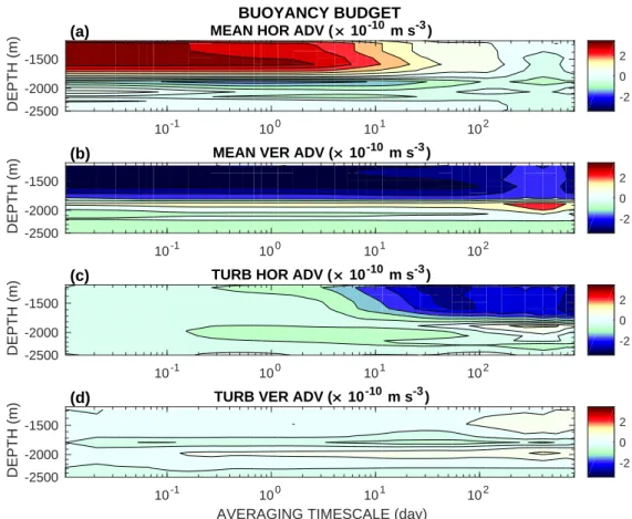
the difficulty of rigorously distinguishing between averaged quantities (produced through
38
inaccurate diagnostic) and mixed quantities (produced through actual mixing). Averaged
39
quantities can be likened to the development of a blurred picture in photography when
40
an overly long exposure time is used to capture a moving object. Hence, unlike mixed
41
quantities, they are the outcome of an inaccurate observation rather than a property
42
of the observed system. The erroneous interpretation of averaged quantities as mixed
43
quantities has been rationalized in the context of the time-mean ocean circulation through
44
the Temporal-Residual-Mean (TRM) framework put forward by McDougall and McIntosh
45
[2001].
46
Here, we acknowledge this issue, by examining and quantifying the way in which the
47
mean buoyancy structure and overturning circulation are established at a Southern Ocean
site, where a mooring was deployed for 2 years. This also allows us to estimate the
eddy-49
induced Gent-McWilliams diffusivities. To conclude, a discussion of the impact of our
50
observational results for our understanding and numerical model representation of the
51
Southern Ocean limb of the MOC is provided.
52
2. Two distinct buoyancy budget regimes
To assess the contributions of motions of different scales to sustaining the extension of
53
the MOC across the Southern Ocean, we used in situ observations from a mooring located
54
in the Antarctic Circumpolar Current (ACC) at 56◦S, 57◦50′W (Fig. 1a), leeward of the
55
Drake Passage [see Fig. 1a and Brearley et al., 2013, for details of the exact location].
56
These 2-year long measurements were part of a 6-mooring cluster deployed under the
aus-57
pices of the Diapycnal and Isopycnal Mixing Experiment in the Southern Ocean [DIMES,
58
Naveira Garabato, 2010; Meredith, 2011]. This study uses co-located horizonal velocity,
59
temperature, salinity and pressure data at 1200-, 1299-, 1853-, 1951-, 2049-, 2152-, 3400-,
60
3600-m depth (see Text S1 for further details). From these observations, vertical velocities
61
can be inferred, and the terms of a time-mean buoyancy budget can be diagnosed. The
62
method to compute vertical velocities from single-mooring measurements is described in
63
S´evellec et al.[2015] and summarized in Text S2; the mean statistical properties of the
ob-64
servational record are shown in Figs. 1b-g. Taking advantage of the equivalent-barotropic
65
nature of the ACC flow [Killworth and Hughes, 2002], we defined gradients in the along
66
and across directions of the time- and depth-mean flow (as indicated in Fig. 1a). This
67
enables us to eliminate contributions to the buoyancy budget from the time-mean flow in
68
the across direction (Fig. 1c), except for a small baroclinic component.
Since the measurements were obtained at broadly constant depth levels, it is natural
70
to compute the buoyancy balance in an Eulerian framework with fixed depths. We start
71
from the buoyancy conservation equation:
72
∂tb+ u∂xb+ v∂yb+ w∂zb = 0, (1)
where t is time; x, y, and z are the along, across, and vertical directions; b is the buoyancy;
73
and u, v, and w are the along, across, and vertical velocities. By applying a Reynolds
74
decomposition, set for a range of averaging periods (from 15 minutes to ∼2 years), we
75
separate mean quantities from fluctuations. Taking the overall long-time-mean of this
76
decomposition allows us to build a mean buoyancy budget, which intrinsically depends on
77
the averaging/filtering period (as described in Text S3). This can be expressed in terms
78
of mean and turbulent advection as:
79
Meanhor(τ, z) + Meanver(τ, z) ≃ Turbhor(τ, z) + Turbver(τ, z), (2) where τ is the averaging period, Meanhor and Meanverare the mean horizontal and vertical
80
advection of buoyancy, and Turbhor and Turbver are the turbulent horizontal and vertical
81
advection of buoyancy, respectively. The mean buoyancy budget measures the relative
82
contribution of the turbulent/fluctuation and mean terms in setting the long-time-mean
83
equilibrium. It also shows how these contributions depend on the averaging/filtering
84
period used in the Reynolds decomposition. Note that there is also a trend term in (??)
85
compared to (2); however, it is negligible at all depths and for all averaging timescales by
86
construction of the mean buoyancy budget (Text S3).
The resulting buoyancy advective terms are enhanced in the upper part of the measured
88
water column, between 1,000 m and 2,000 m (Fig. 2), where buoyancy gradients, and
89
notably vertical stratification, attain maximum values (Fig. 1). The turbulent vertical
90
advection (Fig. 2d) is negligible at all depths and for all averaging periods. This indicates
91
that variations in vertical velocity and vertical stratification do not correlate highly enough
92
to sustain a net turbulent advection, despite their substantial magnitudes compared to
93
their mean values (Figs. 1d and 1g). In contrast, the mean vertical advection induces a
94
buoyancy gain between 1,000 m and 2,000 m (Fig. 2b). This is consistent with a mean
95
downwelling of buoyant water: a downward mean vertical velocity through a positive
96
vertical stratification. The mean downwelling is robust to changes in averaging period,
97
confirming the steadiness of this buoyancy flux.
98
The mean horizontal advection induces a buoyancy loss between 1,000 m and 2,000 m
99
for averaging periods shorter than 1 day, but is insignificant for periods longer than
100
∼100 days (Fig. 2a). This dependency to averaging timescale suggests that this term
101
is not sustained by a steady horizontal flow. Finally, the turbulent horizontal advection
102
also induces a buoyancy loss between 1,000 m and 2,000 m (Fig. 2c) that emerges for
103
averaging periods longer than ∼1 day, converging to a steady value for periods longer
104
than 100 days. This indicates that variations in horizontal velocity (Fig. 1b and 1c) and
105
in horizontal buoyancy gradients (Fig. 1e and 1f) are significantly correlated on periods
106
between 1 day and 100 days.
107
The preceding Eulerian buoyancy budget exhibits a remarkable dependence on
averag-108
ing period. Whereas on short timescales the buoyancy balance is between the mean
horizontal advection and the mean vertical advection (Meanhor+Meanver≃0), on long
110
timescales it is the turbulent horizontal advection that balances the mean vertical
advec-111
tion (Meanver≃Turbhor). The change in regime occurs between 1-100 days. This timescale
112
is characteristic of mesoscale dynamics, as may be shown e.g., by considering the 6-day
113
propagation timescale derived from the observed zonal propagation speed of mesoscale
114
eddies [2 cm s−1, Klocker and Marshall , 2014] and the baroclinic Rossby deformation
115
radius [10 km, Chelton et al., 1998] characteristic of the ACC. Accordingly, variability
116
within this timescale will be referred to as mesoscale turbulence in the remainder of this
117
study [Klocker and Abernathey, 2014].
118
The permanent regime is reached for averaging periods of 100 days. This convergence
119
timescale was reported by S´evellec et al. [2015] in a previous investigation of regional
120
dynamics. This period is linked to the cumulative effect of mesoscale eddies propagating
121
over the mooring site, and defines the minimum time over which measurements of eddy
122
variables must be acquired to obtain robust statistics and a convergence of the buoyancy
123
budget. This is symptomatic of the central role of eddies in sustaining the turbulent
124
horizontal advection. On timescales of 100 days, a balance is established between mean
125
vertical advection leading to a buoyancy gain and turbulent horizontal advection inducing
126
a buoyancy loss, in the depth range between 1,000 m and 2,000 m (Fig 2). This is
con-127
sistent with the prevalent view of the Southern Ocean limb of the MOC equatorward of
128
the ACC’s axis, where the mooring is located (i.e., equatorward of the maximum gradient
129
of dynamic ocean topography, Fig.1a). In this area, buoyant waters are expected to be
130
downwelled by the mean vertical circulation; this effect is balanced by the mesoscale
dies inducing a sink of buoyancy at depth [Toggweiler and Samuels, 1995, 1998; Marshall
132
and Radko, 2003, 2006]. If ergodicity of the ACC flow is assumed (i.e., if time
averag-133
ing may be considered as equivalent to spatial averaging), our observational diagnostics
134
indicate that mean downwelling at the ACC’s northern edge [which represents the
equa-135
torward, downwelling branch of the ‘Deacon cell’, D¨o¨os and Webb, 1994] is compensated
136
by horizontal mesoscale eddy turbulence.
137
3. The residual-mean circulation
Having documented the pivotal role of turbulent horizontal advection on timescales
138
longer than 100 days in balancing persistent downwelling, we will test how the former is
139
represented within the TRM framework [McDougall and McIntosh, 1996, 2001]. This will
140
enable us to characterize the physical nature of turbulent horizontal advection. In
par-141
ticular, we will assess the extent to which the turbulent buoyancy flux may be accurately
142
parameterized in terms of an adiabatic advection, which has been regularly assumed to
143
prevail over diabatic processes [Gent and McWilliams, 1990]. This parameterisation
of-144
ten entails the addition of an eddy-induced velocity proportional to the mean isopycnal
145
slope [Gent and McWilliams, 1990]. In assessing this parameterization approach, we will
146
mainly concentrate on the permanent regime (i.e., the longest time average).
147
We apply the TRM framework and compute the quasi-Stokes velocities, as initially
sug-148
gested by McDougall and McIntosh [1996] and elaborated by McDougall and McIntosh
149
[2001], and summarized in Text S4. We obtain the eddy-induced velocities in the along and
150
across directions of the time- and depth-mean flow (respectively referred to as along and
151
across eddy-induced velocities henceforth), and in the vertical direction (Fig. 3a). The
along eddy-induced velocities are small compared to the mean along velocities (Fig. 3a1),
153
indicating that the residual along transport is mainly determined by the intense mean
154
flow along the path of the ACC. For the across direction, the residual velocities
(com-155
puted as the sum of the mean and eddy-induced velocities) are determined primarily by
156
the eddy-induced velocities, and exhibit a substantial baroclinic structure (Fig. 3a2).
157
This suggests that the residual across transport is dominated by the integrated effect of
158
turbulent processes. In turn, vertical eddy-induced velocities are of similar intensity to
159
the vertical mean velocities (Fig. 3a3). This results in a significant compensation of the
160
mean and eddy-induced vertical velocities at all depths, which leads to the occurrence of
161
small residual vertical velocities (Fig. 3a3). Thus, the vertical transport of buoyancy is
162
significantly weaker than suggested by the mean vertical velocities because of the
oppos-163
ing contribution of eddy-induced flows. This local result is consistent with the common,
164
general circulation model-based view of the residual-mean circulation in the Southern
165
Ocean, in which the Eulerian-mean vertical flow is almost perfectly balanced by the
eddy-166
induced flow [i.e., the vanishing of the Deacon cell in the residual-mean framework, D¨o¨os
167
and Webb, 1994; McIntosh and McDougall , 1996]. Overall, along residual velocities are
168
of the order of tens of centimeters per second, across residual velocities are of the order
169
of centimeters per second, and vertical residual velocities are of the order of tenths of
170
millimeters per second.
171
Using these eddy-velocities we can express the buoyancy balance within the TRM
frame-172
work as: Trnd+Hor+Ver=0, where Trnd is the trend of modified buoyancy (ˆb=b+˜b, the
173
three terms denoting the modified buoyancy, mean buoyancy, and the rescaled
ancy variance), Hor=ˆu∂xˆb+ˆv∂yˆb, and Ver= ˆw∂zˆb (where ˆu=u+˜u, ˆv=v+˜v, and ˆw=w+ ˜w
175
are residual, mean, and eddy-induced along, across, and vertical velocities). Closer
ex-176
amination of this buoyancy balance reveals that the trend of modified buoyancy is small
177
compared to the horizontal and vertical advection of modified buoyancy, which tend to
178
mutually compensate (Fig. 3b1). Vertical and horizontal fluxes of buoyancy are
de-179
composed into four terms, in accordance with the TRM framework of McDougall and
180
McIntosh [2001] and as summarized in Text S4. These terms correspond to: mean
ad-181
vection of mean buoyancy (MAM); turbulent advection of mean buoyancy (TAM); mean
182
advection of re-scaled buoyancy variance (MAV); and turbulent advection of re-scaled
183
buoyancy variance (TAV); such that MAMver=w∂zb, TAMver= ˜w∂zb, MAVver=w∂z˜b, and
184
TAVver= ˜w∂z˜b (and equivalently for the horizontal terms).
185
From this diagnostic, we find that the horizontal buoyancy flux is primarily determined
186
by the mean and turbulent advection of mean buoyancy and by the mean advection of
187
re-scaled buoyancy variance, with a negligible contribution of the turbulent advection
188
of re-scaled buoyancy variance (Fig. 3b2). In contrast, the vertical buoyancy flux is
189
dominated by the contribution of the mean and turbulent advection of mean buoyancy,
190
with negligible influence from the mean and turbulent advection of re-scaled buoyancy
191
variance (Fig. 3b3). Note that the vertical advection terms are one order of magnitude
192
larger than their horizontal advection counterparts (Fig. 3b2 vs Fig. 3b3). To summarize,
193
the TRM framework indicates that the mean vertical advection of mean buoyancy and the
194
turbulent vertical advection of mean buoyancy dominate the overall buoyancy balance,
195
and act to compensate one another.
Now that the eddy-induced velocities and associated buoyancy fluxes have been derived
197
and described, we can compute the eddy-induced velocity coefficients required in the Gent
198
and McWilliams [1990] parameterisation. The mathematical description of this procedure
199
is summarized in Text S4.
200
We find that the eddy-induced velocity coefficients for the across direction (relative to
201
the time- and depth-mean flow, as above) range from 500 m2 s−1 to almost 2,500 m2 s−1
202
(Fig. 4a), and vary widely in the vertical. These values including the Gent and
203
McWilliams [1990] closure [e.g., 2,000 m2 s−1 for NEMO in its 2◦×2◦ configuration, Madec
204
and Imbard, 1996; Madec, 2008], or those diagnosed in regional eddy-resolving models of
205
e.g., the North Atlantic [500 m2 s−1 and 2,000 m2 s−1, Eden et al., 2007] or the California
206
Current System [from 300 m2 s−1 to 750 m2 s−1, Colas et al., 2013]. Following an abrupt
207
increase from 500 m2 s−1 at 3,200 m to 1,500 m2 s−1 at 3,000 m depth, the across
coeffi-208
cient increases linearly up to 2,000 m2 s−1 at 2,300 m. Directly underneath the maximum
209
deep stratification, the coefficient reaches its peak to values up to 2,500 m2 s−1 at 2,100 m
210
(Fig. 1g vs Fig. 4a). At shallower levels, the coefficient remains almost constant at
211
1,800 m2 s−1 all the way to the upper ocean. Notably, we find that the closure converges
212
when the time-averaging period is increased (Fig. 4a).
213
4. Discussion and Conclusions
Our analysis of a mooring in the ACC reveals that a regime shift in the buoyancy
bal-214
ance occurs between 1-100 days, associated with the emergence of mesoscale dynamics.
215
A timescale of 100 days characterises the convergence of flow statistics, and corresponds
216
to the minimum time required for enough mesoscale eddy features to propagate past the
mooring. On this and longer timescales, an Eulerian buoyancy budget shows that the
218
mean vertical advection of buoyancy is balanced by turbulent horizontal advection. The
219
latter arises from velocities and buoyancy gradients evolving on timescales ranging from
220
1 day to 100 days, characteristic of the mesoscale eddy field. The O(1 day) timescale
221
over which the regime change starts can be used to objectively distinguish between the
222
eddying regime and the non-eddying regime in ocean models. Indeed, using an estimate
223
of the speed of first-baroclinic, non-dispersive internal gravity waves (NH/π=0.55 m s−1,
224
where N=1.7×10⁻³ s−1 and H=1,000 m following Fig. 1g) and the longest timescale for
225
which the turbulent horizontal advection (i.e., the use of a turbulent closure) is negligible
226
(1/f ≃0.1 day, Fig. 2c), we obtain 0.55×8640=5,000 m or ∼1/13◦ at the mooring latitude,
227
which broadly corresponds to the first-baroclinic Rossby deformation radius. This value is
228
significantly smaller than typical horizontal resolutions adopted by global climate models
229
(∼1/4◦ at best) but is close to those used in recent global ocean models (∼1/12◦ at best,
230
except for a few specific studies). This suggests that to accurately represent the buoyancy
231
balance and residual circulation of the Southern Ocean, models require a horizontal
reso-232
lution of a few kilometres or a robust turbulent closure for the effects of mesoscale eddy
233
flows.
234
To validate this type of closure against observations, we quantified the eddy-induced
235
circulation through the quasi-Stokes velocities of the TRM framework [McDougall and
236
McIntosh, 2001]. We find that the mean horizontal velocities are only weakly modified
237
by the eddy-induced velocities along the direction of the time- and depth-mean flow,
238
whereas eddy-induced velocities dominate for the across direction. This leads to a
cant residual-mean horizontal transport across the direction of the time- and depth-mean
240
flow (of the order of centimeters per second). In contrast, the mean vertical velocities are
241
strongly compensated by the eddy-induced velocities. This leads to a weak residual-mean
242
vertical transport. The TRM view of the buoyancy balance differs from the Eulerian
243
view. In the former (which distinguishes averaged quantities from mixed quantities,
un-244
like the Eulerian framework), the buoyancy balance is primarily established between the
245
mean vertical advection of mean buoyancy and the turbulent vertical advection of mean
246
buoyancy.
247
Finally, we considered a parameterization of the eddy-induced circulation as a purely
248
advective process. Following Gent and McWilliams [1990], the quasi-Stokes velocity is
249
set proportional to the mean isopycnal slope [computed for the modified buoyancy,
Mc-250
Dougall and McIntosh, 2001]. This leads to across eddy-induced velocity coefficients of
251
∼2,000 m2 s−1, but varying by up to a factor 5 over the 2,000-m depth range examined.
252
Our analysis also shows an enhancement of the coefficient up to 2,500 m2 s−1 at a depth
253
of 2,100 m immediately below the maximum of deep stratification.
254
All in all, our analysis suggests the existence of a residual-mean circulation that
re-255
distributes buoyancy vertically and in the across direction. Mapping the residual-mean
256
flow onto the temperature-salinity relation measured by the moored instrumentation, we
257
can diagnose the motion of the three major water masses present at the mooring
loca-258
tion: Antarctic Intermediate Water (AAIW), upper and lower Circumpolar Deep Water
259
(CDW), and Antarctic Bottom Water (AABW). These three water masses are derived
260
from three distinct water types (temperature-salinity properties at their origin/formation):
AAIW defined in the range of 3-7◦C and 34.3-34.5 psu [Carter et al., 2009], North Atlantic
262
Deep Water defined in the range of 3-4◦C and 34.9-35 psu [Defant, 1961], and AABW
263
defined in the range of −0.9-1.7◦C and 34.64-34.72 psu by [Emery and Meincke, 1986].
264
Following the density classes set by these three water types, we find that AAIW
(light-265
est layer) flows downward and equatorward, CDW (high-salinity layer) flows upward and
266
poleward, and AABW (densest layer) flows downward and equatorward (Fig. 4b). In
267
this way, the classical description of the large-scale overturning circulation of the
South-268
ern Ocean [Schmitz , 1996; Speer et al., 2000], derived largely from analyses of basin- or
269
global-scale water mass property distributions and general circulation models, is seen to
270
emerge from local measurements of the buoyancy balance (Fig. 4c).
271
Acknowledgments. This research was supported by the Natural Environment
Re-272
search Council of the U.K. through the DIMES (NE/F020252/1) and SMURPHS
273
(NE/N005767/1) projects. ACNG acknowledges the support of the Royal Society and
274
the Wolfson Foundation. FS acknowledges the DECLIC and Meso-Var-Clim projects
275
funded through the French CNRS/INSU/LEFE program.
276
References
Brearley, J. A., K. L. Sheen, A. C. Naveira Garabato, D. A. Smeed, and S. Waterman
277
(2013), Eddy-induced modulation of turbulent dissipation over rough topography in the
278
southern ocean, J. Phys. Oceanogr., 43, 2288–2308.
279
Carter, L., I. N. McCave, and W. M. J. M. (2009), Circulation and water masses of the
280
southern ocean: A review in anatractic climate evolution, Developments in Earth &
Environmental Science, 8, 85–114.
282
Chelton, D. B., R. A. deSzoeke, M. G. Schlax, K. El Naggar, and N. Siwertz (1998),
283
Geographical variability of the first baroclinic rossby radius of deformation, J. Phys.
284
Oceanogr., 28, 433–460.
285
Colas, F., X. Capet, J. C. McWilliams, and Z. Li (2013), Mesoscale eddy buoyancy flux
286
and eddy-induced circulation in eastern boundary currents, J. Phys. Oceanogr., 43,
287
1073–1095.
288
Defant, A. (1961), Physical Oceanography, 782 pp., Pergmon Press.
289
D¨o¨os, K., and D. J. Webb (1994), The deacon cell and the other meridional cells of the
290
southern ocean, J. Phys. Oceanogr., 24, 429–442.
291
Eden, C., R. J. Greatbach, and J. Willebrand (2007), A diagnosis of thickness fluxes in
292
an eddy-resolving model, J. Phys. Oceanogr., 37, 727–742.
293
Emery, W. J., and J. Meincke (1986), Global water masses: summary and review,
294
Oceanologica Acta, 9, 383–391.
295
Gent, P. R., and J. C. McWilliams (1990), Isopycnal mixing in ocean circulation model,
296
J. Phys. Oceanogr., 20, 150–155.
297
Killworth, P. D., and C. W. Hughes (2002), The antarctic circumpolar current as a free
298
equivalent-barotropic jet, J. Mar. Res., 60, 19–45.
299
Klocker, A., and R. Abernathey (2014), Global patterns of mesoscale eddy properties and
300
diffusivities, J. Phys. Oceanogr., 44, 1030–1046.
301
Klocker, A., and D. P. Marshall (2014), Advection of baroclinic eddies by depth mean
302
flow, Geophys. Res. Lett., 41, 3517–3521.
Landsch¨utzer, P., N. Gruber, F. A. Haumann, C. R¨odenbeck, S. Bakker, D. C. E.
304
van Heuven, M. Hoppema, N. Metz, C. Sweeney, T. Takahashi, B. Tilbrook, and
305
R. Wanninkhof (2015), The reinvigoration of the southern ocean carbon sink, Nature,
306
349, 1221–1224.
307
Liu, W., J. Lu, J.-P. Xie, and A. V. Fedorov (2018), Southern ocean heat uptake,
redistri-308
bution and storage in a warming climate: The role of meridional overturning circulation,
309
J. Climate, pp. doi.org/10.1175/JCLI–D–17–0761.1.
310
Lumpkin, R., and K. Speer (2007), Global ocean meridional overturning, J. Phys.
311
Oceanogr., 37, 2550–2562.
312
Madec, G. (2008), Nemo ocean engine, Tech. rep., Institut Pierre-Simon Laplace (IPSL),
313
France, No27, 332pp.
314
Madec, G., and M. Imbard (1996), A global ocean mesh to overcome the north pole
315
singularity, Clim. Dyn., 12, 381–388.
316
Marshall, J., and T. Radko (2003), Residual-mean solutions for the antarctic circumpolar
317
current and its associated overturning circulation, J. Phys. Oceanogr., 33, 2341–2354.
318
Marshall, J., and T. Radko (2006), A model of the upper branch of the meridional
over-319
turning of the southern ocean.
320
Maximenko, N., P. Niiler, M.-H. ˜Rio, O. Melnichenko, L. Centurioni, D. Chambers,
321
V. Zlotnicki, and B. Galperin (2009), Mean dynamic topography of the ocean
de-322
rived from satellite and drifting buoy data using three different techniquesp, J. Atmos.
323
Oceanic Tech., 26, 1910–1919.
McDougall, T. J., and P. C. McIntosh (1996), The temporal-residual-mean velocity. part i:
325
Derivation and scalar conservation equations, J. Phys. Oceanogr., 26, 2653–2665.
326
McDougall, T. J., and P. C. McIntosh (2001), The temporal-residual-mean velocity. part ii:
327
Isopycnal interpretation and the tracer and momentum equations, J. Phys. Oceanogr.,
328
31, 1222–1246.
329
McIntosh, P. C., and T. J. McDougall (1996), Isopycnal averaging and the residual mean
330
circulation, J. Phys. Oceanogr., 26, 1655–1660.
331
Meredith, M. P. (2011), Cruise report: Rrs james cook jc054 (dimes uk2) 30 nov 2010 to
332
8 jan 2011., Tech. rep., British Antarctic Survey Cruise Rep. 206pp.
333
Naveira Garabato, A. C. (2010), Cruise report rrs james cook jc041 (dimes uk1) 5 dec
334
2009 to 21 dec 2009, Tech. rep., National Oceanography Centre Southampton Cruise
335
Rep. 164pp.
336
Schmitz, W. J. (1996), On the world ocean circulation: Volume ii, Tech. rep., Woods Hole
337
Oceanographic Institution. 237pp.
338
S´evellec, F., A. C. Naveira Garrabato, J. A. Brearley, and K. L. Sheen (2015), Vertical
339
flow in the southern ocean estimated from individual moorings, J. Phys. Oceanogr., 45,
340
2209–2220.
341
Speer, K., S. R. Rintoul, and B. Sloyan (2000), The diabatic deacon cell, J. Phys.
342
Oceanogr., 30, 3212–322.
343
Toggweiler, J. R., and B. Samuels (1995), Effect of drake passage on the global
thermo-344
haline circulation, Deep-Sea Res. Part I, 42, 477–500.
Toggweiler, J. R., and B. Samuels (1998), On the ocean’s large-scale circulation near the
346
limit of no vertical mixing, J. Phys. Oceanogr., 28, 1832–1852.
Figure 1. (a) Location of the DIMES C-mooring, with red square denoting the location of the 6-mooring cluster. The inset shows a magnification of the region, with blue circle indicating the mooring site. In the main panel, contours represent the dynamic ocean topography averaged from 1992 to 2002 [Maximenko et al., 2009]; the solid thick contour marks −1 m, and solid black and grey contours denote higher and lower values at intervals of 5 cm. Colour represents the absolute gradient of dynamic ocean topography rescaled as horizontal geostrophic velocity magnitude. In the inset, the solid thick contours indicate the 4000 m isobath, and the solid black and grey contours denote shallower and deeper isobaths at intervals of 100 m. The thick blue line shows the time- and depth-averaged direction and magnitude of the flow at the mooring location. This average flow direction defines the along direction used in the remainder of our analysis. The across direction is orthogonal to the along direction. (b) Along, (c) across, and (d) vertical velocities, as well as (e) along, (f) across, and (g) vertical buoyancy gradients at the mooring site. Time-mean values are shown on a uniformly spaced 100-meter vertical grid (black crosses), connected by a cubic-spline interpolation (black line). The red shading represents plus/minus one temporal standard deviation. (Time-mean velocities are also displayed as dashed red lines in Fig. 3a.)
Figure 2. The four components of the buoyancy budget as a function of depth (z) and of the averaging timescale (τ ), following (1): (a) mean horizontal advection (Meanhor), (b) mean vertical advection (Meanver), (c) turbulent horizontal advection (Turbhor), and (d) turbulent vertical advection (Turbver). Note that Meanhor(τ, z)+Meanver(τ, z)≃Turbhor(τ, z)+Turbver(τ, z). Both depth and averaging timescale axes follow a log scale. (Here the trend is not shown, since Trend≃0.)
Figure 3. (a1) Along, (a2) across, and (a3) vertical velocities for the (red dashed line) time-mean, (blue dashed line) eddy-induced and (black solid line) residual components for the longest averaging timescale (τ =t2−t1≃2 years). Eddy-induced velocity is computed through the quasi-Stokes velocity of the Temporal-Residual-Mean framework, and the residual velocity is the sum of the time-mean and eddy-induced velocities. The results are shown on a uniformly spaced 100-meter vertical grid (crosses) and are connected by a cubic spline interpolation (line). (b1-3) Buoyancy budget within the Temporal-Residual-Mean framework as a function of depth for the longest averaging timescale (τ =t2−t1≃2 years). (b1) Total buoyancy budget between the trend (TRND, black line), horizontal advection (HOR, red line), and vertical advection (VER, blue line). (b2 and b3) Horizontal and vertical buoyancy advection balance between the mean advection of mean buoyancy (MAM, black lines), the turbulent advection of mean buoyancy (TAM, red lines), the mean advection of rescaled buoyancy variance (MAV, blue lines), and the turbulent advection of rescaled buoyancy variance (TAV, purple lines). The results are shown on a uniformly spaced 100-meter vertical grid (crosses) and are connected by a cubic spline interpolation (line).
Figure 4. (a) Coefficients for the Gent-McWilliams turbulent closure for eddy-induced ve-locities for the across direction. Coefficients are computed for averaging timescales of (blue) 407 days, (red) 679 days and (black) 814 days (i.e., the longest averaging timescale). The mean results are shown on a uniformly spaced 100-meter vertical grid (crosses) and are connected by a cubic spline interpolation (line), with uncertainties (horizontal lines correspond to plus/minus one standard deviation). (b) Temperature-Salinity diagram of the mooring measurements (grey dots) including neutral density at a mean depth of 2,360 m (grey contours) and with the corre-sponding three water types: Antarctic Intermediate Water (AAIW, red patch), North Atlantic Deep Water (NADW, purple patch), and Antarctic Bottom Water (AABW, blue patch). The residual-mean across and vertical velocities (black arrows) are shown at the location of the time-mean temperature and salinity. Depth of the time-time-mean temperature is indicated for reference. (c) Schematic of the ocean circulation at the mooring location. A three-layer system is main-tained through a balance between buoyancy loss and gain (blue and red arrows, respectively) by horizontal and vertical advection (horizontal and vertical coloured arrows, respectively). This leads to an overall residual-mean circulation of three water masses (black thick arrows) con-sisting of equatorward downwelling of AAIW and AABW and a poleward upwelling of CDW (Circumpolar Deep Water).
1 (a) Location of the DIMES C-mooring, with red square denoting the location of the 6-mooring cluster. The inset shows a magnification of the region, with black circle indicating the mooring site. In the main panel, contours represent the dynamic ocean topography averaged from 1992 to 2002 [Maximenko et al., 2009]; the solid thick contour marks −1 m, and solid black and grey contours denote higher and lower values at intervals of 5 cm. Colour represents the absolute gradient of dynamic ocean topography rescaled as horizontal geostrophic velocity magnitude. In the inset, the solid thick contours indicate the 4000 m isobath, and the solid black and grey contours denote shallower and deeper isobaths at intervals of 100 m. The thick blue line shows the time- and depth-averaged direction and magnitude of the flow at the mooring location. This average flow direction defines the along direction used in the remainder of our analysis. The across direction is orthogonal to the along direction. (b) Along, (c) across, and (d) vertical velocities, as well as (e) along, (f) across, and (g) vertical buoyancy gradients at the mooring site. Time-mean values are shown on a uniformly spaced 100-meter vertical grid (black crosses), connected by a cubic-spline interpolation (black line). The red shading represents plus/minus one temporal standard deviation. (Time-mean velocities are also displayed as dashed red lines in Fig. 3a.) . . . 3 2 The four components of the buoyancy budget as a function of depth (z) and
of the averaging timescale (τ ), following (1): (a) mean horizontal advection (Meanhor), (b) mean vertical advection (Meanver), (c) turbulent horizontal ad-vection (Turbhor), and (d) turbulent vertical advection (Turbver). Note that Meanhor(τ, z)+Meanver(τ, z)≃Turbhor(τ, z)+Turbver(τ, z). Both depth and av-eraging timescale axes follow a log scale. (Here the trend is not shown, since Trend≃0.) . . . 4 3 (a1) Along, (a2) across, and (a3) vertical velocities for the (red dashed line)
time-mean, (blue dashed line) eddy-induced and (black solid line) residual components for the longest averaging timescale (τ =t2−t1≃2 years). Eddy-induced velocity is computed through the quasi-Stokes velocity of the Temporal-Residual-Mean framework, and the residual velocity is the sum of the time-mean and eddy-induced velocities. The results are shown on a uniformly spaced 100-meter vertical grid (crosses) and are connected by a cubic spline interpolation (line). (b1-3) Buoyancy budget within the Temporal-Residual-Mean framework as a function of depth for the longest averaging timescale (τ =t2−t1≃2 years). (b1) Total buoyancy budget between the trend (TRND, black line), horizontal advection (HOR, red line), and vertical advection (VER, blue line). (b2 and b3) Horizontal and vertical buoyancy advection balance between the mean advection of mean buoyancy (MAM, black lines), the tur-bulent advection of mean buoyancy (TAM, red lines), the mean advection of rescaled buoyancy variance (MAV, blue lines), and the turbulent advection of rescaled buoyancy variance (TAV, purple lines). The results are shown on a uniformly spaced 100-meter vertical grid (crosses) and are connected by a cubic spline interpolation (line). . . 5
velocities for the across direction. Coefficients are computed for averaging timescales of (blue) 407 days, (red) 679 days and (black) 814 days (i.e., the longest averaging timescale). The mean results are shown on a uni-formly spaced 100-meter vertical grid (crosses) and are connected by a cubic spline interpolation (line), with uncertainties (horizontal lines correspond to plus/minus one standard deviation). (b) Temperature-Salinity diagram of the mooring measurements (grey dots) including neutral density at a mean depth of 2,360 m (grey contours) and with the corresponding three water types: Antarctic Intermediate Water (AAIW, red patch), North Atlantic Deep Water (NADW, purple patch), and Antarctic Bottom Water (AABW, blue patch). The residual-mean across and vertical velocities (black arrows) are shown at the location of the mean temperature and salinity. Depth of the time-mean temperature is indicated for reference. (c) Schematic of the ocean cir-culation at the mooring location. A three-layer system is maintained through a balance between buoyancy loss and gain (blue and red arrows, respectively) by horizontal and vertical advection (horizontal and vertical coloured arrows, respectively). This leads to an overall residual-mean circulation of three water masses (black thick arrows) consisting of equatorward downwelling of AAIW and AABW and a poleward upwelling of CDW (Circumpolar Deep Water). . 6
6-mooring cluster. The inset shows a magnification of the region, with black circle indicating the mooring site. In the main panel, contours represent the dynamic ocean topography averaged from 1992 to 2002 [Maximenko et al., 2009]; the solid thick contour marks −1 m, and solid black and grey contours denote higher and lower values at intervals of 5 cm. Colour represents the absolute gradient of dynamic ocean topography rescaled as horizontal geostrophic velocity magnitude. In the inset, the solid thick contours indicate the 4000 m isobath, and the solid black and grey contours denote shallower and deeper isobaths at intervals of 100 m. The thick blue line shows the time-and depth-averaged direction time-and magnitude of the flow at the mooring location. This average flow direction defines the along direction used in the remainder of our analysis. The across direction is orthogonal to the along direction. (b) Along, (c) across, and (d) vertical velocities, as well as (e)
10-1 100 101 102 -2500 -2000 -1500 DEPTH (m) -2 0 2
MEAN VER ADV ( 10-10 m s-3)
(b) 10-1 100 101 102 -2500 -2000 -1500 DEPTH (m) -2 0 2
TURB HOR ADV ( 10-10 m s-3)
(c) 10-1 100 101 102 -2500 -2000 -1500 DEPTH (m) -2 0 2
TURB VER ADV ( 10-10 m s-3)
(d)
10-1 100 101 102
AVERAGING TIMESCALE (day)
-2500 -2000 -1500 DEPTH (m) -2 0 2
Figure 2: The four components of the buoyancy budget as a function of depth (z) and of the averaging timescale (τ ), following (1): (a) mean horizontal advection (Meanhor), (b) mean vertical
advection (Meanver), (c) turbulent horizontal advection (Turbhor), and (d) turbulent vertical
ad-vection (Turbver). Note that Meanhor(τ, z)+Meanver(τ, z)≃Turbhor(τ, z)+Turbver(τ, z). Both depth
-0.5 0 0.5 -3200 -3000 -2800 -2600 -2400 -2200 -2000 -1800 -1600 DEPTH (m) TOTAL (b1)
TEMPORAL-RESIDUAL-MEAN BUOYANCY BUDGET ( 10-10 m s-3)
TRND HOR VER -0.5 0 0.5 -3200 -3000 -2800 -2600 -2400 -2200 -2000 -1800 -1600 HOR ADV (b2) -2 0 2 -3200 -3000 -2800 -2600 -2400 -2200 -2000 -1800 -1600 VER ADV (b3) MAM TAM MAV TAV -0.1 0 0.1 -3200 -3000 -2800 -2600 -2400 -2200 -2000 -1800 -1600 DEPTH (m) -0.01 0 0.01 -3200 -3000 -2800 -2600 -2400 -2200 -2000 -1800 -1600 RESIDUAL MEAN EDDY-INDUCED -0.1 0 0.1 -3200 -3000 -2800 -2600 -2400 -2200 -2000 -1800 -1600
Figure 3: (a1) Along, (a2) across, and (a3) vertical velocities for the (red dashed line) time-mean, (blue dashed line) eddy-induced and (black solid line) residual components for the longest averaging timescale (τ =t2−t1≃2 years). Eddy-induced velocity is computed through the quasi-Stokes velocity
of the Temporal-Residual-Mean framework, and the residual velocity is the sum of the time-mean and eddy-induced velocities. The results are shown on a uniformly spaced 100-meter vertical grid (crosses) and are connected by a cubic spline interpolation (line). (b1-3) Buoyancy budget within the Temporal-Residual-Mean framework as a function of depth for the longest averaging timescale (τ =t2−t1≃2 years). (b1) Total buoyancy budget between the trend (TRND, black line), horizontal
advection (HOR, red line), and vertical advection (VER, blue line). (b2 and b3) Horizontal and vertical buoyancy advection balance between the mean advection of mean buoyancy (MAM, black lines), the turbulent advection of mean buoyancy (TAM, red lines), the mean advection of rescaled buoyancy variance (MAV, blue lines), and the turbulent advection of rescaled buoyancy variance (TAV, purple lines). The results are shown on a uniformly spaced 100-meter vertical grid (crosses) and are connected by a cubic spline interpolation (line).
0 1 2 3 4 5 6 -3200 -3000 -2800 -2600 -2400 -2200 -2000 -1800 -1600 407 days 679 days 814 days +!,-.&'"! $%&'&()* ) * + & ,
!/0
&&10
&&"0
Figure 4: (a) Coefficients for the Gent-McWilliams turbulent closure for eddy-induced velocities for the across direction. Coefficients are computed for averaging timescales of (blue) 407 days, (red) 679 days and (black) 814 days (i.e., the longest averaging timescale). The mean results are shown on a uniformly spaced 100-meter vertical grid (crosses) and are connected by a cubic spline interpolation (line), with uncertainties (horizontal lines correspond to plus/minus one standard deviation). (b) Temperature-Salinity diagram of the mooring measurements (grey dots) including neutral density at a mean depth of 2,360 m (grey contours) and with the corresponding three water types: Antarctic Intermediate Water (AAIW, red patch), North Atlantic Deep Water (NADW, purple patch), and Antarctic Bottom Water (AABW, blue patch). The residual-mean across and vertical velocities (black arrows) are shown at the location of the time-mean temperature and salinity. Depth of the time-mean temperature is indicated for reference. (c) Schematic of the ocean circulation at the mooring location. A three-layer system is maintained through a balance between buoyancy loss and gain (blue and red arrows, respectively) by horizontal and vertical advection (horizontal and vertical coloured arrows, respectively). This leads to an overall residual-mean circulation of three water masses (black thick arrows) consisting of equatorward downwelling of AAIW and AABW and a poleward upwelling of CDW (Circumpolar Deep Water).