Adaptive finite element solutions of the steady Euler equations using a sensitivity approach

(1)

Adaptive Finite Element Solutions

of the Steady Euler Equations

Using a Sensitivity Approach

Submitted by

Imran

Haq

Bachelor of Applied Science, University of Waterloo, 1995

Submitted to the

Department of Aeronautics and Astronautics

in partial fulfillment of the requirements for the degree of Master of Science at the Massachusetts Institute of Technology

Massachusetts Institute of Technology

Submitted by ...

Imran Haq Master of Science Candidate, September 1997 Department of Aeronautics and Astronautics Certified by ... ... ...

Jaime Peraire Associate Professor and Thesis Supervisor Department of Aeronautics and Astronautics Accepted by ... ... ...

Jaime Peraire Chairman, Department Graduate Committee Department of Aeronautics and Astronautics

(2)

(3)

Verily, after every difficulty, there comes ease.

(4)

(5)

Abstract

The solution of the steady, two-dimensional, compressible Euler equations using a novel adaptive finite element approach is investigated. The numerical scheme is formulated using a stabilized Galerkin methodology with additional residual-based discontinuity-capturing terms. The nonlinear equations are solved using a Newton implicit scheme and linear preconditioned GMRES solver.

Mesh adaptive solutions are obtained through the use of a sensitivity-based error indicator and edge-splitting strategy. The error indicator computes the sensitivity of node insertion with respect to an objective function, which defines the output quantity of interest. The objective function serves to weight regions of interest more heavily, with the end result being that refinement occurs in regions of direct consequence to the relevant output quantity. Sensitivities are computed in a cost-effective manner by employing hierarchical basis functions to approximate each proposed enriched mesh solution.

Test cases are presented for internal and external flows under a range of flow conditions. The use of several different objective functions leads to different final meshes, each optimized for resolving the corresponding output quantity. Results show that the implemented adaptive technique yields good solutions with a reduced number of degrees of freedom. Future extensions of the adaption methodology may address improved refinement procedures and additional objective functions.

(6)

(7)

6.1 Numerical Implementation ... 71 6.1.1 Adjoint System ... .... ... 73 6.1.2 Sensitivity Calculation ... ... 74 6.1.3 Mesh Manipulation ... ... .. 77 6.2 Test Cases ... ... 80 6.2.1 Cosine Bump ... ... ... 80 6.2.2 Symmetric Airfoil ... 86 7 Summary of Research 93 7.1 Conclusions ... ... ... ... ... ... 93 7.2 Recommendations ... ... 94 A References 95 A.1 Acknowledgments ... ... 95 A.2 Bibliography ... 95 B Mathematical Derivations 99 B.1 Stabilization Factor ... 99 B.2 Discontinuity-Capturing Factor ... .. ... . ... ... 99 C Computational Issues 103 C.1 Data Structures ... ... 103

(10)

(11)

Figures

3.1 Typical Finite Element Mesh ... .. ... 26

3.2 One-Dimensional Linear Element ... 30

3.3 Two-Dimensional Triangular Element... ... 31

3.4 One-Dimensional Hierarchical Element ... ... ... 32

3.5 Possible Two-Dimensional Hierarchical Element Configurations ... 33

3.6 Two-Dimensional Hierarchical Element ... ... .. 34

4.1 Implicit Solution Algorithm for the Euler Equations ... ... 42

4.2 Cosine Bump Geometry ... ... 46

4.3 Cosine Bump Convergence History... ... 46

4.4 Cosine Bump Results at Mach 0.5 ... ... ... 47

4.5 Cosine Bump Results at Mach 0.675... ... 48

4.6 Cosine Bump Results at Mach 1.75 ... 49

4.7 Symmetric Airfoil Geometry ... .. ... ... ... 51

4.8 Symmetric Airfoil Convergence History ... ... ... 51

4.9 Symmetric Airfoil Results at Mach 0.5... 52

4.10 Symmetric Airfoil Results at Mach 0.8 ... 53

4.11 Symmetric Airfoil Results at Mach 1.75 ... 54

5.1 Mesh Adaption Algorithm ... 55

5.2 Error Distribution Before and After Refinement ... ... 57

5.3 Solution Error Due to Mesh Quality ... 58

5.4 Approximate Hierarchical Element Solutions ... ... 64

5.5 Simple h-Refinement ... 70

5.6 Recursive h-Refinement ... ... ... 70

(12)

12 Figures

6.1 Mesh Adaptive Solution Algorithm for the Euler Equations ... 72

6.2 Cosine Bump Adjoint Results at Mach 0.675...75

6.3 Splitting Rules for Elements... .. 77

6.4 Cosine Bump Sensitivity Distribution at Mach 0.675 ... 78

6.5 Proposed Splitting Rules for Elements ... ... .. 79

6.6 Edge Swapping Rules... ... ... .. ... 79

6.7 Adaptive Cosine Bump Initial Mesh ... .. 81

6.8 Adaptive Cosine Bump Refinement History ... ... 82

6.9 Adaptive Cosine Bump Results at Mach 0.5, Entropy Objective ... 83

6.10 Adaptive Cosine Bump Results at Mach 0.675, Entropy Objective ... 84

6.11 Adaptive Cosine Bump Results at Mach 0.675, Pressure Objective ... 85

6.12 Adaptive Symmetric Airfoil Initial Mesh ... 87

6.13 Adaptive Symmetric Airfoil Refinement History ... ... 88

6.14 Adaptive Symmetric Airfoil Results at Mach 0.5, Lift Objective ... 89

6.15 Adaptive Symmetric Airfoil Results at Mach 0.5, Drag Objective... 90

(13)

Tables

2.1 Characteristic Variables at Exterior Boundaries ... .. ... 24

4.1 4.2 4.3 6.1 6.2 Imposed Variables at Exterior Boundaries ... 44

Cosine Bump Test Parameters ... ... ... 45

Symmetric Airfoil Test Parameters ... .. 50

Adaptive Cosine Bump Test Parameters ... 81

(14)

(15)

Symbols

a Sonic speed e Total energy h Total enthalpy p Pressure s Entropy t Time I Objective function J+,- Riemann invariants T Temperature a Angle of attack

P

Sensitivity parameter 6 Incremental change

Y Specific heat ratio

E

Error quantity

77 Relative error quantity t Specific internal energy

v Artificial viscosity p Density 7 Stabilization factor F Domain boundary Q Domain interior L Differential operator V Gradient operator

(16)

16 Symbols u Velocity x Cartesian coordinates Element coordinates A Jacobian matrix N Shape functions R Residual T Transformation matrix U Characteristic variables V Conservative variables Adjoint quantity

R d d-Dimensional Cartesian space

Cn n-Continuous function space

pk _{k-Order polynomial function space}

Tensor component Oh Approximated quantity Hierarchical quantity Averaged quantity 0* Optimal quantity Oe Elemental quantity

¢oo Freestream quantity

Pe Peclet number Re Reynolds number Ma Mach number

(17)

1 Introduction

Since the advent of the computer, scientists and engineers have been using discrete numerical approximations to obtain solutions to differential equations. Although many engineering problems can be solved using a computer, the class of problems that are practical from a computational point of view is directly limited by the available memory and speed, and indirectly, the efficiency of the method used to calculate the solution. The efficiency, in turn, depends both on the numerical algorithms used in the implementation as well as a sound understanding of the governing differential equations. The latter arises due to the

approximations inherent in modelling a continuous system of equations as a discrete one. The goal of the present work is the development of efficient and accurate solution techniques for computational fluid dynamics.

1.1 Approximations and Accuracy

In order to obtain a solution to the governing equations numerically, one has to employ a discretization method which approximates the differential equations by a system of algebraic equations, which in turn can be solved on the computer. Much as the accuracy of

experimental data depends on the quality of the tools used, the accuracy of numerical solutions is dependent on the quality of discretizations used.

There are many different discretization approaches, but the most common are the finite difference, finite volume, and finite element methods. In all three cases, the approximation to be calculated is defined on the computational grid, which is a discrete representation of the geometric domain on which the solution is sought.

(18)

18 Errors and Adaptivity

Several important advantages of the finite element method are its ability to deal with arbitrary geometries and the fact that it can be shown to have optimality properties for certain types of equations. Several methods, such as the Galerkin approach, exist for converting differential equations into algebraic ones, although care must be taken to ensure that the resulting scheme is stable and convergent. These features, along with robust computational methods, are necessary for efficient and accurate solutions.

1.2 Errors and Adaptivity

The discreteness of the numerical approximations results in errors which are typically related to both the local computational mesh spacing and the local solution behavior. For most problems of practical interest, the error tends to be unevenly distributed over the

computational domain; over a large portion of the domain, the solution is smooth with respect to the local grid spacing, resulting in relatively small errors, whereas near flow features such as shear layers, the solution varies rapidly, causing significantly larger errors. In consequence, the placement and distribution of grid points directly affects the accuracy of the solution. The distribution of grid nodes in the domain is usually at the user's discretion and is generally a function of the geometry and some anticipated characteristic features of the problem, such the presence of boundary layers or shocks. The degree of node clustering is usually learned through experience and it is not uncommon for the user to generate several

grids before an acceptable one is found. More importantly, the final grid may still not represent the optimum discretization of the geometry for the problem at hand.

Clearly what is needed is an algorithm that automatically adapts the mesh, ie. changes the size of the mesh cells and location of grid points in such a manner as to improve the overall solution. The development of adaptive mesh refinement techniques is motivated by two key points. Firstly, with mesh adaption, the numerical solution to a specific problem should be achieved with the least number of degrees of freedom. This translates into the least amount of work for a given accuracy. Second, the user must no longer waste time choosing a grid that is suitable for the problem at hand.

(19)

19 Overview of Thesis

1.3 Overview of Thesis

The research presented herein is twofold. The first goal is the development of a robust and efficient finite element code for solution of the two-dimensional, steady, compressible Euler equations. A mathematical presentation is made concerning the choice of discontinuity and numerical smoothing terms. A proper design of these is fundamental for accurate solutions.

A second goal of this project is the development of an adaptive finite element algorithm for the solution of the steady Euler equations in two dimensions. Although a wide number of researchers have tackled this problem [13, 14, 22], the approach in the present study is significantly different. The sensitivity of the solution to local refinement, computed over the entire domain, is used to determine possible refinement regions. The sensitivities are computed by solving a local problem in an augmented finite element space. The computational mesh is then refined using an edge-splitting algorithm. An important

component of the algorithm is the manner in which different criteria can be used to drive the adaption procedure towards different goals. A typical goal would be to design a mesh capable of computing the drag on the airfoil to within, say, 5 percent of the theoretical value. The choice of a different objective would lead to a different mesh.

The thesis begins in Chapter 2 with a brief review of the governing equations for the Euler equations, which model inviscid and compressible fluid flow. Physical boundary conditions along with nondimensionalization of the equations are then discussed.

Chapter 3 reviews several fundamental concepts of the finite element method, including the one- and two-dimensional linear element shape functions. The utility of hierarchical shape functions to enrich the standard finite element space is discussed. The augmentated space forms the mathematical basis of mesh adaption procedure.

In Chapter 4, the Euler equations are discretized using a stabilized Galerkin approach. Implementation details, including boundary condition treatment, are discussed along with results from several test cases.

(20)

20 Overview of Thesis

Chapter 5 presents an overview of mesh adaption techniques. The discussion covers the three main ingredients for such methods: the optimal mesh criterion, the error indicator, and the refinement strategy. A mathematical basis for the current adaption scheme is also derived.

Chapter 6 details the implementation of a mesh refinement algorithm for the steady,

compressible Euler equations. The use of several different mesh error indicators are compared and contrasted. Finally, a number of test cases are performed using the implemented method.

Conclusions and recommendations for future studies are described in Chapter 7. The relative advantages and disadvantages of the implemented flow solver and mesh adaption procedure are discussed.

The thesis concludes with appendices considering some of the implementational details of the solver and mathematical derivations of the discretization scheme.

(21)

2 Governing Equations of Fluid Flow

Fluid motion is a highly complex phenomena, the difficulty of which arises mainly due to the wide range of scales present in a given flow field. A large number of different models exist for describing fluid flow, depending on the complexity of the flow phenomena and the desired accuracy of the prediction.

2.1 The Euler Equations

The equations considered herein are the Euler equations describing the behavior of a compressible, inviscid, and ideal continuum fluid in the absence of body forces. For many problems, this is a reasonable set of restrictions, but there are flows of interest where the Euler equations will not be valid. The assumption that the fluid is continuous and homogeneous can break down for very low density flows. The condition that the fluid is inviscid means that the Euler equations are inadequate if viscous phenomena, such as skin friction, boundary layers, separation, and stall, are to be correctly modeled. The assumption of a nonconducting medium implies that problems involving heat transfer cannot be handled. Finally, flows in which body forces are important, such as in weather prediction, require that additional terms be added to the equations. In such cases, the more complete Navier-Stokes equations or thermodynamics equations may be used.

2.1.1 Dimensional Form

The Euler equations represent the conservation of mass, momentum, and energy and can be expressed in conservative variables differential form as

OV OFi

+ -

=0 in C

d

(2.1)

0t 1x,

(22)

22 The Euler Equations

The state and flux vectors can be written, in two dimensions, as

P PU put2

V

F

1

=

-

F

2

=

2

(2.2)

pu2

jpulU2

pu2 P

kpe puih pu2h

In the above expressions, p is the density, u is the velocity vector, e is the specific total energy, which is the sum of the specific internal energy t and the kinetic energy _1u12, p is the

pressure, and h is the total enthalpy, given by the relation

h = e + P (2.3)

P

In addition to the equations above, the equation of state is used to ensure closure. For an ideal gas, this may be expressed as

p = (y - l)pt (2.4)

where -y is the ratio of specific heats, taken to be 1.4 for air at standard atmospheric conditions.

2.1.2 Nondimensional Form

It is convenient to nondimensionalize the governing equations for a problem, since this identifies the scales important to a problem and often helps reduce the sensitivity of a numerical solution to round-off errors. The governing equations can be transformed into dimensionless form by using appropriate normalizations. The reference variables used here

are the freestream density pc, the freestream velocity

I

u, , and a reference length 1. Denoting nondimensional quantities by a prime, the flow quantities are

x'= X t' = p u U (2.5)

1 Po luol

The freestream values become

1 1 1

p =1 p' = M 2 _e= _1)Ma+₂ (2.6)

where is the ratio of specific heats and Ma is the1) Mach number. where - is the ratio of specific heats and Ma is the Mach number.

(23)

23 Boundary Conditions_i

Substituting the new set of variables for the original set in Eq. (2.1), one obtains the nondimensional form of the Euler equations in conservative variables:

-- + F 0 _(2.7)

As Eq. (2.7) and Eq. (2.1) have the same form, all further discussion will be based on nondimensional variables, and the primes will be dropped.

2.2 Boundary Conditions

The Euler equations need to be supplemented with appropriate boundary conditions. The issue of what constitutes a well-posed boundary value problem will not be covered here, as many references exist on the subject [18, 23]. The boundary conditions considered here apply at solid walls and at the domain farfield.

2.2.1 Wall Boundary Conditions

At a solid surface boundary, there is no mass flux normal to the boundary. This can be expressed as

u n = 0 (2.8)

where u is the velocity vector and n is the unit normal outward from the surface.

2.2.2 Exterior Boundary Conditions

In addition to the conservative form of the Euler equations presented earlier, there is another set of variables, the characteristic variables, which are particularly useful at boundaries. The Euler equations in characteristic variables can be derived by transforming the conservative form into a system based on coordinates normal to the boundary [7]. The resulting equations are diagonalized assuming locally isentropic flow yielding

dU AU

+ A = 0 (2.9)

at

ax"

(24)

24 Boundary Conditions

Table 2.1 Characteristic Variables at Exterior Boundaries

Boundary J+ J_ ut s

Subsonic Inlet Prescribed Free Prescribed Prescribed

Supersonic Inlet Prescribed Prescribed Prescribed Prescribed

Subsonic Outlet Free Prescribed Free Free

Supersonic Outlet Free Free Free Free

The characteristic state vector and eigenvalue matrix is given by

J+ u+ a y(-1)

J_ Un -a a

U =A = (-1 ) (2.10)

Ut Un

In the previous expression, s - is the entropy, and J+ un+ 2a and J_ = un - are

the Riemann invariants. If there is no entropy variation normal to the boundary, these invariants are exact; otherwise they are approximate. These equations are in fact decoupled wave equations, and so the characteristic variables are advected normal to the boundary in a direction determined by the sign of the associated wave velocity.

Exterior boundary conditions are based on quasi-one-dimensional characteristic theory. At the farfield boundary, Dirichet boundary conditions using the characteristic state vector U are applied locally, subject to the direction of the characteristics and local Mach number. Only certain combination of variables can be prescribed in order to ensure a well-posed system of equations. Table 2.1 summarizes which variables can be prescribed under the various flow conditions.

(25)

3 Finite Element Fundamentals

When one solves a differential equation, one obtains a function that defines the variation of a quantity throughout the domain. Because analytical solutions to the Euler equations rarely exist, a numerical approach is taken to represent the solution in a computationally-tractible manner. While there are many different approaches to solving differential equations

numerically, the finite element method is particularly useful and is used in the present work.

3.1 General Methodology

The essential idea behind the finite element method is the concept that a continuous problem can be represented in a piecewise manner. There are three main steps in a finite element problem [5, 7]:

1. Mesh generation. The physical domain is subdivided into many smaller regions, or elements, each having a given number of nodes where a numerical solution is sought.

2. Choice of interpolating functions. The field variable within each element is approximated

by polynomial interpolation of the field values at the nodes.

3. Equation discretization. The differential equations to be solved are converted into a system of discrete algebraic equations, which are subsequently solved.

After its initial development in an engineering framework, the finite element method has been put by mathematicians into a very elegant, rigorous, formal framework, with precise

mathematical conditions for existence and convergence criteria and exactly derived error bounds for elliptic problems [23].

(26)

26 General Methodology

3.1.1 Mesh Generation

The first task in a finite element solution consists of discretizing the continuum by dividing it into a series of elements. Underlying the discretization process is the goal of achieving a good representation of the phenomena under study. The subdivision of the domain is by no means unique; indeed, certain decompositions lead to appreciably better solutions than others, as will be demonstrated subsequently.

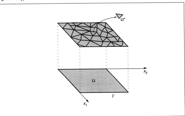
Since any polygonal structure with rectilinear or curved sizes can be expressed as a sum of triangular and quadrilateral elements, these form the basis for (unstructured) finite element meshes (Figure 3.1). For a real world application, a domain will typically be divided into hundreds, thousands, or hundreds of thousands of elements.

Figure 3.1 Typical Finite Element Mesh

For each element, a certain number of points or nodes are defined, which can be positioned along the boundary or the interior of the element. These nodes are the locations where the numerical value of the field variable will be determined.

X

1

X2

(27)

27 General Methodology

3.1.2 Interpolating Functions

The second step in the finite element is to represent the variation of the quantity of interest within each element, and implicitly- via the nodal connectivities- throughout the domain. Here, the field variable q is approximated by linear combinations of known elemental interpolation functions N,' (x). If Oh (x) is an approximate representation of

4(x),

the finite element method states

m

0e(X) - 0(x) N(x)i (3.1)

i=1

where m is the number of nodes in the element and qi are the nodal values. In general, the interpolation functions are simple polynomials that vanish outside the considered element. The components Oi are the unknown nodal values of the dependent variable

k.

The elemental shape functions are summed to give global interpolation functions N, (x), so that globally 0 can be expressed as

M

O(X) , qh(X) = Ni(x) i (3.2) 2=1

where M is the total number of nodes in the mesh. The global shape function Ni is obtained by assembling the contributions Ne of all elements to which node i belongs.

3.1.3 Equation Discretization

The most essential and particular step of the finite element approximation is to represent the equation as a discrete system of equations. To this end, one requires an integral formulation of the field equations to be solved. The method of weighted residuals is one general technique by which this can be achieved. Other possible integral formulations, based on a variational

(28)

28 , General Methodology

For purposes of illustration, consider a domain Q with closed boundary F where one seeks a solution to the problem

LO = g (3.3)

In the discrete case, the same problem can be stated as

Lh = g (3.4)

In general, qh does not satisfy the continuous equation, and a residual can be defined as

Rh = Lh - g 0 (3.5)

The method of weighted residuals requires the use of a set of trial functions O and a set of weighting functions W. The trial interpolation functions are n-th order polynomials which interpolate the field variable 0 within each element

h = { 9 o 4 , E pn(Qe)} (3.6)

The weighting functions are conceptually similar:

Wh = {Whe I We C pn(Qe)} (3.7)

The statement of the finite element approximation is as follows: find Oh E cph such that for all

Wh E Wh, so that the following variational statement is satisfied:

I

Wh Lh dQ = Wh g d (3.8) This can also be expressed more concisely as

f Wh Rhd = 0 (3.9)

If the weighting and trial functions differ, the method is known as the Petrov-Galerkin approach, otherwise the method is known as the Bubnov-Galerkin approach. The latter approach will be used for the remainder of this thesis.

(29)

29 Finite Element Library

The above integrals are computed for each weighting function Wh and the results are summed to give a system of discrete equations in the field variable q. A number of methods exist for solving such linear systems [5, 18]. Once the system has been solved, Eq. (3.2) can be used to find the approximate value of a quantity q anywhere in the domain.

An important property of the approach is that the discrete equations are always consistent. Note that the Galerkin approach states nothing about the stability of the resulting scheme. In the next chapter, the Galerkin method will be used to discretizate the Euler equations and boundary conditions, with due considerations given to efficiency and stability.

3.2 Finite Element Library

The choice of interpolation or shape functions determines the order of approximation for the discrete equations, which in turn affects the convergence rate. For future reference, the one-and two-dimensional linear elements are briefly described below.

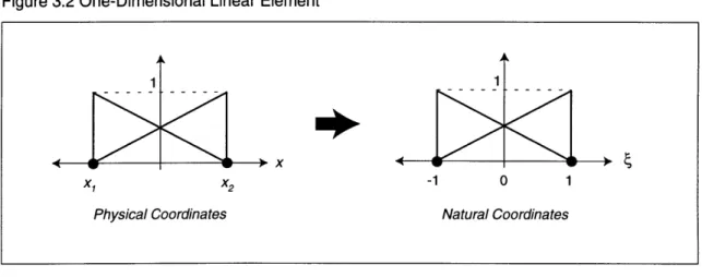
3.2.1 One-Dimensional Linear Elements

The simplest element consists of two nodes interpolated in a piecewise linear manner

(Figure 3.3). As such, the shape functions are discontinuous in slope at element boundaries. If one defines the local coordinate ( within each element through the mapping

X -= (3.10)

2Ax

the interpolation functions take the universal form

N( ₂ 1 2

₂

(3.11)

N = 1() 2 (3.12)

The Jacobian is the transformation matrix between the coordinate systems

IJI = = 2Ax (3.13)

(30)

Figure 3.2 One-Dimensional Linear Element

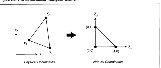
3.2.2 Two-Dimensional Triangular Elements

The two-dimensional linear triangular element consists of three nodes (Figure 3.4). Once again, the shape functions are discontinuous in slope at element boundaries. This is a particularly useful element type for fluid flow applications, as it is conceptually simple and useful in the discretization of complex geometries. The natural coordinate system employs barycentric coordinates with the mapping

1 = (al + blx + CLX ₂)

2A

1 -2

= _2where_A_is_{the area of the element and}(a2 + b2X1 + c2x2)

where

A

is the area of the element and

bt = x2,+1 - X_{2 f+2} CZ X1,+2 - Xl+1

(3.14)

(3.15)

(3.16)

The interpolation functions are

Nf() = ~1

N2 (C) = 6

N3(() = 1 - (1 - 5

The Jacobian matrix transforms between physical and elemental coordinates

IJI = 2A

(3.17) (3.18)

(3.19)

(3.20) This is simply twice the elemental area.

(31)

31 Finite Element Library

Figure 3.3 Two-Dimensional Triangular Element

(0,1)

X2

x

3

X x, x (0,0) (1,0)

Physical Coordinates Natural Coordinates

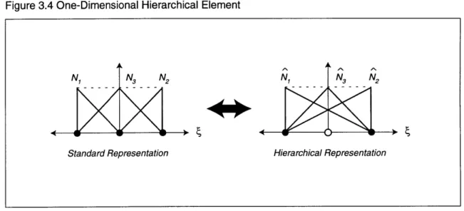
3.2.3 One-Dimensional Hierarchical Elements

Thusfar, only elements having a nodal basis have been considered. That is, the nodal value qi is exactly the value of the solution at the nodal location xi. There is another family of shape functions which satisfy the Raleigh-Ritz interpretation, but not a pointwise nodal one. The utility of such an element will become apparent in mesh adaption (§5.3.2). Essentially,

enriching the solution will be performed by adding new shape functions to the existing ones in such a way that enriching M nodes to M + 1 nodes will not change the existing shape functions and degrees of freedom, but only add new ones. This contrasts with traditional Lagrangian elements, where adding the M + 1 node requires redefining shape functions. These new interpolation functions are known as hierarchical shape functions.

Using hierarchical shape functions, one obtains an approximation of the unknown solution in the same form as usual

m

0e(x) ' ~e(x) = N(x)¢i ( (3.21)

i= 1

However, the degrees of freedom corresponding to the hierarchical shape functions cannot be interpreted as values of the solution at some node inside the element. Instead, they should be thought of as perturbations on top of the local solution value.

(32)

Figure 3.4 One-Dimensional Hierarchical Element

N, N N2 N N3 N2

Standard Representation Hierarchical Representation

The one-dimensional hierarchical element is formed if one enriches the linear element by placing an additional node at the midpoint of the element, with the further condition that the additional shape function vanish at the element boundaries (Figure 3.5). Such an element

spans the same function space as that obtained by dividing the original element into two, and applying standard linear shape functions to each half. This fact leads to the transformation matrix between the two representations

Ne = TNe = 1 N (3.22)

N e

With this relation, the interpolation functions can be written explicitly as

Nj() = (3.23) 2 1N() = 2 (3.24) 1+ for <0 N e(() = (3.25) 1- for >0

The element equations are now augmented to model the hierarchical node as:

TATT T-To = TF (3.26)

(33)

The values of the field variable are then computed as

O

= T4 = 1 2 (3.27)

The hierarchical node acts like a perturbation on the existing solution.

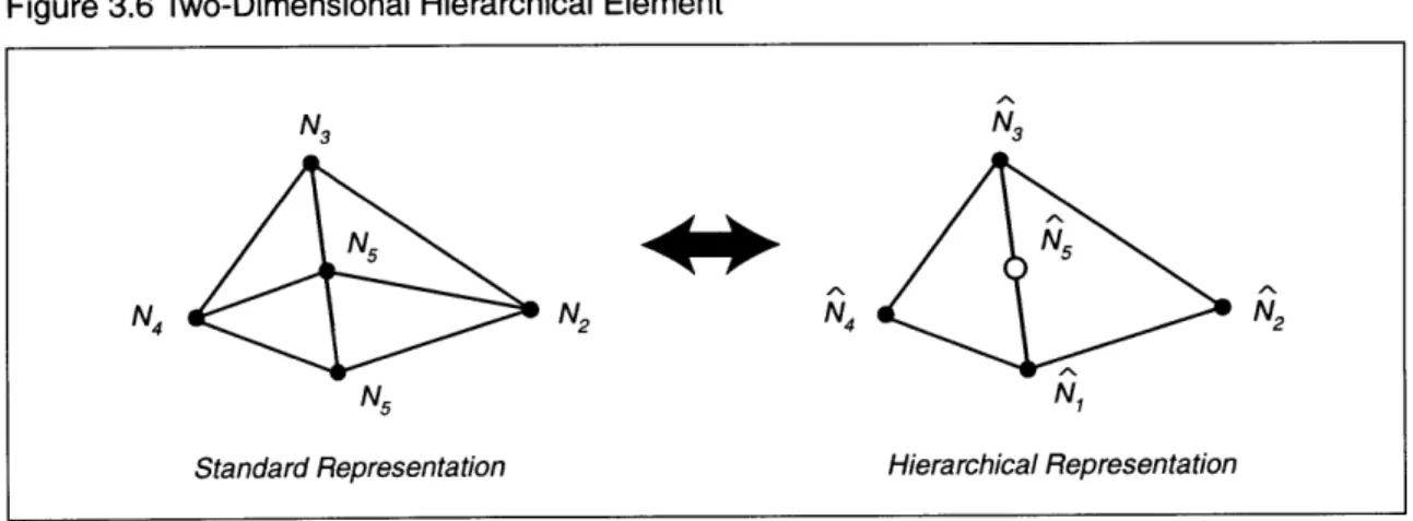
3.2.4 Two-Dimensional Hierarchical Elements

Two-dimensional hierarchical elements are essentially analogous to their one-dimensional counterparts, with the exception of the location of the hierarchical node. One can place the additional degree of freedom at the barycenter of the triangle or along an edge of the element (Figure 3.6). The latter is the preferred choice, as mesh refinement will be carried out by splitting edges rather than elements (§5.4.4). Splitting along edges also leads to anisotropic refinement, which lessens the computational cost of adaptive finite element solutions. By placing the the hierarchical node on an edge, the two neighboring standard elements each have an additional degree of freedom. The effect of hierarchical node can be removed from the global system through the process of static condensation, as its stencil is contained within the element patch. The value of the field variable at the additional degree of freedom can be computed by solving a local problem once the values of the surrounding nodes are known.

Figure 3.5 Possible Two-Dimensional Hierarchical Element Configurations

Hierarchical Node at Centroid

(34)

34 1 Finite Element Library

Figure 3.6 Two-Dimensional Hierarchical Element

N₃ N3

N5 N5

N4 N2 N4 N

N5 N1

Standard Representation Hierarchical Representation

The two-dimensional hierarchical element is equivalent to dividing the two adjacent elements into four (Figure 3.7). The transformation matrix between the two sets of interpolation

functions are 1000 N 0 1 0 0 0 N2 Ne TNe 0 0 1 0 N (3.28) 0 0 0 1 0 N4 0 0 0 0 1 \N5

The element equations are now augmented to model the hierarchical node as

TATT T-T = TF (3.29)

The values of the field variable are then computed as 1 0 0 0 0 1

0 1 0 00 02

=TT5= 0 0 1 0 0

/3

(3.30)

0 0 0 1 0 1 4

n 1 )0 4

(35)

4 Finite Element Algorithms

There exists a number of different schemes for solving the compressible Euler equations [7, 11, 20, 24]. In the present research, the steady two-dimensional Euler equations are solved using an implicit Newton scheme.

4.1 Galerkin Discretization

The Galerkin approach, as aforementioned (§3.1.3), uses the same trial and weighting function space to discretize the governing differential equation. As it stands, applying the Galerkin approach directly to the Euler equations does not work, as the resulting scheme lacks stability. This is due to the fact that the standard Galerkin finite element method gives rise to central difference-type schemes, which are unstable for convection-dominated problems.

The stabilized Galerkin finite element method enhances the stability of the standard Galerkin

finite element method through the addition of appropriate terms to the variational statement, which for scalar convection problems, corresponds to adding diffusion in the streamline

direction. In a sense, the stabilized Galerkin method is the natural finite element analogue to upstream-type finite difference or finite volume schemes.

It is also known that the resulting scheme may result in oscillatory behavior close to

discontinuities. To reduce these problems, a discontinuity-capturing term, which can be seen to add diffusion in the direction of the oscillations, must be added to the scheme.

(36)

36 Galerkin Discretization

4.1.1 Quasi-Linearized Form

In order to represent the Euler equations numerically, it is necessary to first write them in a

quasi-linear form. The quasi-linearized form of Eq. (2.1) is given by

V

A, = 0

where A, = - are the Jacobian matrices of the flux vector Fi given by

(4.1)

0 1

-

3u2±--1 u2

(3

-

)ul

-UlU2 U2

-yuie + (_ - 1)ullu|2

_e-

_-1 ₂

₊

_3U2)

0 -U1U2 A2 = S- 12 2 -yuze + (y - 1)u₂

u1

2 0 U2 -( - 1)ul - 1)UlU2 0 -(- 1)u 2 U₁ - (Y - 1)U1U2 1 U₁ (3 - 7)U2

ye- (u2

+

3u)

Note that the Ai matrices are not symmetric.

4.1.2 Finite Element Space

To obtain finite element approximations of the steady, two-dimensional Euler equations, consider a partition of Q into elements of triangles, with no overlapping amongst elements of the partition. The simplest conforming Galerkin method searches a solution Vh E Vh where

Vh = {V I V C pl (Qe)} (4.4)

The weighting functions are conceptually similar

Wh = {We I We E pl(pe)} (4.5)

The trial functions satisfy essential boundary conditions and the weighting functions are homogenous at these points.

(4.2) 0

0 -

i

YU2 (4.3)

(37)

The trial solution can be represented more explicitly as

M

Vh(x) = Ni(x)Vh, (4.6)

i= 1

where M is the number of nodes in the finite element mesh. The weighting functions satisfy

M

Wh(x) = Ni(x)Wh, (4.7)

i= 1

where Wh, are the nodal values of the weighting functions.

4.1.3 Weighted Residual Statement

The statement of the finite element weighted residual formulation is as follows: within each element pe, e = 1,..., E, find Vh E Vh such that for allWh E Wh, the following variational

equation is satisfied:

WE EVh Oh

OWh AiVh df e + A " - TAix d

axi

e e= _(4.8)

+ VVWh -VVh dQ =

J

-W -AiVh ni dF

e=1 Qe _r

The first and last integrals in Eq. (4.8) constitute the standard Galerkin formulation. The second integral is the stabilization term. Discontinuity-capturing properties are provided by the third term.

4.1.4 Weak Form

The first and last integrals in Eq. (4.8) constitute the weak form of Eq. (4.1), obtained by integration-by-parts:

Wh

-

A i dQe = 0

xzi

-- - AiVh d e + Wh -AiVh ni dF = 0(4.9)

t e r

(38)

The weak form of the Euler equations is preferred for several reasons. Firstly, the integration-by-parts form gives rise to natural boundary conditions without modification to the scheme. The weak form is also necessary for allowing discontinuous solutions, which arise due to shocks. Such discontinuous solutions do not satisfy Eq. (2.1) in the classical sense, as they are not differentiable. The Rankine-Hugoniot equations relate the jump in the solution variable to the speed of propagation of the discontinuity. Unfortunately, solutions of the weak form are not unique and the (physically) correct one must satisfy the full viscid equations in the limit of vanishing viscosity. Such a solution is called entropy-satisfying.

4.1.5 Stabilization

The scheme proposed in Eq. (4.9) by itself is unstable. To observe this, consider the one-dimensional pure convection limit of Eq. (2.1):

dVh V + A AVhV = 0 _(4.10)

with A constant. The element equations for a typical interior node are given by

S NNe d a- -

J

N- AVh, dfe (4.11)

i=1 e e

It is apparent that the equation is satisfied by a sawtooth mode, with alternative values at successive nodes. The implication of this observation is that the numerical scheme needs to spatially stabilized to ensure the elimination of such modes [5].

One method of stabilizing the standard Galerkin approach is through the addition of a small diffusion-like term to Eq. (4.8). For the current scheme, this term can be represented as

E _Wh

AVh

A O- A d e (4.12)

e=1 Qe

and

7

is a positive scalar which has the dimensions of time and a magnitude which is of the order of the mesh spacing h. The stabilization term can be seen to add diffusion in the streamline upwind direction, in a manner analogous to the finite difference and finite volume counterparts.

(39)

To ensure consistency, the term is made proportional to the residual. It can be readily

demonstrated that this modification to the Galerkin statement results in a stabilized numerical scheme. In the present scheme, -r is taken to be:

h 1

h

=

(4.13) 2 ul + a

Other authors [6, 11] have proposed alternative definitions for r.

4.1.6 Discontinuity-Capturing

The third integral in Eq. (4.8) is the discontinuity-capturing operator, required for controlling

overshoots and undershoots near discontinuities. To stabilize the solution, one uses the fact that an approximate solution Vh exists everywhere in the domain. This solution does not necessary fulfill the differential equation:

Rh = LVh 5 0 (4.14)

where L A, - is the differential operator. The size of the residual IRhl will be small away from discontinuities and large close to a shock. This qualifies Rh as a base for constructing an automatic artificial viscosity which adds O(h) smoothing close to the discontinuity and vanishes in smooth regions. It can be seen that this term adds diffusion in the direction of the gradient.

The discontinuity-capturing factor v is a scalar taken to be

v = h (4.15)

IVV I

Note that the definition of v is proportional to the residual LVh. The gradient of Vh is included to normalize the artificial viscosity. To avoid confusing dimensions, the Vh occurring Eq. (4.15) should be made nondimensional.

(40)

40 i Numerical Implementation

4.2 Numerical Implementation

The weighted-residual statement in Eq. (4.8) can now be written explicitly as a system of algebraic equations for subsequent implementation on computer. Substituting Eqs. (4.6- 4.7) into the Galerkin/least-squares variational equation leads to:

M E I M L M E M

wh{

h

VNa . VNbVb de + La TZ

LbVb

a=1 e=e h =1 VNdVhd b=1 e=1Qe b=1

- NaA (ANbVhb dnQ + NaAi ( NbVhb) ni d = 0 (4.1

Ge b=1 (b=1

where L is again the differential operator. Define the solution vector as

e6)

16)

(4.17) V= {vT, V ,..., T V

Then Eq. (4.16) can be written as

Wh -Rh = 0 (4.18)

where Rh is an (4 M) x 1 system of nonlinear algebraic equations with Vh as its vector of nodal unknowns. For nodes located in the interior of the computational domain, Eq. (4.16) leads to the nonlinear algebraic system

Rh = 0 (4.19)

The above algebraic system is implemented on the computer employing an element-based data structure, with each element represented by a sequence of edges and nodes. This particular hierarchy was developed with both flexibility and modularity in mind and it lends itself to efficient implementation of adaptive meshing procedures. Further details concerning the coding structure can be found in Appendix C.

The integrals in Eq. (4.16) are approximated using Gaussian integration:

P

f(x) d e wp f (EP) J

Qe p=l

where P refers to the number of integration points in the element and wp are the Gauss integration weights [25]. Single point quadrature is assumed hencetoforth.

(41)

41 Numerical Implementation

4.2.1 Solution Techniques

A Newton iterative solution procedure is used to solve the nonlinear algebraic system, Eq. (4.19). Let V n") be the n-th iterative approximation for Vt( ), the desired steady-state prediction. The Taylor series expansion of R, retaining only the first two terms, yields

R(V(

R(V R(V()) AV (n) = 0 (4.21)

aV

where

AV (n) E V(n+I) - V (n) (4.22)

Newton methods offers second-order convergence rates but requires formation of the Jacobian matrix -. In the present research, a Newton method is used because the Jacobian matrix is further required for mesh adaption procedures.

Denote the residual vector and consistent tangent matrix by

R"() = R(V(n)) (4.23)

M(n) =R(V(")) (4.24)

av

Then R(") can be written for a given node a as

R(n) = - aONa NbVb de NbV dQ x (b=1 be b=1( ne (4.25) +f ( A A -X Vb) dfe + fNaA NbVb=l ni dr

(

M e b=1 b=1 where v is given by JIj Em, Nb Vb S=h bAi =1 a b (4.26)

where 6 is a small number to avoid division by zero. The consistent tangent matrix M(n) is computed by differentiating the residual vector by the state vector.

(42)

42 Numerical Implementation

Differentiating Eq. (4.25) gives:

M(n ) - AiNb dQ e" - D MaEAi NcV, dNc e

ab e _c=1

f

ONbI INa dQe + v Na Vc dQ

DXi

Dxi Vb Dxi 1ix

rr c=1 M

(

M

+

Na

A ,7-('M c + AJ

ANb

ddNe

±

xiAV .±T 0

(DNaAi)

A Aj M DN d

+

-xi

E xj

i

e / DVne i c=1

The solution of the nonlinear system is computed by solving

(4.27)

(4.28) M(n)AV(n ) = -R (")

V(n"1) = V(n) + AV ( n )

at each iteration. An incomplete linear LU preconditioned GMRES solver is used to solve for AV at each iteration. Appendix C provides further details concerning the implementation of the solver. Figure 4.1 summarizes the algorithm used to solve the system.

Figure 4.1 Implicit Solution Algorithm for the Euler Equations

Write final solution Read restart solution Assemble system matrices Newton solution algorithm Update solution vector Check termination clause

(43)

43 Numerical Implementation

4.2.2 Wall Boundary Conditions

At a solid surface boundary, there is no mass flux normal to the boundary. This constraint can be expressed in a coordinate system aligned with the solid surface:

P P

S un 10 (4.29)

put put

pe / pe

This can also be represented in terms of the change AV as

Ap

(I

A

AV = = (4.30)

Aput Aput

Ape Ape

The assembled global system equation corresponding to a given boundary node is

L. . Mab ... J AVa = -Ra (4.31)

For the purposes of implementation, the transformation matrix between Cartesian and body-fitted coordinates is defined as

1 0 0 0

, 0 n,, ny O 0 _(4.32)

0 -nY n 0

0 0 0 1/

Applying the transformation to nodal equation Eq. (4.31) gives

L[ TMabT-' --J AVa = -TRa (4.33)

The wall boundary condition is imposed by zeroing out the row corresponding to the momentum normal to the surface and placing a one on the diagonal. The resulting equations are transformed back to Cartesian coordinates and replace those in the global system.

(44)

44 Numerical Implementation

Table 4.1 Imposed Variables at Exterior Boundaries

Boundary Ap Aul Au2 Ap As Ah

Subsonic Inlet - u, -ul u2, -U2 - Si - 800 hi - hoo

Supersonic Inlet - Free U2, -22, - Si - sC hi - hoo

Subsonic Outlet Free Free Free pi - poo

Supersonic Outlet Free Free Free Free

4.2.3 Exterior Boundary Conditions

At the farfield, different boundary conditions are imposed based on the direction of the characteristics and the local Mach number (§2.2.2). In the current scheme, the state vector V = (s, u1, u2, h) is used to prescribe values at inlet and V = (p, ul, u2, p) at the outlet.

Table 4.1 summarizes which set of variables is to be used under the various conditions. Prescribed quantities are imposed in a manner similar to that described for wall boundary conditions. The transformation matrix between the AV and AV state vectors is

('y- 1)((y+I) uI-2 ,ye) (-y-l)ul

2p' pY' RL 1 P p p -y _ (--1)U

SP

P P p--Y p- p1 0 0 1 ₀ S(Y--1)u2 y P P

The corresponding transformation matrix between AV and AV is given by

1 T= P P 2 0 1 p - 1)U -(y - 1)u2

0

0 0

(4.35)

Note that imposing boundary conditions using the penalty approach will not work in this case, due to dimensional considerations.

(45)

45 Test Cases

Table 4.2 Cosine Bump Test Parameters

Quantity Symbol Case 1 Case 2 Case 3

Mach Ma 0.5 0.675 1.75

Nodes M 5048 6383 8483

Elements E 9800 12457 16631

Iterations n 10 26 42

4.3 Test Cases

Several test cases, comprising both internal and external flows under subsonic, transonic, and supersonic conditions, were run with the implemented Euler flow solver in order to gauge performance and accuracy. The cases were conducted using relatively fine computational meshes, and as such, they represent the order of accuracy desired for solutions obtained after using adaptive techniques.

4.3.1 Cosine Bump

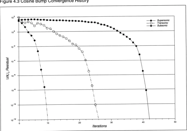
The computational domain consists of a rectangular channel with dimensions of 3 x 1 units, on the bottom surface of which a 10% high cosine bump is located (Figure 4.2). The upper and lower surfaces are walls, and the flow proceeds from left to right. Tests were conducted at Mach 0.5, 0.675, and 1.75. Table 4.2 summarizes grid and flow quantities for the simulations.

Results show that convergence rates for all three cases were initially slow, but approached the expected second-order behavior after several iterations (Figure 4.3). Convergence in the initial iterations was possibly limited by strong underrelaxation. All simulations were converged to the 1.0 x 10-12 in the residual norm. Figures 4.4 to 4.6 show the computational mesh, pressure and Mach contours for each test case. Both the transonic and supersonic grids were refined in the vicinity of shocks in order to capture the discontinuities more exactly. Overall, the results seem to validate the accuracy and efficiency of the solver.

(46)

46 Test Cases

Figure 4.2 Cosine Bump Geometry

Figure 4.3 Cosine Bump Convergence History

Iterations

(47)

47 Test Cases

Figure 4.4 Cosine Bump Results at Mach 0.5

1.00 Initial Grid 0.90 0.80 0.70 0.60 0.50 0.40 0.30 0.20 0.10 0.00 -1.00 -0.50 0.00 2.254 2.307 2.359 2.412 2.464 2.517 2.569 2.622 2.674 2.726 2.779 2.831 2.884 2.936 2.989 -1.00 -0.50 0.00 0.426 0.451 0.477 0.502 0.528 0.554 0.579 0.605 0.630 0.656 0.682 0.707 0.733 0.758 0.784 0.50 0.50 1.00 1.50 2.00 ~ ~BS~B~f~C~G/89~E

(48)

48 Test Cases

Initial Grid -0.50 0.00 0.566 0.648 0.730 0.812 0.894 0.976 1.057 1.139 1.221 1.303 1.385 1.467 1.549 0.00 0.50 047 050 059 .2 .66 065 079 .1 .8 099 102 1.0 .7 .21 134 139 .7 .4 2.00 I : ==w==M.& 1.630 1.656 1.712 0.447 0.520 0.593 0.620 0.666 0.695 0.739 0.812 0.885 0.959 1.032 1.105 1.178 1.251 1.324 1.397 1.470 1.543

(49)

-0.50 0.00 0.50 1.00 1.50 2.00 -0.50 0.00 0.50 1.00 1.50 0.121 0.157 0.192 0.228 0.263 0.299 0.334 0.370 0.405 0.441 0.476 0.512 0.547 0.583 0.619 0.654 0.690 0.725 -0.50 0.00 0.50 1.00 1.50 0.788 0.877 0.966 1.055 1.143 1.232 1.321 1.410 1.499 1.588 1.677 1.766 1.855 1.944 2.033 2.121 2.210 2.299 49 Test Cases

-1.00

-1.00 2.00

(50)

50 1 Test Cases

Table 4.3 Symmetric Airfoil Test Parameters

Quantity Symbol Case 1 Case 2 Case 3

Mach Ma 0.5 0.8 1.75 Angle a 40 20 00 Nodes M 7758 8193 8255 Elements E 15310 16174 16304 Iterations n 38 64 56

4.3.2 Symmetric Airfoil

The computational domain consists of a circle of radius 10 units, with the leading edge of the unity chord length symmetric NACA 0012 airfoil located at its center (Figure 4.7). Test cases were run at Mach 0.5 at a = 40, 0.8 at a = 20, and 1.75 at a = 00. Table 4.3 summarizes parameters used in the tests.

Convergence rates for all three cases exhibit similar trends as those observed in the cosine bump test cases (Figure 4.8). All simulations were converged to within 1.0 x 10-12 in the

residual norm. Note that no special boundary corrections were applied at the farfield boundary.

Figures 4.9 to 4.11 show the computational mesh, pressure and Mach contours for each test case. Both the transonic and supersonic grids were refined in the regions near shocks. In general, the results seem reasonable and appear to be properly resolved.

(51)

51 Test Cases

Figure 4.7 Symmetric Airfoil Geometry

Figure 4.8 Symmetric Airfoil Convergence History

Iterations

10

- 2

104

(52)

52 i Test Cases

Figure 4.9 Symmetric Airfoil Results at Mach 0.5

1.50 I nitil ril 1.00 0.50 0.00 - -0.50--1.000 -1.50 -1.50 -1,00 -0.50 0.00 0.50 1.00 1.50 2.00 2.50 1.501.00 -0.00 0.50 --1.00 --1 .5 0 f 1 , I I i I ,I I I I I I I I I I I I I I I I I -1.50 -1.00 -0.50 0.00 0.50 1.00 1.50 2.00 2.50 1.50 . 1.00- 0.50- 0.00- -0.50- -1.00--1,.50 -1.00 -0.50 0.00 0.50 1.00 1.0 2.00 2.5 -1.50 -1.00 -0,50 0.00 0.50 1.00 1.50 2.00 2.50 Pressure Contours

. ..

...

_/

..

_.

_\

t~

~ ~ ~

...

~.

...

.

...

.

-- --- / '" "' .\ Mach Contours I 0.870.83 0.79 0.75 0.71 0.67 0.64 0.60 0.56 0.54 0.53 0.48 0.48 0.47 0.44 0.40 0.37 0.33 0.29 0.25 0.21 0.17 0.14 0.10 0.06

(53)

53 Test Cases

1.50 Initial Grid 1.00 0.50 0.00 0.50 1.00 --1.50 -1.50 -1.00 -0.50 0.00 0.50 1.00 1.50 2.00 2.50 1.50 Pressure Contours 1.48 1.36 1.31 1.00 / 1.25 1.17 1.1 5 1.11 0.50 1.08 0.96 0.91 \ / / -\ 085 -0.50\ _i 1.00 - -1.50-0.00 _1.50. 1.00 0.50 0.00 0.50 1.00 1.0 2.00 2.0 Contours , 1.34 -0.50 / _I_\-0.26 0.32 S-1.22 1.000.13 1.0-1.00 -1.00--1.50

(54)

54 Test Cases

1.50 Initial Grid 1.00 -0.50 -0.00 -0.50 - -1.00--1.50 -1.50 -1.00 -0.50 0.00 0.50 1.00 1.50 2.00 2.50 1.50 -Pressure Contours 0.82 0.74 0.70 0.66 1.00 -0.62 0.57 0.53 0.49 0.45 0.50 -0.41 0.37 0.33 0.28 0.24 0.22 0.00 0.20 0.18 -0.50 -1.00 -1.50 -1.50 -1.00 -0.50 0.00 0.50 1.00 1.50 2.00 2.50 1.50 1.9 Mach Contours /.86 1.83 1.76 1.67 .00 1.55 1 34 1.24 1.14 0.50 - 1.03 0.83 0.72 0.62 0.52 0.00.. 0.41 0.31 0.21 0.10 1.00 --1.50 1- . .... -1.50 -1.00 -0.50 0.00 0.50 1.00 1.50 2.00 250

(55)

5 Mesh Adaption Fundamentals

Adaption is the process by which some aspect of the solution algorithm changes in response to an evolving solution. These changes can be in the discrete equations, in the computational mesh, or in both the equations and the mesh. In the present work, adaption refers to changes in the computational mesh as the solution proceeds.

5.1 Requirements of the Adaption Procedure

In a typical problem, one starts out with an idea of what the flow will look like, but one usually does not know exactly where the interesting flow features (shocks, boundary layers, and recirculation zones) lie. The adaptive approach starts with an initial mesh, coarse enough to be inexpensive to compute, yet fine enough so that most of the essential features can appear. The first step in the adaptive solution procedure is to compute the solution on this initial coarse mesh. Then, certain elements are flagged for refinement, based on some local error estimates. Elements are divided, the solution is interpolated on the new grid, and the calculation proceeds anew until the solution is sufficiently resolved (Figure 5.1).

Figure 5.1 Mesh Adaption Algorithm

Write final solution Read restart solution

Assemble and compute solution Flag elements for refinement Alter computational mesh Update solution vector

(56)

56 1 Optimal Mesh Criteria

Any grid adaptive procedure is comprised of three main ingredients:

1. Optimal mesh criteria. Used to determine whether the computational mesh is sufficiently fine to properly resolve the flow.

2. Error indicators. Highlights, through some local error estimation techniques, regions where mesh refinement/derefinement is beneficial.

3. Refinement procedures. An actual algorithm for the addition, subtraction, or redistribution of nodes in the mesh.

Each of the above components will now be analyzed in detail, with particular emphasis on the methodologies used in the current implementation.

5.2 Optimal Mesh Criteria

Before designing an adaptive mesh procedure, one should have a clear idea of what is to be achieved. Although an obvious answer is the reduction of manual and computational work, a more quantitative assessment of the optimality of the adaptive mesh procedure is desirable. What should the optimal mesh be like? An answer to this question is seldom clear, as one

does not know a priori what constitutes a sufficiently accurate answer to the problem at hand.

Many researchers [12, 13] consider an solution acceptable if the estimated error satisfies some prescribed global or local conditions. This definition of an optimal mesh leads to a stopping

criteria, which controls whether mesh adaption is necessary in order to satisfy the optimality

(57)

57 1 Optimal Mesh Criteria

5.2.1 Equidistribution of Error

A very popular criterion is that a mesh is considered optimal if the distribution of the error is equal amongst all the elements in the mesh. Conceptually, one can derive this criterion from the observation that the error will have the irregular distribution for the first mesh shown in Figure 5.2. If the number of degrees of freedom is kept the same, the distribution of element size is all that can be varied. After a repositioning of nodes, the error distribution in space becomes more regular.

In many applications, the required error I 1 on a given mesh may not be the same at all locations. The equidistribution of error concept, applied locally, can lead to even more cost-effective grids. That is, instead of using the general minimization

min Ihl - EIjl over entire domain (5.1)

one may desire to only consider certain regions of the domain

min

lhl

- J1e| over subdomain (5.2)

where |Eh| represents the local error level. Mesh refinement would then take place if the local error indicator exceeds or falls below specified refinement or coarsening tolerances.

Figure 5.2 Error Distribution Before and After Refinement

Before Refinement

I I I I IIll I I I I

I I I I I I I I I I I I I I I

Adaptive finite element solutions of the steady Euler equations using a sensitivity approach