HAL Id: hal-03013331
https://hal.archives-ouvertes.fr/hal-03013331
Submitted on 18 Nov 2020HAL is a multi-disciplinary open access archive for the deposit and dissemination of sci-entific research documents, whether they are pub-lished or not. The documents may come from teaching and research institutions in France or abroad, or from public or private research centers.
L’archive ouverte pluridisciplinaire HAL, est destinée au dépôt et à la diffusion de documents scientifiques de niveau recherche, publiés ou non, émanant des établissements d’enseignement et de recherche français ou étrangers, des laboratoires publics ou privés.
The value of coarse species range maps to inform local
biodiversity conservation in a global context
Isabelle Maréchaux, Ana S.L. Rodrigues, Anne Charpentier
To cite this version:
Isabelle Maréchaux, Ana S.L. Rodrigues, Anne Charpentier. The value of coarse species range maps to inform local biodiversity conservation in a global context. Ecography, 2016, 40 (10), pp.1166 - 1176. �10.1111/ecog.02598�. �hal-03013331�
practice, though, range maps are generally coarse representa-tions of species’ global distribution, often closer to species’ ‘extent of occurrence’ (broad envelopes encompassing their known occurrences), than of ‘area of occupancy’ (where the species is truly present; Gaston and Fuller 2009). When compared with occupancy data from field sightings (Graham and Hijmans 2006, Hurlbert and Jetz 2007, Cantú-Salazar and Gaston 2013), range maps suffer particularly from commission errors (when a species is considered present in a site from where it is absent) but also from omission errors (when a species is considered absent in a site where it occurs; Rodrigues et al. 2004b, Rondinini et al. 2006). Comparing bird range maps with fine-scale (∼ 0.25° resolution) data from atlases in Australia and South Africa, Hurlbert and Jetz (2007) found commission errors to be scale-dependent: species were absent on average from 47 and 36% (respec-tively) of the grid cells overlapping their range maps, but from only 2 and 5% of coarser 2° cells, and from nearly none 4° cells. Based on these results, Hurlbert and Jetz (2007) recommended that range maps should only be used to infer species presence at spatial resolutions of 1° (about 12 400 km2 at the Equator), or even coarser for taxa not as
Ecography 40: 1166–1176, 2017
doi: 10.1111/ecog.02598 © 2016 The Authors. Ecography © 2016 Nordic Society Oikos Subject Editor: Jeremy T. Kerr. Editor-in-Chief: Miguel Araújo. Accepted 23 August 2016
In 2004, the International Union for Conservation of Nature (IUCN) completed the first evaluation of the conservation status of all amphibian species as part of the IUCN Red List of Threatened Species, accompanied by the release of nearly 6000 range maps (Stuart et al. 2004). Since then, the IUCN has made freely available for non-commercial use range maps for about 50 000 species, includ-ing all mammals, all birds, thousands of marine species (e.g. fishes, sea snakes, corals, lobsters, seagrasses) and thousands more of freshwater species (e.g. fishes, crustaceans, molluscs, odonatans, turtles, plants) (available from IUCN 2014). Thousands of other species, covering an expanding diversity of taxa, are under assessment.
These species range maps are increasingly being used in spatial conservation planning exercises (Rodrigues et al. 2004b, Wilson et al. 2010, Pompa et al. 2011, Pouzols et al. 2014). For analytical purposes, the polygons represent-ing each species’ range are typically rasterised into a grid, resulting into a dataset of species’ presence/absence per site. Inputting these data into conservation planning analyses is done under the (explicit or implicit) assumption that spe-cies occur in all sites where mapped, and only in those. In
The value of coarse species range maps to inform local biodiversity
conservation in a global context
Isabelle Maréchaux, Ana S. L. Rodrigues and Anne Charpentier
I. Maréchaux ([email protected]), A. S. L. Rodrigues and A. Charpentier, CEFE UMR 5175, CNRS – Univ. de Montpellier – Univ. Paul-Valéry Montpellier – EPHE – CNRS, Montpellier, France. IM also at: AgroParisTech ENGREF, Paris, France. Present address of IM: Laboratoire Evolution et Diversité Biologique, UMR 5174 CNRS-UPS, Univ. Paul Sabatier, Toulouse, France.
Range maps of thousands of species, compiled and made freely available by the International Union for Conservation of Nature, are being increasingly applied to support spatial conservation planning. However, their coarse nature makes them prone to commission and omission errors, and they lack information on the variations in abundance within species’ distributions, calling into question their value to inform decisions at the fine scales at which conservation often takes place. Here, we tested if species ranges can reliably be used to estimate the responsibility of sites for the global conservation of species. We defined ‘specific responsibility’ as the fraction of a species’ population within a given site, considering it useful for prioritising species within sites; and defined ‘overall responsibility’ as the sum of specific responsibility across species within a site, assuming it informative of priorities among sites. Taking advantage of an exceptionally detailed dataset on the distribution and abundance of bird species at a near-continental scale – a level of information rarely available to local decision-makers – we created a benchmark against which we tested estimates of responsibility derived from range maps. We investigated approaches for improving these estimates by complementing range maps with plausibly available local data. We found that despite their coarse nature, range maps provided good estimates of sites’ overall responsibility, but relatively poor estimates of specific responsibility. Estimates were improved by combining range maps with local species lists or local abundance data, easily available through local surveys on the sites of interest, or simulated expert knowledge. Our results suggest that combining range maps with local data is a promising route for improving the effectiveness of local conservation decisions at contributing to reducing global biodiversity losses. This is all the more urgent in hyper-diverse poorly-known regions where conservation-relevant decisions must proceed despite a paucity of biodiversity data.
well-known as birds, such as amphibians or insects. For com-parison, 75% of the world’s protected areas are smaller than 100 km2 (IUCN and UNEP-WCMC 2012).
Furthermore, given that range maps only represent the limit of species’ distributions, they contain no information on the variation in abundances across species’ ranges. Their application to conservation planning therefore also assumes (implicitly or explicitly) that all sites where a species occurs are equally important to the species’ conservation. Indeed, area targets commonly applied in conservation planning (i.e. that a given species should be represented in protected areas by at least X% of its range; Rodrigues et al. 2004b, Pompa et al. 2011, Pouzols et al. 2014), make sense under the assumption that the fraction of the species’ range is a good surrogate for the fraction of the total population protected. In practice, however, this is not necessarily true: abundance often varies substantially across species’ ranges, with most species being rare at most sites where present and abundant at relatively few (Gaston 2003). Information on the fraction of each spe-cies’ global population at a given site is used to identify sites of global importance for conservation, including Ramsar Wetlands of International Importance ( 1%; Convention on Wetlands 1971) and Alliance for Zero Extinction sites ( 95%; Ricketts et al. 2005). However, such information is seldom available to local conservation planners, as (other than for species with very small ranges or that aggregate con-spicuously, which can be censused relatively easily) obtaining it requires much human and monetary investment.
Given these limitations, the application of range maps to conservation planning may lead both to wasted invest-ments to protect species in places of little or no value to their conservation, and conversely to missed opportunities to invest strategically in high-value sites. In order to quan-tify these effects, we focus here on the percentage of each species’ population within a site as a measure of the site’s responsibility for the global conservation of the species. We consider both this measure of ‘specific responsibility’ (defined for each species in each site) and an aggregated measure of ‘overall responsibility’ (defined for each site, as the sum of the specific responsibility values for all species in the site). We evaluate the effectiveness of coarse range maps for inform-ing conservation decisions at the local scale by comparinform-ing estimates of specific and overall responsibility derived from IUCN range maps with a high quality benchmark obtained from an exceptionally detailed dataset on the distribution and abundance of bird species at a near-continental scale (Sauer et al. 2007). This allows us to go further than previous studies that analysed the effectiveness of range maps in rep-resenting species’ occupancy (Graham and Hijmans 2006, Hurlbert and Jetz 2007, Cantú-Salazar and Gaston 2013) by also evaluating the performance of range maps in represent-ing the abundance structure of real distributions.
Furthermore, we test practical approaches for improving responsibility estimates by complementing range maps with other data plausibly available to local managers. We start by testing an approach for overcoming the limitations of range maps in representing occupancy, and then test two approaches for also taking into account the abundance structure of species’ distributions. From these results, we derive practical recommendations for making the best use of available data to improve estimates of site responsibility
for the conservation of species, as a contribution to better inform local-scale decision-making within a global biodiver-sity conservation context.
Material and methods
All calculations and analyses were done in R (R Development Core Team), particularly the ‘maptools’ R package (Bivand and Lewin-Koh 2010). All maps were done in ArcGIS 10.1, using the North America Albers Equal Area Conic projection (ESRI 2012).
Species distribution data
We obtained from the IUCN Red List of threatened spe-cies spespe-cies range maps representing the global breeding distribution of 316 land birds in the United States and Canada (BirdLife International and NatureServe 2012). We considered only parts of the species’ range where they are classified as extant or probably extant, native or reintroduced, and where they occur as breeding migrants or as residents.
We obtained high-quality distribution and abundance data from the North American Breeding Bird Survey (BBS; Sauer et al. 2007) for the same 316 species. The BBS is a long-term (since 1966) annual avian monitoring program, in which volunteers count the numbers of birds observed along roadsides survey routes. There are currently 3700 active BBS routes, of which nearly 2900 are surveyed annu-ally, following a standardized protocol: each survey route is randomly located and 24.5 miles long, with a 3-min point count conducted at 0.5-mile intervals, during which every bird seen or heard within a 0.25-mile radius is recorded. In our analyses, we used a derived dataset consisting of a layer of estimated relative abundance per species across an orthogo-nal grid (cell size ∼ 462 km2; hereinafter referred to as ‘sites’, and corresponding to a ‘local scale’). This was obtained by combining the 2006–2010 raw annual count data, first by calculating the average number of individuals counted per route, and then by smoothing these average counts across sites, cutting values below a threshold of minimal relative abundance of 0.1. For many of sites, particularly in regions with sparser BBS coverage, abundance values are therefore estimates derived from count data in neighbouring areas. This averaging and smoothing likely reduce the noise created by natural spatial and temporal variabilities (e.g. reduc-ing the impact of records of vagrant individuals), makreduc-ing the BBS data more comparable to the IUCN range maps. The final relative abundance layer predicts for each site the average number of birds of the species that could be seen in about 2.5 h of birdwatching along roadsides, by very good birders (for details see Sauer et al. 2007).
Our study region covers the contiguous United States and southern Canada (up to latitude 55°N), corresponding to 23 608 sites (each with an area of ca 462 km2). For each site, we had therefore: species presence/absence derived from the IUCN range maps; and species’ relative abundances (and hence also their presence/absence) derived from the high-quality BBS dataset. The latter is not perfect – as in other data obtained from field surveys, it is biased towards some
species and habitats (Keller and Scallan 1999, Bibby et al. 2000) – but it is the best available fine-scale dataset on the distribution and abundance of a taxonomic group at a near-continental scale. For the purposes of these analyses, we treated it as if it perfectly represented species’ distributions.
Quantifying commission and omission errors
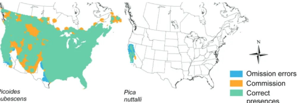
For each species, we calculated (Fig. 1): 1) percentage of commission errors: percentage of the total number of sites overlapping the range map from where the species is absent according to the BBS data. 2) Percentage of omission errors: number of sites not overlapping the species range map but where the species is present according to the BBS data, in relation to the total number of sites overlapping the species range.
We investigated the distribution of both types of errors across species through histograms splitting species into 10%-width classes of error. In addition we investigated how commission and omission errors related to species’ range sizes by analysing the Spearman rank-order correlation between the mid-interval error value and the median range size of the species in each class.
Calculating reference values of ‘specific responsibility’ and ‘overall responsibility’ for each site
We use the term ‘specific responsibility’ to refer to the per-centage of the population of a given species that is found at a given site. We consider this a measure of the extent to which the site affects the global conservation options for the species, while recognising that in real life this may not be a perfect measure (e.g. it may under or over-estimate site value because of source-sink population dynamics [Heinrichs et al. 2010]).
We calculate reference values of ‘specific responsibility’ from the BBS data. For species whose global range falls completely within the study region, this was calculated as:
species local abundance inthe site sumof species local abundance
’
’ aacross study region ×100
For any species whose range falls partially outside the study region, values were corrected by taking into account the fraction of the species’ global range outside the region:
species local abundance inthe site sumof species local abundance
’
’ aacross study region IUCN global range study region
IUCN glob
×
× ∩
100
aal range
where ‘IUCN global range ∩ study region’ represents the area of overlap between the species’ global range and the study region. This correction assumes that average abundance is similar inside and outside the study region (such that, for example, if the study region covers 50% of the range, it is assumed that it includes 50% of the global population). Failure to meet this assumption may affect the veracity of the calculations of specific responsibility for these spe-cies, which may thus underestimate or overestimate the real fraction of the species’ total population in each site. However, this is unlikely to affect the conclusions of this study, whose purpose is not to identify real-life conservation priorities in North-America, but to compare approaches for better estimating reference values of responsibility assumed as perfect.
For any given site, we then calculated ‘overall responsibil-ity’, as the sum of specific responsibility values for all the species present at the site.
Metrics for measuring the value of range maps to estimate site responsibility
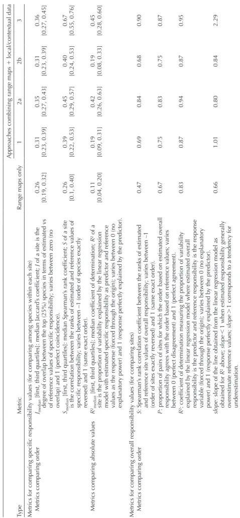
We estimated specific responsibility of each site for each species as the percentage of the species’ range overlapping the site. Overall responsibility was then estimated as the sum of specific responsibility values for all species whose ranges overlap the site. We evaluated the quality of these estimates by comparing them with reference values of responsibility, using a diversity of metrics (Table 1) that compare values either in terms of relative order (to investigate if estimates are good indicators of relative priorities) or in terms of abso-lute values (to understand if estimates can be used as direct measures of absolute responsibility).
Figure 1. Examples of the comparison between species range maps (from the IUCN data) and areas of occupancy (from the BBS data) for two of the bird species analyzed: correct presences are sites where the two types of distribution data match; commission errors are sites were the species is present according to the range maps but absent according to the BBS data; omission errors are sites were the species is absent according to the range maps but present according to the BBS data.
Table 1. Effecti veness of estimates of sites’ specific responsibility and of ov er all responsibility , obtained either from range maps alone, or by combining those maps with plausibly av ailable data through different approac hes: Approac h 1 (r ange maps local species lists); Approac h 2a (r ange maps local species lists continental expert kno wledge); Approac h 2b (r ange maps local species lists regional expert kno wledge); Approac h 3 (r ange maps local species lists local abundance data). Effecti veness w as assessed in eac h case through metrics that contr ast estimated values with the cor -responding reference v
alues, either in terms of order or in terms of absolute v
alues. F
or
Approac
hes 2 and 3, results are presented for respecti
vely m 8 and v 1. Approac hes combining r ange maps local/contextual data Type Metric
Range maps only
1
2a
2b
3
Metrics for comparing specific responsibility v
alues (for comparing among species within eac
h site)
Metrics comparing order
Jmedian
[first, third quartiles]: median J
accard’
s coefficient;
J of a site is the
degree of o
verlap between the top (25%) species in terms of estimated vs
of reference v
alues of specific responsibility; v
aries between zero (no
ov
erlap) and 1 (perfect coincidence).
0.26 [0.19, 0.32] 0.31 [0.23, 0.39] 0.35 [0.27, 0.43] 0.31 [0.23, 0.39] 0.36 [0.27, 0.45] Smedian
[first, third quartiles]: median Spearman’
s r
ank coefficient;
S of a site
is the correlation between the r
anks of estimated and reference v
alues of
specific responsibility; v
aries between –1 (order of species exactly
rev
ersed) and 1 (same exact order).
0.26 [0.1, 0.40] 0.39 [0.22, 0.53] 0.45 [0.29, 0.57] 0.40 [0.24, 0.53] 0.67 [0.55, 0.76]
Metrics comparing absolute v
alues
R
²median
[first, third quartiles]: median coefficient of determination;
R
² of a
site is the proportion of v
ariability explained b
y the linear regression
model with estimated specific responsibility as predictor and reference values as the response (for
ced through the origin); v
aries between 0 (no
explanatory po
wer) and 1 (response perfectly explained b
y the predictor). 0.11 [0.04, 0.20] 0.19 [0.09, 0.31] 0.42 [0.26, 0.63] 0.19 [0.08, 0.33] 0.45 [0.28, 0.60]
Metrics for comparing o
ver
all responsibility v
alues (for comparing sites)
Metrics comparing order
S: Spearman’
s r
ank correlation coefficient between the r
anks of estimated
and reference site v
alues of o
ver
all responsibility; v
aries between –1
(order of sites exactly rev
ersed) and 1 (same exact order).
0.47
0.69
0.84
0.68
0.90
P: proportion of pairs of sites for w
hic
h the order based on estimated o
ver
all
responsibility agrees with the order based on reference v
alues; v
aries
between 0 (perfect disagreement) and 1 (perfect agreement).
0.67 0.75 0.83 0.75 0.87 R
²: coefficient of determination measuring the proportion of v
ariability
explained b
y the linear regression model w
here estimated o
ver
all
responsibility is the predictor and reference responsibility is the response variable (for
ced through the origin); v
aries between 0 (no explanatory
po
wer) and 1 (response perfectly explained b
y the predictor). 0.83 0.87 0.94 0.87 0.95 slope:
slope of the line obtained from the linear regression model as
obtained for R ² abo ve; slope 1 w
hen estimated responsibility gener
ally ov erestimate reference v alues; slope 1 corresponds to a tendenc y for underestimation . 0.66 1.01 0.80 0.84 2.29
2 to 10 (higher values led to smaller slope values, resulting in bigger overestimation errors, and reduced the overall benefit of this approach). We considered two spatial extents of expert knowledge: continental or regional. In Approach 2a (range maps local species lists continental expert knowledge), experts were presumed able to identify records of excep-tional local abundance across North America. However this scenario is arguably unrealistic, since it assumes experts with field knowledge across the entire ranges of all species in the site(s) of interest. In Approach 2b (range maps local spe-cies lists regional expert knowledge), experts would only have a regional perspective of species relative abundances, simulated by identifying separately exceptional abundance records within each US State or Canadian Province.
Finally, in Approach 3 (range maps local species lists local relative abundance), we tested the effect of dismiss-ing species with low local abundance as a way of increas-ing emphasis on the remainincreas-ing species. We used BBS data on the relative abundance of species in each site to simulate the type of data a local manager could potentially obtain through field surveys. We then calculated specific and overall responsibility as in Approach 1, but assuming zero specific responsibility for all species with local abundance v. We explored v values from 1 to 50.
We evaluated the performance of the estimates of specific and overall responsibility obtained for each of these approaches by comparing them with the corresponding reference values, using the same metrics as described above (Table 1).
Results and discussion
Commission and omission errors in range maps
Consistent with previous studies (Rodrigues et al. 2004a, Hurlbert and Jetz 2007, Cantú-Salazar and Gaston 2013), we found that range maps are highly prone to commission errors: 10% for more than half of all species, and 30% for nearly a tenth (Fig. 2a). Commission errors are expected in range maps, which generally represent species’ broad extent of occurrence and often include areas of unsuitable habitat (Gaston and Fuller 2009). Some of these errors may also reflect false absences in the BBS data, although we expect this effect to be small given the sampling effort that went into the BBS data. Species with lower levels of commission errors tend to have smaller range sizes (S 0.7, p 0.04; Fig. 2a; although there was wide variability across species), possibly reflecting a higher precision in the mapping of the boundaries of smaller ranges.
We found even higher rates of omission errors: 10% for nearly 80% of all species and 30% for one-third of species (Fig. 2b). This was unexpected since range maps are con-sidered much more prone to range overestimation than to underestimation (Rondinini et al. 2006), even though other previous studies had also found non-trivial levels of omission errors in range maps (Rodrigues et al. 2004a, Beresford et al. 2011, Cantú-Salazar and Gaston 2013; see also Rodrigues 2011). Omission errors may result from an underestimation of species’ range extension, but may also arise at the edge of ranges from the coarse way in which range maps are drawn
Improving the information value of range maps by combining these with plausibly available data
We explored three approaches for improving the estimates of responsibility derived from coarse range maps, by integrat-ing local and/or contextual data plausibly available to local decision-makers into the calculations of specific responsi-bility: Approach 1 focuses on correcting the errors of range maps in representing occupancy, whereas Approaches 2 and 3 also take into account the abundance structure of species’ distributions. Calculations of specific responsibility vary between approaches, but in all cases, overall responsibil-ity was calculated the sum of specific responsibilresponsibil-ity values within a site.
We used the BBS occurrence data to simulate for each site the local species list that a decision-maker would have been able to obtain through local surveys in his site(s) of interest. In Approach 1 (range maps local species lists) we then estimated specific responsibility values as above – from the percentage of species’ IUCN global range over-lapping each site – but considering only, and all, those species effectively present at each site according to the BBS data. Hence, in each site we considered that specific responsibility was zero for species present according to the range maps but absent according to the BBS data (thus correcting commission errors) whereas for species pres-ent according to the BBS data and abspres-ent according to the range maps specific responsibility was calculated as:
1 100
number of sites overlapped by IUCN global study region∩ ×
(thus correcting omission errors and assuming the incre-mental correction in species range size by the focal site as negligible).
Correcting the fact that range maps have no information on the variation in species’ abundance within their ranges is more complex. Estimating the degree to which a site is responsible for the global conservation of a species ideally requires data on the species’ abundance not only in the site of interest but also throughout its whole range, seldom obtainable by local managers. But even in the absence of such quantitative data, it may be useful to distinguish quali-tatively whether a site is particularly valuable for a species or not. We tested two approaches for doing so based on data plausibly available to a local manager: Approach 2 highlights species’ peaks of abundance, building from the knowledge that most species are relatively abundant at just a few sites within their range (Gaston 2003); Approach 3 disregards local records of low relative abundance, given that species are relatively rare in most of the sites where they are present (Gaston 2003).
Approach 2 assumes that qualitative data on the relative abundance of species across their ranges already exists in the heads of experts with field experience across a broad region, who would be able to recognise if a site is exceptionally impor-tant for a particular species. We simulated this using the BBS data, by considering a species as ‘exceptionally abundant’ at a site if its local abundance is 10 times median abundance. We then calculated specific responsibility for each species in each site as in Approach 1, but weighting exceptionally abundant species by a factor m. We explored m values from
using only range maps would have limited information on the relative responsibility of its site for the global conserva-tion of species.
Commission errors are likely to contribute substantially to the shortcoming of range maps as bases for estimates of responsibility. Indeed, they lead to species being falsely con-sidered as present in sites, and thus their specific responsi-bilities being considered the same as the average within the species range (rather than zero, as they should be), which then adds up to overestimated overall responsibility values. In contrast, omission errors are less likely to affect the perfor-mance of range maps. Indeed, true omission errors (caused by a lack of knowledge of species presence or imprecise map-ping) are likely to correspond to regions where species are relatively rare, and hence sites of low specific responsibility, not very different from the zero value obtained from range maps. In this exercise, as discussed previously, apparent omission errors may also arise from a ‘spillage’ artifact of the smoothing used to generate the BBS abundance layers. Cells affected by such spillage are falsely considered as presences in the BBS data, but have low abundances (Sauer et al. 2007) and consequently low values of specific responsibility (not very different from the actual zero value).
Performance of approaches for improving the information value of range maps
Combining range maps with local species lists (Approach 1) improved estimates of responsibility for all metrics of effec-tiveness tested (Table 1), for both specific (R2
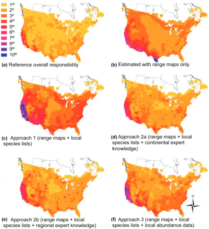
median increased from 0.11 to 0.19; Jmedian from 0.26 to 0.31; Smedian from 0.26 to 0.39) and overall responsibility (R² increased from 0.83 to 0.87; S from 0.47 to 0.69; and P from 0.67 to 0.75). It also corrected the tendency of estimates from range maps to largely overestimate reference values (slope ∼ 1) (Fig. 3b), and resulted in a more realistically detailed spatial pattern of estimated overall responsibility (Fig. 4c, b).
(Cantú-Salazar and Gaston 2013). In our particular analy-sis, high levels of omission errors are possibly an artifact of the smoothing used to construct the BBS abundance lay-ers resulting in a ‘spillage’ of predicted presence into cells where the species is absent (Sauer et al. 2007). This effect is likely higher in species with larger perimeter-to-area ratios, and so it may explain our finding that omission errors were more proportionately frequent in species with small ranges (S –0.90, p 0.001, Fig. 2b; see also example in Fig. 1).
Overall, the high rates of commission and omission errors we found reinforce calls for caution in the uncritical use of range maps as sources of data on the presence or absence of species at fine spatial scales (Hurlbert and Jetz 2007). Omission errors can affect the efficiency of conservation planning by biasing results towards known species occur-rences, potentially missing important areas where a species also exists. But commission errors are arguably even more problematic, if they lead to species being falsely believed conserved when they are not (Rodrigues et al. 2004a).
Value of range maps for estimating site responsibility
Overall responsibility estimated from range maps was gen-erally a good predictor (R² 0.83; Table 1, Fig. 3a) and captured the broad spatial patterns of reference values (Fig. 4a, b), even if estimates tended to largely overestimate reference values (slope 1). Agreement in relative order was less impressive (S 0.47), and a manager using solely range maps to prioritize between two sites would be wrong one out of three times (p 0.67).
Within most sites, estimates of specific responsibility obtained from range maps were weak predictors of reference values, in terms of order (Smedian 0.26) and even more so in terms of absolute values (R²median 0.11). For most sites, there was also little overlap between the top 25% species identified using estimated vs. reference values of specific responsibility (Jmedian 0.26). In other words, a site manager
0 10 20 30 40 50 0 1 2 3 4 5 6 7 8 9 0 20 60 100 140 180 220 260 0 20 40 60 80 100 0 10 20 30 40 50 0 1 2 3 4 5 6 7 8 9 (a)
Classes of species according to percentage of commission errors
Median range size (millions km
2
)
Median range size (millions km
2
)
(b)
Percentage of species Percentage of species
Classes of species according to percentage of comission errors
Figure 2. Histograms of the frequency of errors in species’ range maps, across the 316 species analyzed: (a) commission errors, percentage of sites from where the species is present according to the range maps, but absent according to the BBS data, in relation to the overall number of sites where present (according to the BBS data); (b) omission errors, percentage of sites from where the species is absent accord-ing to the range maps, but present accordaccord-ing to BBS data, in relation to the overall number of sites where present (accordaccord-ing to the BBS data). For both types, the histogram shows the percentage of all species (left y-axis) that fall into a particular 10%-class of error. We also present the median (and first and third quartiles) range size of the species in each class (black points and whiskers, right y-axis; measured as
than in the baseline Approach 1 (corresponding to m 1; Supplementary material Appendix 2, Table A2, Fig. A2). For m 8, there were marked improvements for all metrics comparing specific responsibility (R2
median increased from 0.19 to 0.42; Jmedian from 0.31 to 0.35; and Smedian from 0.39 to 0.45), in the spatial pattern of overall responsibil-ity (Fig. 4d) and in all but one metrics comparing overall responsibility (e.g. R2 increased from 0.87 to 0.94; S from 0.69 to 0.84). The only exception was a lowering of slope (from 1.01 to 0.80) indicating an increase in overestimation errors (Supplementary material Appendix 2, Fig. A2), and meaning that these estimates should be seen as informative for comparisons between sites, rather than as predictors of the real values.
Unfortunately, these results do not hold in the more plausible Approach 2b, whereby experts’ field experience is restricted to the regional scale: disappointingly, results were no better than those in the baseline Approach 1 (Table 1; Fig. 4e). This is because species’ relative abun-dances vary substantially across regions within their ranges However, this approach fails to highlight sites of
particu-larly high overall responsibility, underestimating by a factor of 2 or 3 those with the highest reference values (Fig. 3b). A site has an exceptionally high overall responsibility when it combines a high species richness (Supplementary material Appendix 1, Fig. A1a) and a prevalence of species with small global ranges (i.e. high mean site endemism; Supplementary material Appendix 1, Fig. A1b) and with high relative abundances in the site in relation to their abundances else-where (i.e., high mean species’ normalised local abundance; Supplementary material Appendix 1, Fig. A1c). Approach 1 combines information from the first two facets of responsi-bility, but not from the third. We explored ways of combin-ing the three in Approaches 2 and 3.
In Approach 2a, species of exceptionally high local abun-dance in the context of North American ranges (as iden-tified by simulated expert knowledge) were then given a higher weight (m 1) when estimating specific and over-all responsibility. For m values from 2 to 10, estimates of both specific and overall responsibility performed better
0 1 2 3 4 5 6 0 1 2 3 4 5 6 0 1 2 3 4 5 6 0 1 2 3 4 5 6 0 1 2 3 4 5 6 0 2 4 6 8 (a) (b) (c) (d) (e)
Estimated values of overall responsibility
Reference values of overall responsibility
Figure 3. Relationship between site values of overall responsibility as estimated under each approach and the reference values: (a) estimated from range maps only; the cloud of anomalous points in the lower right section of the scatterplot corresponds to southern Texas; (b) Approach 1 (range maps local species lists); (c) Approach 2a (range maps local species lists continental expert knowledge); (d) Approach 2b (range maps local species lists regional expert knowledge); (e) Approach 3 (range maps local species lists local abundances). Each point corresponds to a site. Sites for which estimated values match precisely the reference values fall over the black 1:1 line; points above correspond to underestimates and points below to overestimates. The red line was obtained from the linear regression model (forced through the origin) where estimated site responsibility is the predictor and reference responsibility is the response variable. Reference values of responsibility (y-axes) are more left-skewed towards lower values, an effect translated into the dominance of light colours in Fig. 4a.
In Approach 3 we simulated the effect of disregarding (assuming zero specific responsibility) the locally rare species in each site, i.e., those with a local abundance v. We found that for v 1, estimates of responsibility were much better than in Approach 1 (corresponding to v 0) and as good, or even better, than for Approach 2a (e.g. Smedian 0.67, compared with 0.39 in Approach 1 and 0.4 in Approach 2a; R² 0.95, compared to 0.87 in Approach 1 and 0.94 in Approach 2a; Table 1; Fig. 3e), and reproduced very (Sauer et al. 2007) and so a site may have exceptionally
high abundance of a species within the context of a region and yet be quite unexceptional across the species’ entire range. Unfortunately, these results suggest that relying on expert knowledge to provide a broader context to local species’ abundances is of little value if such knowledge is geographically restricted. This is thus an example of how adding more information does not necessarily result in bet-ter estimates.
Figure 4. Spatial patterns of overall responsibility across the study region. In (a) we present the reference values obtained from high-quality data on species abundances, the benchmark against which all other maps are compared. Other maps correspond to estimated values, obtained from: (b) species’ range maps only; (c) Approach 1 – a combination of range maps and local species lists; (d) Approach 2a – a combination of range maps and local species lists with expert knowledge of species abundance at the continental scale; (e) Approach 2b – as Approach 2a, but with expert knowledge of species abundance at the regional scale; (f) Approach 3 – combining range maps and local species lists and local data on species’ abundances. In each map, the color scale corresponds to 10 equal-interval classes.
the approaches we propose remain applicable, and making a good use of the available data is even more important in those circumstances.
Furthermore, we believe that our result that the range maps of more narrowly distributed species are generally less prone to commission errors (Fig. 2a) is likely to generalize more widely. Indeed, range boundaries can be drawn with higher accuracy if species are associated with particular geo-graphical features (e.g. islands, valleys, mountaintops) that can be mapped precisely. The maps of widespread species are also more likely to encompass wide areas of unsuitable habitat: for example, a widespread wetland species will be mapped over large territory encompassing much non- wetland habitat, whereas a restricted-range wetland species will be mapped into the specific wetland(s) where it is known to occur. Maps of restricted-range species are thus mapped with a higher precision, and accordingly they have previ-ously been used to pinpoint sites of particular importance to conservation, such as those identified by the Alliance for Zero Extinction (Ricketts et al. 2005), Key Biodiversity Areas (Langhammer et al. 2007), and highly irreplaceable protected areas (Le Saout et al. 2013). We thus predict that range maps can actually be very informative of site responsi-bility in regions with strong levels of endemism (e.g. Tropical Andes, Madagascar, southeast Asia; Stattersfield et al. 1998, Myers et al. 2000) and/or for taxa where range sizes are generally smaller (e.g. amphibians, whose median range size is 18 000 km2, contrasted with mammals, 250 000 km2; Baillie et al. 2004).
Conclusions and perspectives
The on-going global erosion of biodiversity (Butchart et al. 2010) is the cumulative result of myriads of impacts affect-ing species worldwide, mainly through the destruction and degradation of their habitats (Vié et al. 2009). Halting such erosion – as the World’s governments have committed to do (Secretariat of the Convention on Biological Diversity 2002, 2010) – requires a diversity of actions, not only dedicated conservation measures (e.g. protected areas) but also broader actions to mitigate the impacts of the human enterprise (e.g. of agricultural expansion, urbanisation, new infrastructure). The combined impact of these local actions relies therefore on the extent to which together they affect options for global biodiversity conservation. In the past few decades, the field of Systematic Conservation Planning developed rigorous methods for taking such broader context into account, in particular by focusing on the complementarity between sites (such that the value of a given site for conservation depends not only on what species are found at the site, but also on the species that occur elsewhere) and through the concept of irreplaceability (a measure of the extent to which options for conservation are lost if a site is lost) (Pressey et al. 1993, Ferrier et al. 2000, Wilson et al. 2010, Moilanen 2013). However, these methods are very data-hungry: a decision-maker wishing to apply them to inform decisions at the local scale would first require information on the distribution and abundance of species not only on its site of interest but across a much wider region. Here, we focused on approaches for allowing managers to make the best use of data plausibly well the spatial pattern of reference overall responsibility
(Fig. 4f). Nonetheless, absolute values of overall respon-sibility were systematically (and substantially) underesti-mated (slope 2.29; Fig. 3e), and so again these estimates should be seen as informative for comparisons between sites, rather than as predictors of the real values. The higher the abundance threshold v, the steeper the slope (the higher the underestimation errors), and for v 10, the estimates ceased from being better than in Approach 2a in terms of
R² and became progressively worse (Supplementary material
Appendix 3, Fig. A4). These results illustrate the advantages as well as the risks with this approach. Disregarding low abundance records improves responsibility estimates because in any given site it excludes those species that are locally rare but have large populations elsewhere (for which the site has little responsibility). However, it also excludes species that are rare everywhere, which may be in need of conservation attention in all sites where they occur. Accordingly, we found that increased v increased the number of species excluded from all sites where they occurred (Supplementary material Appendix 3, Fig. A4). This suggests that disregarding low abundance records may be an effective strategy for improving estimates of responsibility, but only for low thresholds v. Managers may also want to avoid excluding any species known to occur at low densities throughout their ranges.
Generalizability of the results
We investigated how species range maps such as those made freely available by the IUCN can inform local-scale conservations decisions. We have focused on the particular case of breeding land birds in North America because the exceptional BBS dataset allowed us to obtain high quality reference values of responsibility against which we could test different approaches for making the best use of data plausibly available to local managers. It is pertinent to ask whether the results we obtained can be generalized to other regions and to other taxa, i.e., whether managers working at local scales (of a similar order of magnitude as in our analyses: cell size ∼ 460 km2) but in other parts of the world and/or focused on other taxa would also find that range maps combined with local data provide a good basis for estimating the responsibil-ity of sites for global species conservation.
Species range maps are likely to be of lower quality (higher levels of commission and of omission errors) in regions with lower levels of expertise (e.g. in Africa; Rodrigues et al. 2010), particularly for the most diverse taxonomic groups (e.g. invertebrates, plants; Gaston and May 1992). Furthermore, in regions with a stronger human footprint (e.g. high defor-estation rates), species’ areas of occupancy may have become artificially patchy (e.g. restricted to remaining forest frag-ments), further increasing commission errors in range maps. The good estimates we found for birds in North America, even when using range maps alone (Table 1) are thus not necessarily generalizable to lesser-known taxa and/or in lesser-studied regions. Furthermore, even obtaining a com-plete local species list can be quite an ordeal in high-diversity areas (Lawton et al. 1998). But although these limitations are certain to reduce the quality of estimates of responsibility for hyper-diverse sites or taxa and in poorly known regions,
References
Baillie, J. et al. 2004. 2004 IUCN Red List of threatened species: a global species assessment. – IUCN.
Beresford, A. E. et al. 2011. Poor overlap between the distribution of protected areas and globally threatened birds in Africa. – Anim. Conserv. 14: 99–107.
Bibby, C. J. et al. 2000. Bird census techniques, 2nd ed. – Academic Press.
BirdLife International and NatureServe 2012. Bird species distribution maps of the world. – BirdLife International and NatureServe.
Bivand, R. and Lewin-Koh, N. 2010. maptools: tools for reading and handling spatial objects. – R package ver. 0.7-38. Butchart, S. H. M. et al. 2010. Global biodiversity: indicators of
recent declines. – Science 328: 1164–1168.
Cantú-Salazar, L. and Gaston, K. J. 2013. Species richness and representation in protected areas of the Western hemisphere: discrepancies between checklists and range maps. – Divers. Distrib. 19: 782–793.
Carwardine, J. et al. 2008. Cost-effective priorities for global mammal conservation. – Proc. Natl Acad. Sci. USA 105: 11446–11450.
Convention on Wetlands 1971. The Ramsar Sites Criteria.
– < www.ramsar.org/sites/default/files/documents/library/
ramsarsites_criteria_eng.pdf >.
ESRI 2012. ArcGIS 10.1 for desktop. – ESRI.
Ferrier, S. et al. 2000. A new predictor of the irreplaceability of areas for achieving a conservation goal, its application to real-world planning, and a research agenda for further refinement. – Biol. Conserv. 93: 303–325.
Gaston, K. J. 2003. The structure and dynamics of geographic ranges. – Oxford Univ. Press.
Gaston, K. J. and May, R. M. 1992. Taxonomy of taxonomists. – Nature 356: 281–282.
Gaston, K. J. and Fuller, R. A. 2009. The sizes of species’ geographic ranges. – J. Appl. Ecol. 46: 1–9.
Graham, C. H. and Hijmans, R. J. 2006. A comparison of methods for mapping species ranges and species richness. – Global Ecol. Biogeogr. 15: 578–587.
Heinrichs, J. A. et al. 2010. Assessing critical habitat: evaluating the relative contribution of habitats to population persistence. – Biol. Conserv. 143: 2229–2237.
Hurlbert, A. H. and Jetz, W. 2007. Species richness, hotspots, and the scale dependence of range maps in ecology and conserva-tion. – Proc. Natl Acad. Sci. USA 104: 13384–13389. IBAT 2015. Integrated biodiversity assessment tool. – BirdLife
International, Conservation International, IUCN, UNEP-WCMC, < www.ibatforbusiness.org >.
IUCN 2014. The IUCN Red List of threatened species. Version 2014.1. – Spatial data download, < www.iucnredlist.org/ technical-documents/spatial-data >.
IUCN and UNEP-WCMC 2012. The World Database on Protected Areas (WDPA). – IUCN and UNEP-WCMC.
Keller, C. M. E. and Scallan, J. T. 1999. Potential roadside biases due to habitat changes along breeding bird survey routes. – Condor 101: 50–57.
Knight, A. T. et al. 2011. Land managers’ willingness-to-sell defines conservation opportunity for protected area expansion. – Biol. Conserv. 144: 2623–2630.
Langhammer, P. F. et al. 2007. Identification and gap analysis of key biodiversity areas: targets for comprehensive protected area systems. – IUCN, IUCN World Commission on Protected Areas, James Cook Univ., AU, Rainforest CRC, AU.
Lawton, J. H. et al. 1998. Biodiversity inventories, indicator taxa and effects of habitat modification in tropical forest. – Nature 391: 72–76.
available to them at the local scale, while still taking into account the extent to which such decisions might affect global options for species’ conservation.
Freely available and covering an expanding diversity of taxa, the range maps collated under the IUCN Red List (IUCN 2014) are an increasingly valuable resource (Rodrigues et al. 2006), but given their coarse nature they are not necessarily in the radar of local managers as potentially useful sources of information. Our results sug-gest that despite their limitations, global range maps can indeed provide very valuable information to guide local conservation decisions in a global context, even more so if combined with local data plausibly available to manag-ers. We thus support calls for an urgent investments in the expansion of the geographic and taxonomic coverage of these data (Stuart et al. 2010). Refinement of species’ range maps through habitat suitability modelling, combin-ing local field records with environmental layers obtained from remote sensing (Rondinini et al. 2005, 2011), could further improve the relevancy of these maps for local decision-making.
Our results also reinforce the value of high quality local data obtained through fieldwork. We found that by combin-ing reliable occurrence data with range maps it was possible to eliminate the commission errors inherent to the latter and thus improve substantially site estimates of responsi-bility. We were able to go even further by differentiating among populations in each site and thus identify sites of particular importance for each species. Our results indicate that using expert knowledge to distinguish records of excep-tional abundance for each species can be a highly effective approach for doing so, but only in the unlikely scenario of experts’ field experience encompassing the species’ entire range. In contrast, discarding species of very low local abun-dance seems to be a more practical and effective method for improving the estimates of site responsibility based on plausible local data, but particular attention should be given to species of concern that occur in low densities throughout their ranges.
The approaches we propose here could be easily integrated into tools for supporting local-scale decision making, such as the Integrated Biodiversity Assessment Tool (IBAT 2015), complemented by information on other considerations that affect real-life conservation priorities (e.g. conservation costs, Carwardine et al. 2008; conservation opportunities, Knight et al. 2011; other biodiversity features besides species, such as ecosystem services, Naidoo et al. 2008). Approaches for improving the effectiveness of decision making are all the more urgent in hyper-diverse poorly-studied regions under high human pressure, where conservation-relevant decisions with truly global biodiversity impacts must proceed despite a paucity of biodiversity data.
Acknowledgements – We thank the North American Breeding
Bird Survey, BirdLife International and NatureServe for making species’ distribution data available, and to the thousands of peo-ple who contributed to their collection. We are grateful to Cyril Bernard for his technical support, and to Thomas Brooks and John Pilgrim for comments that have greatly improved the manuscript.
Rodrigues, A. S. L. et al. 2010. A global assessment of Amphibian taxonomic effort and expertise. – BioScience 60: 798–806. Rondinini, C. et al. 2005. Habitat suitability models and the
shortfall in conservation planning for African vertebrates. – Conserv. Biol. 19: 1488–1497.
Rondinini, C. et al. 2006. Tradeoffs of different types of species occurrence data for use in systematic conservation planning. – Ecol. Lett. 9: 1136–1145.
Rondinini, C. et al. 2011. Global habitat suitability models of ter-restrial mammals. – Phil. Trans. R. Soc. B 366: 2633–2641. Sauer, J. R. et al. 2007. The North American Breeding Bird Survey,
results and analysis 1966–2006. Version 10.13.2007. – USGS Patuxent Wildlife Research Center, < www.mbr-pwrc.usgs.gov/ bbs/ >.
Secretariat of the Convention on Biological Diversity 2002. COP 6 decision VI/26. Strategic plan for the convention on biological diversity. – Secretariat of the Convention on Biological Diversity.
Secretariat of the Convention on Biological Diversity 2010. Aichi biodiversity targets. COP 10 decision X/2: strategic plan for biodiversity 2011–2020. – Secretariat of the Convention on Biological Diversity.
Stattersfield, A. J. et al. 1998. Endemic bird areas of the world: priorities for biodiversity conservation. – BirdLife International. Stuart, S. N. et al. 2004. Status and trends of amphibian declines
and extinctions worldwide. – Science 306: 1783–1786. Stuart, S. N. et al. 2010. The barometer of life. – Science 328:
177–177.
Vié, J.-C. et al. 2009. Wildlife in a changing world – an analysis of the 2008 IUCN Red List of threatened species. – IUCN. Wilson, K. A. et al. 2010. Conserving biodiversity in production
landscapes. – Ecol. Appl. 20: 1721–1732. Le Saout, S. et al. 2013. Protected areas and effective biodiversity
conservation. – Science 342: 803–805.
Moilanen, A. 2013. Planning impact avoidance and biodiversity offsetting using software for spatial conservation prioritisation. – Wildl. Res. 40: 153–162.
Myers, N. et al. 2000. Biodiversity hotspots for conservation priorities. – Nature 403: 853–858.
Naidoo, R. et al. 2008. Global mapping of ecosystem services and conservation priorities. – Proc. Natl Acad. Sci. USA 105: 9495–9500.
Pompa, S. et al. 2011. Global distribution and conservation of marine mammals. – Proc. Natl Acad. Sci. USA 108: 13600–13605.
Pouzols, F. M. et al. 2014. Global protected area expansion is com-promised by projected land-use and parochialism. – Nature 516: 383–386.
Pressey, R. L. et al. 1993. Beyond opportunism: key principles for systematic reserve selection. – Trends Ecol. Evol. 8: 124–128.
Ricketts, T. H. et al. 2005. Pinpointing and preventing imminent extinctions. – Proc. Natl Acad. Sci. USA 102: 18497–18501. Rodrigues, A. S. L. 2011. Improving coarse species distribution
data for conservation planning in biodiversity-rich, data‐poor, regions: no easy shortcuts. – Anim. Conserv. 14: 108–110. Rodrigues, A. S. L. et al. 2004a. Effectiveness of the global protected
area network in representing species diversity. – Nature 428: 640–643.
Rodrigues, A. S. L. et al. 2004b. Global gap analysis: priority regions for expanding the global protected-area network. – BioScience 54: 1092.
Rodrigues, A. S. L. et al. 2006. The value of the IUCN Red List for conservation. – Trends Ecol. Evol. 21: 71–76.
Supplementary material (Appendix ECOG-02598 at < www. ecography.org/appendix/ecog-02598 >). Appendix 1–3.