Experimental validation of cooperative approach near road side units

HAL Id: hal-01130412

https://hal.archives-ouvertes.fr/hal-01130412

Submitted on 27 May 2016

HAL is a multi-disciplinary open access

archive for the deposit and dissemination of

sci-entific research documents, whether they are

pub-lished or not. The documents may come from

teaching and research institutions in France or

abroad, or from public or private research centers.

L’archive ouverte pluridisciplinaire HAL, est

destinée au dépôt et à la diffusion de documents

scientifiques de niveau recherche, publiés ou non,

émanant des établissements d’enseignement et de

recherche français ou étrangers, des laboratoires

publics ou privés.

Experimental validation of cooperative approach near

road side units

Koji Kamakura, Bertrand Ducourthial

To cite this version:

Koji Kamakura, Bertrand Ducourthial. Experimental validation of cooperative approach near road

side units. 10th IEEE International Wireless Communications & Mobile Computing Conference, Aug

2014, Nicosia, Cyprus. �10.1109/IWCMC.2014.6906493�. �hal-01130412�

Experimental Validation of Cooperative

Approach Near Road Side Units

Koji Kamakura

Department of Computer Science Chiba Institute of Technology Tsudanuma, Chiba 275–0016 Japan

Email: koji.kamakura@hds.utc.fr

Bertrand Ducourthial

Abstract—This paper reports an experimental validation of

the feasibility of cooperative approach for extending the coverage of vehicular-to-infrastructure (V2I) communication using our software platform named Airplug. Although the access time between a vehicle and a roadside unit (RSU) providing Internet access is limited in the real-world condition, our field trials demonstrate that it is extended by just passing by an RSU with forming a convoy of five vehicles installed Airplug. An overview of our software design and experimental setup is described, and discussed together with results using a WiFi access point (AP) as the RSU. Our field results show that the minimum of increased access time of our cooperative approach is always longer than the maximum of the access time of the single-vehicle case, even though the coverage varies.

I. INTRODUCTION

Many intelligent transportation system (ITS) applications rely on V2I communication to gather data produced by em-bedded sensors, calculators or emem-bedded applications. Most of these applications do not have strong constraints on the delay and on the messages losses, but on the other hand, the amount of data can be very large. For instance, applications willing to periodically collect data about the vehicle or environment status would not be easily damaged by few message loss or a few second delay, but process as much data as they can.

Although 802.11-based wireless networks in many

metropolitan areas around the world have been penetrated, the coverage is limited [1]–[3]. In [4], the median duration of connectivity at vehicular speeds is reported to be 13 seconds. Instead of deploying many RSUs with Wireless Access for Vehicular Environments (WAVE) [5], [6], custom-tailored for vehicular specific applications with an alternative network layer architecture, to cover the roads as it is planned in ITS architectures, such strategies should be considered which vehicles could collaborate to widen the coverage of an RSU. One strategy is the do-it-alone behavior: the vehicle stores the messages until encountering an RSU. This could increase the end-to-end delay of the messages from the vehicle to the destination in the infrastructure. On the one hand the message could never arrive, but on the other hand it could save the bandwidth because there is no vehicle-to-vehicle (V2V) communication for reaching the RSU. Another strategy is the cooperative behavior: the vehicle involves neighbors for sending its messages toward Internet. This approach could reduce the end-to-end delay compared to the do-it-alone one, but on the other hand it could generate many V2V messages. In some case, the network might be congested.

Our cooperative approach we will report here is imple-mented so that it could involve the benefits of the two

behaviors. Our goal is to measure how the coverage of an RSU is enlarged with our approach implemented. To this end, we details our implementation using AIRPLUG and explain how our field test was done with a WiFi AP as an RSU. To assess the coverage achieved, we define the access time as the creation time difference between the first and last messages arriving at the destination while the message source vehicle is passing by an RSU. Our field trials demonstrate that our cooperative approach extends the coverage of the RSU in terms of the access time.

The rest of this paper is organized as follows. In Section II, the software architecture we developed for this validation is described and then the methodology of the field trial and results measured are discussed in Section III. Section IV concludes the paper.

II. OVERVIEW OFEXPERIMENTALARCHITECTURE

A. Airplug

Our cooperative V2I architecture has been implemented using the Airplug software distribution [7]. This framework allows for easily developing protocols and distributed applica-tions, for studying them through emulation, and for developing them on target architecture (including embedded computers) without rewriting the code [8]–[10].

Airplugis a light message passing framework imposing very few conditions on the applications: writing messages on the standard output for sending, reading the standard input for receiving, and satisfying simple conventions of the text message exchange. Airplug applications can be designed using any language. In practice, most of our applications are implemented in Tcl/Tk for easing the deployment on both desktop and embedded PC and for a better integration in Network Simulator ns-2.

The Airplug software distribution is composed of appli-cations, libraries, and specific programs, depending on the mode of use: prototyping, emulation, and real deployment. Applications can exchange messages either locally or remotely following a publish/subscribe policy. The default behavior is to forward messages in the vicinity of a vehicle instead of learning on the neighborhood and exchanging addresses, which is resource consuming in a dynamic network. The cooperative V2I architecture also relies on such opportunistic approach [11]: no assumption is made on the existence of a complete end-to-end path from source to destination. Nodes do not require the global knowledge about network topology to forward a message. Routes are built dynamically wherein each node decides to forward or not the message based

Internet

RSU (WiFi

(a)Scenario of vehicles passing by an isolated RSU providing an Internet access

(b)Airplug architecture

Web Server (Apache)

AIRPLUG

Managed mode Ad-hocmode

TST GTW HOP

GPS

OS

V2V network V2I network (WiFi AP)

AIRPLUG

Ad-hoc mode Managedmode HOP GTW GPS OS Plugged process Local link Airplug process Operating system Network interfaces Web Server (Apache) AIRPLUG Ad-hoc mode Managedmode HOP

GTW GPS

OS AP)

Fig. 1. (a) Scenario of vehicles passing by an isolated RSU providing an

Internet access. (b) Airplug architecture: Red arrow shows a message flow when it is sent to the web server by the TST source node if it finds the AP via a network interface operating in managed mode. Blue arrows show a message flow when it is forwarded to other HOPs via a network interface operating in ad hoc mode if the source node does not find any AP. HOPs on different nodes receiving the message choose their behavior depending on whether their GTW finds an AP. If not, the message is forwarded the same way as the source node, as shown with blue arrows in the middle node. If

GTWdoes, the HOP forwards it to GTW and then it is sent to the AP via the

manage-mode interface, as shown with green arrows in the rightmost node.

on local information, implementing a store-carry-and-forward paradigm.

B. Airplug applications

We detail each application composing the cooperative V2I architecture in order to deliver messages from the source to the destination (web server) in our field trial.

The GPS application allows to receive GPS positions from a GPS receiver and to send them to all local applications that subscribed to them. In addition, positions are logged to be used when replaying the experiment in the network emulator of the Airplug distribution.

The TST application (TeST) generates messages to be sent to the infrastructure for the needs of the experiments. TST can subscribe to the local GPS application and then can receive the local position of the vehicle. Messages include timestamps that identifies when they are created at the source node and conformed to a given size and inter-packet gap (IPG). They are sent to the local GTW application (see Fig. 1(b)).

The GTW application (GaTeWay) is in charge of sending messages from local applications to the Internet. We implement two parameters dl and df, which are date for lifespan and

date before forwarding, respectively. GTW can send messages on TCP on a given web server. Every Tn seconds, GTW scans

networks to discover any gateway including RSU. Moreover, every Ts seconds, it processes the received messages, which

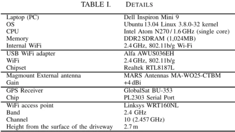
TABLE I. DETAILS

Laptop (PC) Dell Inspiron Mini 9

OS Ubuntu 13.04 Linux 3.8.0-32 kernel CPU Intel Atom N270 / 1.6 GHz (single core) Memory DDR2 SDRAM (1,024MB)

Internal WiFi 2.4 GHz, 802.11b/g Wi-Fi USB WiFi adapter Alfa AWUS036EH WiFi 2.4 GHz, 802.11b/g Chipset Realtek RTL8187L

Magmount External antenna MARS Antennas MA-WO25-CTBM Gain +4 dBi

GPS Receiver GlobalSat BU-353 Chip PL2303 Serial Port WiFi access point Linksys WRT160NL Band 2.4 GHz

Channel 10 (2.457 GHz) Height from the surface of the driveway 2.7 m

have been stored waiting for a network. In case a gateway is available, they are sent to the web server, or else dl and df

are decremented. When dl expires, the message is discarded.

When df expires, the message is forwarded to the local HOP

application. The delay parameters df and dlare counted every

Ts seconds. For instance, if Ts = 200 ms and df = 10, the

maximum time of a message buffered by GTW is 2 seconds. The HOP application deals with the V2V communication, based on the conditional transmission [11]. To avoid managing addresses which are very unstable in a dynamic network, a message is sent with two conditions. When the first one named CUP is true, HOP delivers the received message to the local application. When the second one named CFW is true, HOP forwards the received message to the vicinity of the node. Conditions can be very large and encompass addresses includ-ing geographic addresses for implementinclud-ing geocast, trajectory correlation to determine vehicles on the same lane, duration conditions or the availability of an Internet access (such as a close RSU) [10].

For the field trial, CUP and CFW are exclusive and simple. If the local GTW (GTW on the same node) has an interface connecting to a WiFi AP, CUP is true (i.e., CFW is false), or vice verse. If CUP is true, the message is forwarded to the local GTW and sent to the server via its interface (see the right node of Fig. 1(b)). If false, messages are forwarded to other nodes by HOP via the ad hoc mode interface (see the middle node of Fig. 1(b)).

III. FIELDTRIAL ANDRESULTS

A. Equipment

To measure the performance in realistic scenarios, we setup an outdoor field environment with five vehicles and a WiFi AP as an RSU. Each of the vehicles was equipped with an AIRPLUG-installed laptop PC, internal antenna, external antenna, and GPS receiver. In the PC, AIRPLUG runs on Ubuntu 13.04 with linux 3.8.0-32 kernel. The internal wireless interfaces of the laptops were used for association of the WiFi AP (managed mode) with GTW, and the external wireless interfaces were used for V2V communication (ad hoc mode) with HOP. The hardware details are listed in Table I.

B. Time Calibration

Consistency, rather than accuracy, of the system clock is needed for precise delay calculation between laptops and web server involved in the field test. Since laptops and servers are left to themselves, they would gain or lose time up to a few

TABLE II. TIMECALIBRATION

Node Tick Frequency Drift (ppm) Last offset (s) First offset (s) v1 9999 5821269 0.221 0.000031163 0.000604642 v2 10001 _−5604015 0.042 _{−0.000024584 −0.000088086} v3 10001 −5753498 −0.290 −0.000068095 −0.000100521 v4 10001 −5770689 0.188 −0.000027059 −0.000340140 v5 10001 −5445938 −0.123 −0.000014923 0.000351801 web 10000 3442123 −0.023 0.000010680 −0.000018161

hundred milliseconds per hour. To keep one common clock among them during the field trial, their system clocks were calibrated before the field trial, with Network Time Protocol (NTP) and the command adjtimex [12].

Even if their clocks are perfectly synchronized with NTP service, they will make their own drifts during the trial, in which they are off-lined. Such drifts will make wrong delay calculation in order of ms. While ntpd is running with a reliable time server, the daemon will then measure and record the intrinsic clock frequency offset in the so-called frequency file ntp.drift. After that the current frequency offset is written to the file at hourly intervals. Depending on the computer clock oscillator’s frequency error, this may take some hours or days to stabilize. When the value has converged, the frequency file contains the frequency offset measured in parts-per-million (PPM).

Therefore, with tick and frequency of the adjtimex command, the system clock was calibrated so that the ntp.drift should be less than 0.300 ppm, as listed in Table II. The last offset measured before the field trial and the first offset mea-sured after the trial are also listed (Note that the web server was always connected with the NTP server). Before the field trial, the minimum and maximum of the offset difference between the time server is 31.2 µs (v1) and−68.1 µs (v3), respectively; consequently, the maximum offset between the system clocks are 99.3 µs. After the trial (roughly 110 minutes after the last measure), the minimum and maximum differences are 604.6 µs (v1) and −340.1 µs (v4), respectively; the maximum offset difference among them are 944.8 µs. The delay can be calculated in error by less than one millisecond.

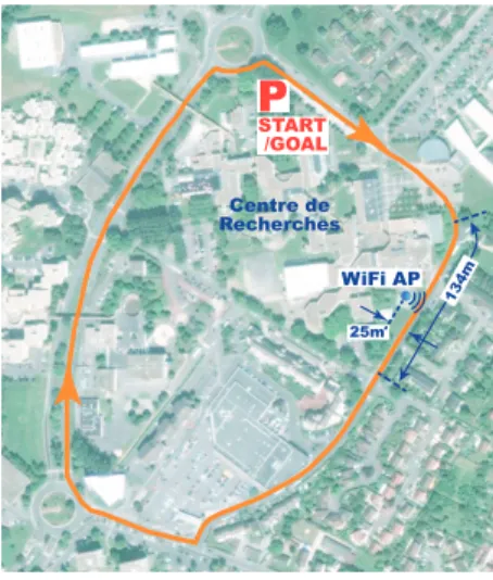
C. Driveway

Fig. 2 shows the driveway we used for the field trial. Vehicles passed by the WiFi AP located in the road side (25-m away from the driveway), at the speed of 35 km/h. Messages were generated by TST on the source node every second (IPG = 1000 ms) and sent by GTW on vehicular nodes toward the Web server via the AP. The AP is equipped with a DHCP server and secured using WPA2 Personal. It then assigns IP addresses after the authentication of the PC embedded in the vehicle, for which it took roughly 150-250ms. The 134-meter region shown in Fig. 2 was the coverage of the AP which was measured in a static situation with the internal antenna of the laptop. The driveway environment is so-called “sub-urban,” which 2- or 3-story buildings, trees, frequent traffic lights, and STOP signs, where steel fences exist between the AP and driveway. All trials were conducted in ambient traffic conditions with other vehicles present.

D. Basic scenario and Result

To measure the range of a WiFi AP on the sub-urban driveway, several rounds were carried out.

Centre de Recherches 13 4m 25m START /GOAL WiFi AP

P

Fig. 2. The driveway of our field trial is shown in orange, which has a

134-meter region measured in advance that the laptops were associated to the AP via their internal antennas in the static situation. The AP was located on the roof of the garage, which is 25 m away from the driveway.

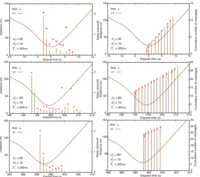
In Fig. 3, left three graphs show the delay of messages calculated from log files of the laptop and web server as a function of the elapsed time of the field trial, which is converted from UTC (Coordinated Universal Time) of the TSTmessage creation time. The right three graphs show the cumulative number of messages. The delay and the cumulative number are on the right-hand side axis. While, on the left-hand side axis of all the graphs, the distance of the vehicle (v1) from the AP calculated from the GPS track is shown with a brawn curve. The origin of the elapsed time is set to the instance at which the vehicle drove through the point closest to the AP for the first time. The top, middle, and bottom ones focus on part of the first, second, and third rounds, respectively, of the trial while the vehicle was approaching and leaving the AP. A red circle shows the amount of time taken for a TST message to be transmitted from v1 to the web server, and a brown vertical line under the red circle on the same point of the time axis shows the amount of time taken until the corresponding message was sent by GTW on v1 after it associated to the AP. The length of the vertical line does not include the propagation time for the message to travel over wireless channel from the sending interface of the vehicle to the receiver (AP) and over the wired network from the AP to the web server, and to be processed at the web server, including three-way hand shaking of TCP. Such times are understood through the gap between the circle and the line, because the plots of the delay performance (the left graphs) are depicted according to the creation time of TST message, a red circle and a vertical line at one point on the time axis correspond to one message created at the time. If there is no red circle over a vertical line, it means that the message did not reach the web server (i.e., lost), although it was sent by GTW.

We can see from the measured delay (left graphs) of Fig. 3 how long the access time was in the basic scenario. In the first round, the first and last messages received by the Web server were created at t =−2.7 and 7.9, respectively. The messages were created every second and ten consecutive circles are observed. Consequently, the access time from the vehicle to the AP for the first lap is 10 seconds. Putting it more precisely in terms of the creation time of TST message, the access time is 10.501 s. The average delay of the messages during the access time was 0.811 s. Similarly, the access times of the second

0 50 100 150 -15 -10 -5 0 5 10 15 0 5 10 15 D ist a n ce (m) C u mu la ti ve n u mb e r o f me ssa g e s 0 50 100 150 185 190 195 200 205 210 215 0 5 10 15 20 25 30 D ist a n ce (m) C u mu la ti ve n u mb e r o f me ssa g e s Elapsed time (s) Elapsed time (s) 0 50 100 150 380 385 390 395 400 405 410 0 5 10 15 20 25 30 35 40 D ist a n ce (m) C u mu la ti ve n u mb e r o f me ssa g e s Elapsed time (s) Elapsed time (s) Elapsed time (s) Elapsed time (s) dl = 60 df = 10 Ts= 200ms v1 Web dl = 60 df = 10 Ts= 200ms v1 Web dl = 60 df = 10 Ts= 200ms v1 Web dl = 60 df = 10 Ts= 200ms v1 Web dl = 60 df = 10 Ts= 200ms v1 Web dl = 60 df = 10 Ts= 200ms v1 Web 0 50 100 150 380 385 390 395 400 405 410 0 1 2 D ist a n ce (m) D e la y (se co n d ) 0 50 100 150 -15 -10 -5 0 5 10 15 0 1 2 D ist a n ce (m) D e la y (se co n d ) 0 50 100 150 185 190 195 200 205 210 215 0 1 2 D ist a n ce (m) D e la y (se co n d )

Fig. 3. Delay (left three graphs) and cumulative number (right three graphs)

of messages received by the web server (red circles) and sent by GTW of the vehicular (vertical lines) as a function of the elapsed time. Circles and vertical lines are depicted with the reception time of the corresponding TST messages.

and third rounds were 16 and 8 seconds from the middle and bottom graphs, respectively.

We can also see a tendency that the first two messages in the access time experienced slightly larger delay than the following messages for all the rounds. For example, the delays of the first and second messages were 2.071 s and 1.293 s, respectively, while the others were roughly 160–320 ms typi-cally, as shown in the bottom graph, although some messages were irregularly large without known reasons, like the eighth received message in the first lap and 11th and 14th received messages in the second lap. Such a large delay for the first few messages is certainly due to the route establishment measured at the application level (ARP, IP, DHCP recording update) and web application activation.

The right three graphs of Fig. 3 shows the cumulative number of messages received by the web server and sent by GTW of v1 of the basic scenario. Red circles and vertical lines are depicted according to the receiving time at the web server and sending time at GTW, respectively, unlike the delay performance shown in the left ones. Compared to a circle-line pair standing for a message (on the same time point) of the left graphs, the circle and line for the message in the right ones are shifted to the right along the time axis, depending on their delays. Red circles tend to be placed on the right side off the corresponding vertical lines because they are depicted over the vertical line in the left graphs. The offset between the red circle and vertical line along the time axis indicates the sum of the propagation and processing times on the way to and at the web server. For example, there is a vertical line at t = 5.9 in the top figure. Accordingly, the red circle corresponding to it is depicted almost on the vertical line at t = 6.9, which is the lower one among two red circles. This is confirmed from the gaps for the two messages generated at t = 5.6 and 6.6 in the left graph. The delay of the message at t = 5.6 is beyond one second (1.352 s) and larger than the one at t = 6.6 (0.249 s). This means that they arrived at the web

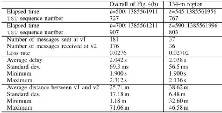
0 50 100 150 200 250 300 350 400 500 520 540 560 580 600 620 640 660 680 700 1.5 1.6 1.7 1.8 1.9 2 2.1 2.2 2.3 2.4 2.5 D e la y (se co n d ) Elapsed time (s) Elapsed time (s) 0 50 100 150 200 250 -20 -15 -10 -5 0 5 10 15 20 25 1.5 1.6 1.7 1.8 1.9 2 2.1 2.2 2.3 2.4 2.5 D ist a n ce (m) D ist a n ce (m) D e la y (se co n d ) v1 v2 v2 (HOP) v1 v2 v2 (HOP)

Fig. 4. The amount of time it took to be received by HOP on v2 and to be

sent by HOP on v1 (moving and leading vehicle) (vertical lines) as a function

of the elapsed time t, where 500≤ t ≤ 700.

server on almost the same time (i.e., the corresponding two red circles are placed at almost the same time axis). However, the cumulative number of messages received might jump by one message (or more) when we see it along the vertical axis. This means that the sequence number of TST message received were in disorder temporarily, but it would be corrected finally because the delayed messages were counted when they were received.

Note that in the right graphs, two vertical lines for the first two messages in the access time are depicted at almost the same point of the time axis (though it might be difficult to see them overlapping), since the difference between their delays has the tendency of one second.

E. Basic Scenario’s Summary

From Fig. 3, the total numbers of messages successfully received by the web server of the first, second, and third rounds are nine, sixteen, and eight, which are interpreted as 9-, 16-, and 8-second access time, respectively. Although GTW sent them eleven and seventeen times in the first and second rounds, respectively, the messages of the last sending attempts are not counted as the access time, because they were lost. On the other hand, the last sending attempt in the third round is counted because it reached the server. Such a failure happens when vehicular nodes moved out the range right before GTW had completed its sending process, despite of detecting the AP and initiating the sending process while it was on the boarder of the range.

We conclude from the results of the basic scenario that at maximum (second round), from the point of 50 m away from the AP, the vehicular node initiated communicating and ended

TABLE III. RESULT SUMMARY

Overall of Fig. 4(b) 134-m region Elapsed time t=500: 1385561911 t=545:1385561956

TSTsequence number 727 767

Elapsed time t=700: 1385561211 t=590: 1385561996

TSTsequence number 907 803 Number of messages sent at v1 181 37 Number of messages received at v2 176 36 Loss rate 0.0276 0.02702 Average delay 2.042 s 2.038 s Standard dev. 69.3 ms 56.5 ms Minimum 1.900 s 1.900 s Maximum 2.312 s 2.136 s Average distance between v1 and v2 25.71 m 38.62 m Standard dev. 17.18 m 6.48 m Minimum 1.18 m 32.60 m Maximum 71.06 m 46.58 m

its communication with the AP at the point of 100 m away, which is interpreted as the 16-second access time in terms of the generating time of TST message at maximum (the second round), while at minimum (the third round), from the point of 24 m away (the drive point closest to the AP) to the one of 60 m away, which is interpreted as the 8-second access time. F. V2V communication

The second scenario was carried out to measure the range of V2V communication, with two vehicles set up in the same way as in the basic scenario. V2V communication in our architecture is implemented as message exchange between HOP on different vehicles via their roof-mounted external antennas. Note that HOP used a wireless interface operating in the ad hoc mode.

In the V2V scenario, two cases were considered. The first one is that at the speed of 35 km/h, one vehicle labeled “v1” passed by another vehicle labeled “v2,” which stopped in the road side closest to the AP in order to measure one hop communication range with the roof-mounted ad hoc wireless connection. The second one is that v2 went together following five seconds behind of v1 to measure the loss rate of HOP-HOP communication in the driving situation.

Fig. 4 shows the delay of the V2V scenario as a function of the elapsed time, where the upper one depicts the first case and the lower one depicts the second one. Similarly to Fig. 3, vertical (brown) lines and red circles are shown, according to the creation time of TST message. The length of the vertical line shows the amount of time taken for a message to be created at v1 and to be sent by GTW on the source node. On the other hand, the red circle shows the amount of time taken for the message to be received by HOP on v2 from its creation time. Consequently, the gap between the red circle and brown line results in the amount of time spent between the two HOPs including the propagation time over the wireless channel. If there is no red circle over a vertical line at a time, it means that the message generated at that time did not reach v2 (for example, at t = 12.5, no red circle is over the vertical line). We observe that the first and last messages arriving at v2 were generated at t =−9.9 and 17.0, at which v1 was 88 m and 147 m away from the AP or 87 m and 121 m away from v2, respectively. In addition, we see that during the access time, among 25 sending attempts, 22 messages reached the server, where the loss rate is 0.12. The reason why the delay of the messages via the relay nodes are larger than two seconds is that they were buffered in GTW for df · Ts seconds before

being forwarded to its local HOP. We confirmed from the log

files that the processing time taken for messages from being forwarded by GTW to being sent by HOP were negligible (less than 1 ms).

In the lower one of Fig. 4, the delay measured in one of the rounds is shown, where v2 was driven so that it could follow five seconds behind v1. Since the distances shown are calculated from the AP, the gap between the brown and orange curves at one point of the time axis does not indicate the exact distance between them at that moment, the distance between v1 and v2 are summarized in Table III. As shown in the table, the loss rate during the elapsed time shown in the figure is 0.0276, which is much lower than the first case.

G. Cooperative approach

The third scenario is a five-vehicle scenario. Five vehicles were set up in the similar way to the basic scenario. Drivers drove their vehicles so that they should follow in the tracks of the vehicle ahead of them, with keeping the five-second delay, in particular in the 134-m region in front of the AP, shown in Fig. 2. Although they made a right turn at the corner right before entering the region, they got close to each other at the corner for braking, and afterward they tried to drive so that they could follow the vehicle ahead with the delay.

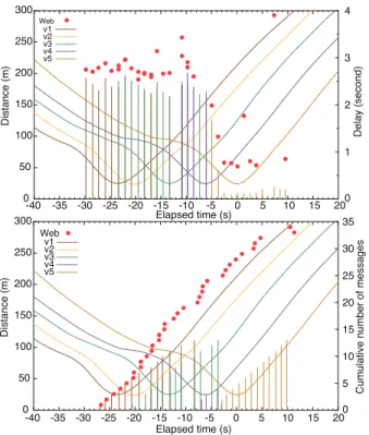
Fig. 5 shows the measured delay and cumulative number of messages as a function of the time of the five-vehicle scenario, where the last vehicle in the convoy was the source node generating messages and the other ones acted as the relay node. We can see from the upper graph that for 21 seconds from

t =−30 to −9, 17 messages reached the web server, though

the source node (v5) was 160 m or more away from the AP at t =−30, where it was out of the range from the results of the basic scenario. We confirmed from the log files that they were sent by v1, v2, v3, or v4. Two red circles are plotted on one point of the time axis, i.e., duplication reception. This is because vertical lines with different colors are depicted at those time points, which means that the message generated at the time point was sent by different nodes and they reached the server with the delay indicated as the gap in the figure. Duplication happened when a message sent by HOP was received multiple remote HOPs on different vehicles, which were in the range of the AP. From t =−5 to 10, messages sent by the source node (v5) reached the server because it was in the range of the AP. The delay exhibits the tendency that the first two messages sent by the source node experience a slightly large delay than the later ones (though the message generated at t = 7 experienced quite large delay of roughly 4 seconds).

In the lower one of Fig. 5, the vertical lines separated by color show the numbers of messages sent by individual nodes, and red circles show the number of messages received by the server. We observe that since v1 started connecting to the AP at t =−27, 24 messages in total reached the server before v5 (the source node) started sending, while seven messages were duplicated. Consequently, 17 messages are correctly re-ceived from the relay nodes. For the period of t =−6 to 10, ten messages were received from the source node. In short, 27 messages correctly reached the web server, and then the access time was increased by 17 seconds compared to the case without relay nodes.

Fig. 6 shows the measured delay and cumulative number of messages, where the middle vehicle (v3) was the source node. From the upper graph, we can see that for 21 seconds

0 50 100 150 200 250 300 -40 -35 -30 -25 -20 -15 -10 -5 0 5 10 15 20 0 5 10 15 20 25 30 35 D ist a n ce (m) C u mu la ti ve n u mb e r o f me ssa g e s Elapsed time (s) Elapsed time (s) v1 v2 v3 v4 v5 Web 0 50 100 150 200 250 300 -40 -35 -30 -25 -20 -15 -10 -5 0 5 10 15 20 0 1 2 3 4 D ist a n ce (m) D e la y (se co n d ) v1 v2 v3 v4 v5 Web

Fig. 5. Delay and cumulative number of TST messages received by the

web server (red circles) and sent by GTW of the vehicles (vertical lines) as a function of the elapsed time, whose origin is the time at which the TST-source node (v5) was closest to the AP.

from t =−23 to −7, 21 messages reached the web server,

with six duplicated receptions. In addition, four more messages reached the server from t = 12, which were sent by v5, where no duplication happened. Consequently, 19 messages reached the server via the relay nodes.

From the source node (v3), among 16 sending attempts, 13 messages were received with no duplication for the period from t =−6 to 11. The number of messages correctly received was increased by 19, compared to the single vehicle case.

We also see that the messages via the relay nodes were larger than the one directly sent by the source node. This is because of the buffering time of GTW. Since Ts= 200 ms, the

maximum buffering time was two seconds in the setting. Since messages sent by the relay nodes had been buffered for the two seconds in GTW on the source node before arriving at the relay nodes, their delay were greater than the buffering time. However, no GTW buffering happened on the relay nodes, because their HOPs forwarded messages to their GTW only if their wireless interface was associated. Such a delay could be reduced if using a smaller value of df, but more V2V messages

would have been generated (more cooperation, less do-it-alone behavior).

IV. CONCLUSIONS

In conclusion, our empirical measurement studies conclude that a line of five airplug-installed vehicles on the road achieves the extended access time of 27 seconds (corresponding to 145 m) at least, which is larger than the maximum access time of the single-vehicle case, 16 seconds (90 m). Our approach will be applied to various infrastructure such as cellular 2G/3G, WiMax, and IEEE 802.11p. We also confirmed the realism and versatility of the results of the emulation mode of AIRPLUG, which is useful for analyzing and optimizing the parameters

0 50 100 150 200 250 -25 -20 -15 -10 -5 0 5 10 15 20 25 30 0 5 10 15 20 25 30 35 40 45 D ist a n ce (m) C u mu la ti ve n u mb e r o f me ssa g e s Elapsed time (s) Elapsed time (s) 0 50 100 150 200 250 -25 -20 -15 -10 -5 0 5 10 15 20 25 30 0 1 2 3 4 D ist a n ce (m) D e la y (se co n d ) v1 v2 v3 v4 v5 Web v1 v2 v3 v4 v5 Web

Fig. 6. Delay and cumulative number of TST messages received by the

web server (red circles) and sent by GTW of the vehicles (vertical lines) as a function of the elapsed time, whose origin is the time at which the TST-source node (v3) was closest to the AP.

for the real situation, which is not mentioned because of space limitations.

ACKNOWLEDGMENT

The authors would like to thank P. Crubill´e, G. Dherbomez, P. Hudelaine, S. Bonnet, G. Sanahuja, and J. Radak for their help with the experiments.

REFERENCES

[1] J. Ott and D. Kutscher, “Drive-thru internet: IEEE 802.11b for

automo-bile users,” Proc. of IEEE INFOCOM2004.

[2] W. L. Tan, W. C. Lau, O.-C. Yue, and T. H. Hui, “Analytical Models and

Performance Evaluation of Drive-thru Internet Systems,” IEEE J. Select. Areas Commun., vol. 29, no. 1, pp. 207–222, Jan. 2011.

[3] V. B. C. da Silva, F. O. B. da Silva, M. E. M. Campista, “A

trajectory-based approach to improve delivery in drive-thru Internet scenarios,” Proc. of ICC 2013, Budapest, Hungary, pp. 489–494, June 2013.

[4] V. Bychkovsky, B. Hall, A. K. Miu, H. Balakrishnan, and S. Madden, “A

measurement study of vehicular Internet access using in situ Wi-Fi networks,” Proc. ACM MobiCom’06, Los Angeles, CA, Sept. 2006.

[5] 1609.1-5, WAVE Family Standards, IEEE Std.

[6] 802.11 Task Group p, IEEE Std.

[7] The Airplug Software Distribution [Online]. Available: https://www.hds.

utc.fr/airplug/doku.php

[8] A. Buisset, B. Ducourthial, F. El Ali, and S. Khalfallah, “Vehicular

net-works emulation,” Proc. of 19th ICCCN 2010, Zurich, Aug. 2010.

[9] B. Ducourthial and S. Khalfallah, “A platform for road experiments,”

Proc. of 69th IEEE VTC2009-Spring, Barcelona, Spain, April 2009.

[10] F. El Ali and B. Ducourthial, “A light architecture for opportunistic

vehicle-to-infrastructure communications,” Proc. of 8th ACM Mobi-wac 2010, Bodrum, Turkey, October 2010.

[11] B. Ducourthial, Y. Khaled, and M. Shawky, “Conditional transmissions:

Performance study of a new communication strategy in VANET,” IEEE Trans. on Vehicular Technol., vol. 56, no. 6, pp. 3348–3357, Nov. 2007.

[12] D. L. Mills, Network time protocol version 4 reference and

imple-mentation guide, [Online]. Available: http://www.eecis.udel.edu/∼mills/