Advances in Robust and Adaptive Optimization:
Algorithms, Software, and Insights
by
Iain Robert Dunning
B.E.(Hons), University of Auckland (2011)
Submitted to the Sloan School of Management
in partial fulfillment of the requirements for the degree of
DOCTOR OF PHILOSOPHY IN OPERATIONS RESEARCH
at the
MASSACHUSETTS INSTITUTE OF TECHNOLOGY
June 2016
c
○ Massachusetts Institute of Technology 2016. All rights reserved.
Author . . . .
Sloan School of Management
May 13, 2016
Certified by . . . .
Dimitris Bertsimas
Boeing Professor of Operations Research
Thesis Supervisor
Accepted by . . . .
Patrick Jaillet
Dugald C. Jackson Professor, Department of Electrical Engineering and
Computer Science
Co-director, Operations Research Center
Advances in Robust and Adaptive Optimization: Algorithms,
Software, and Insights
by
Iain Robert Dunning
Submitted to the Sloan School of Management on May 13, 2016, in partial fulfillment of the
requirements for the degree of
DOCTOR OF PHILOSOPHY IN OPERATIONS RESEARCH
Abstract
Optimization in the presence of uncertainty is at the heart of operations research. There are many approaches to modeling the nature of this uncertainty, but this thesis focuses on developing new algorithms, software, and insights for an approach that has risen in popularity over the last 15 years: robust optimization (RO), and its extension to decision making across time, adaptive optimization (AO).
In the first chapter, we perform a computational study of two approaches for solving RO problems: “reformulation” and “cutting planes”. Our results provide useful evidence for what types of problems each method excels in.
In the second chapter, we present and analyze a new algorithm for multistage AO problems with both integer and continuous recourse decisions. The algorithm oper-ates by iteratively partitioning the problem’s uncertainty set, using the approximate solution at each iteration. We show that it quickly produces high-quality solutions.
In the third chapter, we propose an AO approach to a general version of the process flexibility design problem, whereby we must decide which factories produce which products. We demonstrate significant savings for the price of flexibility versus simple but popular designs in the literature.
In the fourth chapter, we describe computationally practical methods for solving problems with “relative” RO objective functions. We use combinations of absolute and relative worst-case objective functions to find “Pareto-efficient” solutions that combine aspects of both. We demonstrate through three in-depth case studies that these solutions are intuitive and perform well in simulation.
In the fifth chapter, we describe JuMPeR, a software package for modeling RO and AO problems that builds on the JuMP modeling language. It supports many features including automatic reformulation, cutting plane generation, linear decision rules, and general data-driven uncertainty sets.
Thesis Supervisor: Dimitris Bertsimas
Acknowledgments
I would like to acknowledge and thank my supervisor Dimitris Bertsimas, who has been both a friend and mentor to me during my time at the ORC. I’ll always appre-ciate his patience during the early years of the degree, and his encouragement as I started to hit my stride. I am grateful to my doctoral committee members Juan Pablo Vielma and Vivek Farias, as well as Patrick Jaillet for serving on my general exami-nation committee and co-advising me during my first two years. I’m also grateful to Laura Rose and Andrew Carvalho for all their help over the years.
I must especially thank Miles Lubin for being a constant friend throughout the last four years, and an outstanding collaborator. I’d also like to thank Joey Huchette for joining us on our Julia-powered optimization mission, and all the Julia contributors at both MIT and around the world.
I’d like to thank everyone in my cohort for the conversations, the parties, the studying, and the support. I’d especially like to acknowledge John Silberholz, who has been an excellent friend and collaborator. I’d also like to acknowledge everyone who I worked with on the IAP software tools class, as well as all my co-TAs throughout the years. Special mention must go to Martin Copenhaver, Jerry Kung, and Yee Sian Ng, for all the conversations about life, the universe, and everything.
Finally, I’d like to acknowledge my family for their support not only during my time at MIT, but over my whole life – I would not be where or what I am today without them. I’d like to thank my friends David and Alec who have been supporting me for almost 15 years now – looking forward to many more. Last, but not least, I’d like to acknowledge my wife Kelly, who changed my life and makes it all worthwhile.
Contents
1 Introduction 15
1.1 Overview of Robust Optimization . . . 17
1.2 Overview of Adaptive Optimization . . . 21
1.3 Overview of Thesis . . . 22
2 Reformulation versus Cutting-planes for Robust Optimization 27 2.1 Introduction . . . 27
2.2 Problem and Method Descriptions . . . 30
2.2.1 Cutting-plane method for RLO . . . 31
2.2.2 Cutting-plane method for RMIO . . . 32
2.2.3 Polyhedral uncertainty sets . . . 36
2.2.4 Ellipsoidal uncertainty sets . . . 38
2.3 Computational Benchmarking . . . 39
2.3.1 Results for RLO . . . 42
2.3.2 Results for RMIO . . . 43
2.3.3 Implementation Considerations . . . 47
2.4 Evaluation of Hybrid Method . . . 50
2.4.1 Results for RLO . . . 51
2.4.2 Results for RMIO . . . 52
2.4.3 Implementation Considerations . . . 53
3 Multistage Robust Mixed Integer Optimization with Adaptive
Par-titions 59
3.1 Introduction . . . 59
3.2 Partition-and-bound Method for Two-Stage AMIO . . . 65
3.2.1 Partitioning Scheme . . . 66
3.2.2 Description of Method . . . 69
3.2.3 Calculating Lower Bounds . . . 73
3.2.4 Worked Example: Two-stage Inventory Control Problem . . . 74
3.2.5 Incorporating Affine Adaptability . . . 77
3.3 Analysis of the Partition-and-Bound Method . . . 78
3.3.1 Convergence Properties . . . 78
3.3.2 Growth in Partitioning Scheme . . . 80
3.4 Partition-and-Bound Method for Multistage AMIO . . . 83
3.4.1 Multistage Partitions and Nonanticipativity Constraints . . . 85
3.4.2 Multistage Method and Implementation . . . 88
3.5 Computational Experiments . . . 89
3.5.1 Capital Budgeting . . . 90
3.5.2 Multistage Lot Sizing . . . 92
3.6 Concluding Remarks . . . 97
4 The Price of Flexibility 99 4.1 Introduction . . . 99
4.2 Process Flexibility as Adaptive Robust Optimization . . . 103
4.2.1 Adaptive Robust Optimization Model . . . 104
4.2.2 Relative Profit ARO Model . . . 105
4.2.3 Solving the ARO Model . . . 108
4.2.4 Selecting the Uncertainty Set . . . 110
4.2.5 Extensibility of Formulation . . . 111
4.3 Pareto Efficiency in Manufacturing Operations . . . 113
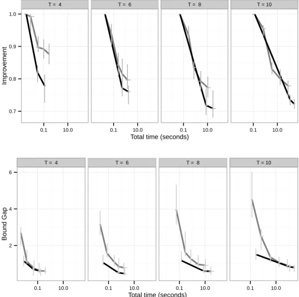
4.3.2 Relaxed Pareto Efficiency . . . 118
4.4 Insights from Computations . . . 119
4.4.1 Tractability of Adaptive Formulation . . . 120
4.4.2 Impact of Parameter Selections . . . 122
4.4.3 Utility of Pareto Efficient Designs . . . 126
4.4.4 Quality of Designs . . . 128
4.4.5 Price of Flexibility . . . 130
4.5 Concluding Remarks . . . 132
5 Relative Robust and Adaptive Optimization 135 5.1 Introduction . . . 135
5.2 Offline Problem is a Concave Function of Uncertain Parameters . . . 141
5.2.1 Reformulation of Robust Regret Problem . . . 142
5.2.2 Reformulation of Competitive Ratio Problem . . . 144
5.2.3 Integer Variables in Offline Problem . . . 145
5.3 Offline Problem is a Convex Function of Uncertain Parameters . . . . 147
5.3.1 Reformulating the Inner Problem as a MILO Problem . . . 148
5.4 Combining Objective Functions – Pareto-efficient Solutions . . . 151
5.4.1 Worked Example: Portfolio Optimization . . . 153
5.5 Computations and Insights . . . 155
5.5.1 Minimum-cost Flow . . . 156
5.5.2 Multistage Inventory Control . . . 162
5.5.3 Two-stage Facility and Stock Location . . . 166
5.6 Conclusions . . . 172
6 JuMPeR: Algebraic Modeling for Robust and Adaptive Optimiza-tion 177 6.1 Overview of JuMPeR . . . 180
6.1.1 Uncertain Parameters and Adaptive Variables . . . 182
6.1.2 Expressions and Constraints . . . 183
6.3 Case Studies . . . 188
6.3.1 Portfolio Construction . . . 189
6.3.2 Multistage Inventory Control . . . 191
6.3.3 Specialized Uncertainty Set (Budget) . . . 194
6.4 Comparisons with Other Tools . . . 199
A Notes for “Multistage Robust MIO with Adaptive Partitions” 203 A.1 Comparison of partitioning schemes for a large gap example . . . 203
A.2 Admissability of rule for enforcing nonanticipativity . . . 205
A.3 Comparison of partitioning schemes for multistage lot sizing . . . 206 B Reformulation of Stock Location Problem from “Relative Robust” 211
List of Figures
2-1 Performance profiles for RLO instances . . . 48 2-2 Performance profiles for RMIO instances . . . 49 2-3 Hybrid method runtimes . . . 54 3-1 Partitioning of simple uncertainty sets using Voronoi diagrams . . . . 69 3-2 Visualization of the partitions and active uncertain parameter tree
across multiple iterations . . . 71 3-3 Partitioning for Example 2 without adjustments for multistage case . 85 3-4 Partitioning for Example 2 with adjustments for multistage case . . . 89 3-5 Capital budgeting: partitions with iteration, and improvement versus
time . . . 91 3-6 Capital budgeting: improvement and bound gap versus time . . . 93 3-7 Multistage lot sizing problem: improvement and bound gap versus time 96 4-1 Examples of process flexibility designs . . . 101 4-2 Progress of a MIO solver for a flexibility instance . . . 122 4-3 Visualization of MIO gap versus time for flexibility problem . . . 123 4-4 Visualization of time to reach 90% MIO gap for flexibility problem . . 123 4-5 Parameters (Γ,𝐵) versus objective function value for “long chain” and
”dedicated” designs for flexibility problem . . . 125 4-6 Parameters (𝜌,𝐵) versus objective function value for “long chain” and
”dedicated” designs for flexibility problem . . . 126 4-7 Results for Pareto efficient designs for flexibility problem . . . 128 4-8 Effect of Γ for different levels of perturbation for flexibility problem . 130
4-9 Comparison with SAA designs for flexibility problem . . . 131
4-10 Price of flexibility for four different designs . . . 132
5-1 “Layered” minimum cost network with 𝐿 = 3,𝑀 = 3 . . . 159
5-2 “Layered” minimum cost network with optimal robust flows . . . 160
5-3 Empirical distribution of costs for “layered” minimum cost network . . 161
5-4 “Dense” minimum cost network with optimal robust flows . . . 162
5-5 Empirical distribution of costs for “dense” minimum cost network . . 163
5-6 Solve times for “layered” minimum cost network . . . 164
5-7 Objective function values for Pareto formulation of the inventory con-trol problem . . . 167
5-8 Performance in simulation for Pareto formulatino of the inventory con-trol problem . . . 167
5-9 Example instance of the two-stage facility and stock location problem 168 5-10 Solution times for the stock allocation problem . . . 170
5-11 Absolute robust performance in simulation for the facility location problem . . . 173
5-12 Competitive ratio performance in simulation for the facility location problem . . . 173
5-13 Robust regret performance in simulation for the facility location problem174 6-1 Overview of how JuMPeR interacts with related packages. . . 179
List of Tables
2.1 Problem classes for RO problem by uncertainty set . . . 39
2.2 Summary of RLO benchmark results for the polyhedral uncertainty set 42 2.3 Summary of RLO benchmark results for the ellipsoidal uncertainty set 42 2.4 Summary of RMIO benchmark results for the polyhedral uncertainty set 44 2.5 Summary of RMIO benchmark results for the ellipsoidal uncertainty set 45 2.6 Summary of RMIO benchmark results by root node treatment . . . . 46
2.7 Summary of RMIO benchmark results by root node treatment and feasibility . . . 46
2.8 Summary of RMIO benchmark results by heuristic usage . . . 47
2.9 Summary of hybrid method RLO benchmark results for the polyhedral uncertainty set . . . 51
2.10 Summary of hybrid method RLO benchmark results for the ellipsoidal uncertainty set . . . 52
2.11 Summary of hybrid method RMIO benchmark results for the polyhe-dral uncertainty set . . . 52
2.12 Summary of hybrid method RMIO benchmark results for the ellipsoidal uncertainty set . . . 53
3.1 Comparison of methods for the multistage lot sizing problem . . . 95
4.1 Results for Pareto efficient designs for flexibility problem . . . 129
Chapter 1
Introduction
Optimization in the presence of uncertainty is at the heart of operations research. The scope of these optimization problems is broad: from deciding how much of each crop to plant when future market prices are uncertain, to whether or not a coal-fired power plant should be run tomorrow given uncertainty in wind and solar power generation, to how much inventory should be ordered for future delivery when there is uncertainty in demand. Despite the importance of these problems, and the amount of effort dedicated to their solution, these optimization-under-uncertainty problems still represent a great challenge to solve in a variety of applications. George Dantzig, one of the fathers of operations research, wrote the following in an article in 1991:
“In retrospect, it is interesting to note that the original problem that started my research is still outstanding – namely the problem of planning or scheduling dynamically over time, particularly planning dynamically under uncertainty. If such a problem could be successfully solved it could eventually through better planning contribute to the well-being and sta-bility of the world.” [Dantzig, 1991]
This thesis does not claim to completely solve these problems, but instead provides a greater understanding of the relative merits of different solution techniques, presents new methods for some difficult classes of problems, explores their application to prob-lems of practical interest, and offers computer modeling tools to express them.
When addressing uncertainty in optimization problems, a decision maker must consider several things, including what information is available about the uncertain parameters, what computational resources can be applied, and what are the risk preferences for this situation. Examples of different types of information that may be available include past realizations of the uncertain parameters, a provided prob-ability distribution (possibly fitted to data, or perhaps from expert judgement), or a set of scenarios. The amount of computational resources available dictates, for a problem of a given size, what methods are available to use. For example, dynamic programming techniques can solve a wide variety of optimization-under-uncertainty problems “exactly”, but in general scale very poorly to larger problems (the “curse of dimensionality”). Finally, the risk preferences of a decision maker guide the types of objective functions and constraints we should use. For example, we may care mostly about the performance of a financial portfolio in expectation, or we may want to construct a portfolio that guarantees that it performs no worse than a certain factor relative to a benchmark. In an engineering application we may need to ensure that a constraint holds for all realizations of the parameters up to a certain limit, whereas in a power generation context we may only require that a constraint hold with a certain probability given a distribution for the uncertain parameters.
The temporal nature of the decisions may also be important to consider. If we are designing a structure that must not fail for a given set of realizations of the uncertain parameters, then a decision is made before the uncertainty is realized and the situation is resolved – the structure holds, or it does not. However, in many cases of interest in the operations research literature there are often (a sequence of) recourse decisions to be made. For example, we must decide how much of each crop to plant “here-and-now”, at the start of the season and before we know the market prices at the end of the growing season. Then, at the end of the season we make a “wait-and-see” decision of how much to sell with full knowledge of the market prices. In the case of controlling inventory for a retailer, we can model the ordering levels as a series of these “wait-and-see” decisions. Consider a setting where we make end-of-week orders: at the end of the first week, a “here-and-now” order must be made,
before demand for the next week is known. At the end of the next week, we now know the demand and make a “wait-and-see” decision – however, we still don’t know the demand for the weeks after that. This sequence of realizations and decisions is known as a multistage decision problem, and modeling that the decision at week 𝑛 is made with the benefit of knowing the uncertain parameters between now and week 𝑛 with certainty can dramatically increase the difficulty of these problems.
In this thesis, we focus on the robust optimization (RO) perspective of optimization-under-uncertainty. In Section 1.1, we provide a brief overview of what RO is, and how RO problems can be solved. In Section 1.2, we provide a similar overview of how RO has been applied to multistage decision problems, which we will refer to as adaptive RO (ARO) or simply adaptive optimization (AO). Finally, in Section 1.3, we provide an overview of the contributions of the following five chapters to the fields of robust and adaptive optimization.
1.1
Overview of Robust Optimization
While a comprehensive history of RO is beyond the scope of this introduction, we provide a general introduction to some of the key concepts here which are reinforced in the introductions to the individual chapters. For a broader overview, including key theoretical results and a summary of applications, we recommend the survey by Bertsimas et al. [2011a] and the book by Ben-Tal et al. [2009].
Robust optimization has taken a variety of forms over the past 30 years, but the key defining properties are that uncertain parameters in an optimization problem are modeled as belonging to an uncertainty set, and that we evaluate the feasibility and value of solutions with respect to the worst-case realization of the parameters over the uncertainty set. In the 1990s, much of the focus was on uncertainty in the objective function. The book by Kouvelis and Yu [1997] describes much of this work, which is primarily interested in combinatorial optimization problems. If the feasible set of solutions to a problem is 𝒳 , the uncertain parameters 𝜉 belong to an uncertainty set Ξ, the objective function is 𝑓 (𝜉, x), and 𝑓*(𝜉) is the objective function value you could
obtain with a priori knowledge of 𝜉, then the three variants on RO that Kouvelis and Yu [1997] consider are as follows:
∙ Absolute robust: maxx∈𝒳 min𝜉∈Ξ 𝑓 (𝜉, x)
∙ Robust deviation: maxx∈𝒳 min𝜉∈Ξ 𝑓 (𝜉, x) − 𝑓*(𝜉)
∙ Relative robust: maxx∈𝒳 min𝜉∈Ξ 𝑓 (𝜉,x)
𝑓*(𝜉)
The first, absolute robust, guarantees that we will do no worse than a certain absolute level of performance (e.g., “the portfolio return will not be worse than -2%”). The second, robust deviation, is also known as robust regret and attempts to incorporate that in many settings there exist values of the uncertain parameters for which no solution would have done well. The best any solution can achieve by this objective function is to have no (zero) regret, or colloquially, never leave anything on the table. The third, relative robust, is also known as competitive ratio and is very similar in spirit to the second. It guarantees our performance relative to some optimal benchmark: e.g., “the portfolio returns will not be worse than 90% of what we could have achieved”. The best any solution can achieve is a ratio of one, and although a solution that achieves this will also have zero regret, it is not the case that solution with minimal regret always has the best competitive ratio. Much of the work from this period used very simple uncertainty sets, often a “box” or “interval” set where each uncertain parameter was constrained to an interval. In Chapter 2 and Chapter 3 we focus on the absolute robust objective function, but we consider these relative notions in an application in Chapter 4, and explore in detail how to solve a wide variety of problems with these objective functions in Chapter 5.
In the late 1990s and early 2000s, a different line of research developed that was focused on absolute robustness, not only for objective functions but also for constraints. The general problem considered is
max
x∈𝒳 min𝜉∈Ξ 𝑓 (𝜉, x)
subject to 𝑔𝑖(𝜉, x) ≤ 0 ∀𝑖 ∈ ℐ, 𝜉 ∈ Ξ,
where 𝒳 captures deterministic constraints, 𝑓 is the objective function, 𝑔𝑖 are
con-straints, ℐ is an index set, and Ξ is the uncertainty set. Assuming that Ξ is not a finite set of discrete scenarios, which is uncommon, then this is a problem with an infinite number of constraints. We note that we can simplify the problem somewhat by moving the objective function into a constraint, and thus need only consider the treatment of uncertain constraints, i.e.,
max
x∈𝒳 ,𝑧 𝑧
subject to 𝑧 ≤ 𝑓 (𝜉, x) ∀𝜉 ∈ Ξ
𝑔𝑖(𝜉, x) ≤ 0 ∀𝑖 ∈ ℐ, 𝜉 ∈ Ξ,
(1.2)
Ben-Tal and Nemirovski [1999] considered this problem for the case where 𝑓 and 𝑔 are biaffine functions of x and 𝜉, or in other words, a linear optimization (LO) problem where the coefficients and bounds on the constraints may be uncertain parameters or affine functions of uncertain parameters. They show that, in the case where Ξ is an ellipse, the RO problem (1.2) can be reformulated to a problem with a finite number of constraints – although the resulting problem is a second-order cone opti-mization (SOCO) problem. This result doesn’t depend on x being continuous, so a mixed-integer LO (MILO) problem can also be reformulated to a mixed-integer SOCO (MISOCO) problem. However, at the time this work was done, solvers for MISOCO problems were not generally available and were not considered to be computationally practical. This problem was revisited by Bertsimas and Sim [2004], who considered a polyhedral uncertainty set instead of an ellipsoidal set. Their “budget” uncertainty set, which is used throughout this thesis, allows at most Γ uncertain parameters to deviate from their “nominal” values by a per-parameter “deviation”. A key benefit over the ellipsoidal set is that the resulting reformulation preserves linearity: a ro-bust LO problem is reformulated as a LO problem, and a roro-bust MILO problem is reformulated as a MILO problem.
Both these approaches use the theory of duality for convex optimization. We now briefly present the key idea of reformulation for RO, and simultaneously introduce an
alternative approach: cutting planes. Consider an uncertain constraint
𝜉𝑇x ≤ 𝑏 ∀𝜉 ∈ Ξ, (1.3)
with polyhedral uncertainty set Ξ = {𝜉 | F𝜉 ≤ g}. Suppose we have a ˆx that is feasible with respect to all other constraints, but not necessarily (1.3). As we cannot simply consider the infinite number of constraints on x here simultaneously, we will instead attempt to find a single ˆ𝜉 such that the resulting constraint is violated (i.e.,
ˆ
𝜉𝑇ˆx > 𝑏). As Ξ is a polyhedron, we can do so by solving the following LO problem:
max
𝜉 xˆ 𝑇𝜉
subject to F𝜉 ≤ g.
(1.4)
The process of finding a solution ˆx, adding new constraints by solving problem (1.4), then resolving for a new ˆx, is known as the cutting plane method. It is discussed at length in Chapter 2, and the general idea is used throughout this thesis. Returning to reformulation, observe that we can use LO duality (see, e.g., Bertsimas and Tsitsiklis [1997]) to formulate an equivalent dual problem
min
𝜋≥0 g
𝑇𝜋
subject to F𝑇𝜋 = ˆx.
(1.5)
We know that, for any feasible ˆ𝜋 and optimal solution ˆ𝜉 to the primal problem (1.4), the inequality g𝑇𝜋 ≥ ˆˆ x𝑇𝜉 holds. Thus, if we replace our original uncertain constraintˆ with the auxiliary constraints and variables
g𝑇𝜋 ≤ 𝑏 F𝑇𝜋 = x
𝜋 ≥ 0,
(1.6)
is at least the original left-hand-side’s worst-case value.
1.2
Overview of Adaptive Optimization
In Section 1.1, we focused on “single-stage” RO problems – that is, problems with no notion of sequential decision making. To motivate the difficulties that arise when considering multistage problems, consider a two-stage problem in which we first make a decision x, then uncertain parameters 𝜉 are revealed, and then we make another decision y, e.g.,
max
x min𝜉 maxy 𝑓 (𝜉, x, y). (1.7)
We can rewrite this problem in a similar form to the RO problem (1.1): max
x,y(𝜉) min𝜉 𝑓 (𝜉, x, y(𝜉)), (1.8)
where we can interpret maxy(𝜉) as optimizing over policies, i.e., functions of 𝜉. We
refer to problems such as these as adaptive RO (ARO) problems, or simply adaptive optimization (AO) problems, as the future decisions adapt as uncertain parameters are revealed.
The optimal policy y*(𝜉) may be very complicated (indeed, as we showed it here it is the solution of an optimization problem itself), and thus we might expect that this problem is not theoretically tractable in general. This was shown to be true by Ben-Tal et al. [2004], leading to a series of papers over the last decade attempting to find cases where it is tractable, to propose tractable approximations for the optimal policy, and to understand the behavior of those approximations. The first approximation was proposed in that same paper by Ben-Tal et al. [2004], where instead of a general y(𝜉) we use an affine approximation (or linear decision rule):
𝑦𝑗(𝜉) := ¯𝑦𝑗0+ 𝜉
𝑇y¯𝑗𝜉, (1.9)
massive simplification, but has shown to be very effective across a variety of settings – partly because its linearity keeps otherwise linear AO problems linear, but also because it has some theoretical backing (e.g., Bertsimas et al. [2010], Bertsimas and Goyal [2012]). A key failing of this approximation is its failure to accommodate discrete variables, which must necessarily be piecewise constant, not affine. Another approximation that has seen some success, and addresses the case of discrete variables, is finite adaptability [Bertsimas and Caramanis, 2010]. In finite adaptability, we first partition an uncertainty set Ξ, e.g. Ξ = Ξ1∪ Ξ2∪ · · · ∪ Ξ𝐾. We then define the policy
to be a piecewise constant policy, with a separate decision variable for each partition:
y (𝜉) = ⎧ ⎪ ⎪ ⎪ ⎪ ⎪ ⎨ ⎪ ⎪ ⎪ ⎪ ⎪ ⎩ ¯ y1, ∀𝜉 ∈ Ξ 1, .. . ¯ y𝐾, ∀𝜉 ∈ Ξ 𝐾. (1.10)
The key issue with this approach is how to decide the partitioning, and optimizing for the best 𝐾 partitions is a difficult optimization problem even when 𝐾 = 2. In Chapter 3, we propose a method that produces those partitions, applies the finite adaptability approach to multistage optimization, and incorporates affine adaptability to produce piecewise affine policies for continuous decisions. We also provide a more comprehensive survey in Section 3.1 of the various approaches to AO, including other extensions to affine and finite adaptability.
1.3
Overview of Thesis
This thesis consists of five chapters (apart from this introduction chapter). These are all based on papers submitted to, or accepted by, peer-reviewed journals, except Chapter 6 which describes an open-source software package for RO modeling.
Chapter 2: Reformulation versus Cutting-planes for Robust Optimization This chapter is based on Bertsimas et al. [2015b], which is published in Computational Management Science.
As briefly descried above in Section 1.1, there are two common ways to solve RO problems: reformulation (using duality), and using a cutting plane method. However, there is little guidance in the literature as to when to use each, and how to apply cutting planes to RO problems with integer variables. In this chapter, we precisely describe the cutting plane method for two popular uncertainty sets, including a con-sideration of how to integrate it into a branch-and-bound procedure. We then conduct a comprehensive computational experiment on a wide instance library, revealing that it is not clear that one method is uniformly superior to the other. Finally, we perform experiments that combine both methods, demonstrating that doing so can produce impressive performance. Cutting plane methods are used in many experiments in subsequent chapters, and the software described in Chapter 6 enables users to easily switch between cutting planes and reformulation.
Chapter 3: Multistage Robust Mixed Integer Optimization with Adaptive Partitions
This chapter is based on Bertsimas and Dunning [2016a], which is accepted for pub-lication in Operations Research.
Adaptive robust optimization is difficult, both in terms of computational prac-ticality and theoretical intractability. Despite this, practical approaches have been developed for many cases of interest. The most successful of these is the use of affine policies, or linear decision rules, where the value of future wait-and-see decisions is an affine function of uncertainty revealed previously. However, this approach fails when the wait-and-see decisions are discrete (integer, binary) decisions. In this chapter, we present a new approach to adaptive optimization that leads to piecewise constant policies for integer decisions, and piecewise affine policies for continuous decisions. It does so by iteratively partitioning the uncertainty set, and associating a different
decision with each partition. The solution of the problem with one set of partitions is then used to guide a refinement of the partitions – a procedure that can be repeated until the rate of improvement decreases, or the gap to the bound we describe falls below a tolerance. We provide theoretical motivation for this method, and charac-terize both its convergence properties and the growth in the number of partitions. Using these insights we propose and evaluate enhancements to the method such as warm starts and smarter partition creation. We describe in detail how to apply finite adaptability to multistage AMIO problems to appropriately address nonanticipativity restrictions. Finally we demonstrate in computational experiments using the JuMPeR software package (Chapter 6) that the method can provide substantial improvements over a non-adaptive solution and existing methods for problems described in the liter-ature. In particular, we find that our method produces high-quality solutions versus the amount of computational effort, even as the problem scales in both number of time stages and in the number of decision variables.
Chapter 4: The Price of Flexibility
This chapter is based on Bertsimas et al. [2015a], which has been submitted to Op-erations Research for review.
Process flexibility is a popular operations strategy that has been employed in many industries to help firms respond to uncertainty in product demand. However, additional flexibility comes at a cost that firms must balance against the reduction of risk it can provide. In this chapter, we reduce the price of flexibility by taking an optimization approach to the process flexibility design problem. Unlike many approaches previously discussed in the literature, we consider systems that may have nonhomogenous parameters and unbalanced capacity and demand. We formulate the problem as a robust adaptive optimization model, and propose a computationally tractable method for solving this model using standard integer optimization software. To further reduce the price we consider Pareto-efficient and relaxed Pareto-efficient robust solutions, and show that they correspond to flexibility designs that perform well in both worst-case and average-case demand scenarios. We demonstrate through
simulation experiments that our method can find flexible designs that reduce the price of flexibility by approximately 30% or more versus common flexibility designs, with a negligible impact on revenues and thus higher profits. We use JuMPeR (Chapter 6) for solving these problems.
Chapter 5: Relative Robust and Adaptive Optimization
This chapter is based on Bertsimas and Dunning [2016b], which has been submitted to INFORMS Journal on Computing for review.
Early approaches to RO focused on “relative” worst-case objective functions, where the value of a solution is measured versus the best-possible solution over an “uncer-tainty set” of scenarios. However, over the past ten years the focus has primarily been on “absolute” worst-case objective functions, which have generally been consid-ered to be more tractable. In this chapter, we demonstrate that for many problems of interest, including some adaptive robust optimization problems, that considering “rel-ative” objective functions does not significantly increase the computational cost over absolute objective functions. We use combinations of absolute and relative worst-case objective functions to find “Pareto-efficient” solutions that combine aspects of both, which suggests an approach to distinguish between otherwise very similar robust so-lutions. We provide reformulation and cutting plane approaches for these problems and demonstrate their efficacy with experiments on minimum-cost flow, inventory control, and facility location problems. These case studies show that solutions corre-sponding to relative objective functions may be a better match for a decision maker’s risk preferences than absolute.
Chapter 6: JuMPeR: Algebraic Modeling for Robust and Adaptive Op-timization
In the final chapter, we present “JuMPeR”, an algebraic modeling language for RO and ARO implemented as an extension to the JuMP modeling language. JuMPeR makes implementing and experimenting with ARO models fast and simple, providing features such as automatic reformulation, cutting plane generation, linear decision
rules, and complex uncertainty sets. We first present the overall design and structure of JuMPeR, before diving into some key implementation details. We then present three in-depth case studies, before finishing with a brief comparison with related tools.
Chapter 2
Reformulation versus Cutting-planes
for Robust Optimization
2.1
Introduction
Robust optimization (RO) has emerged as both an intuitive and computationally tractable method to address the natural question of how to handle uncertainty in optimization problems. In RO the uncertain parameters in a problem are modeled as belonging to an uncertainty set (see, e.g. Ben-Tal et al. [2009] or Bertsimas et al. [2011a] for a survey). A wide variety of uncertainty sets have been described in the literature, but polyhedral and ellipsoidal sets are by far the most popular types. Constraints with uncertain parameters must be feasible for all values of the uncertain parameters in the uncertainty set, and correspondingly the objective value is taken to be the worst case value over all realizations of the uncertain parameters. For this reason RO problems, in their original statement, typically have an infinite number of constraints and cannot be solved directly. The most common approach to date for solving them in the literature is to use duality theory to reformulate them as a deterministic optimization problems that may have additional variables, constraints, and even change problem class (e.g. a robust linear optimization (RLO) problem with an ellipsoidal uncertainty set becomes a second-order cone problem (SOCP) [Ben-Tal and Nemirovski, 1999]). Another method, used less frequently, is an iterative
cutting-plane method (e.g. Mutapcic and Boyd [2009]) that repeatedly solves a relaxed form of the RO problem with a finite subset of the constraints, checks whether any constraints would be violated for some value of the uncertain parameters, adds them if so, and re-solves until no violated constraint exists.
There is little guidance in the literature about which method should be used for any given RO problem instance. We are aware of one computational study by Fischetti and Monaci [2012] that directly compares the two methods for RLO and robust mixed-integer optimization (RMIO) problems with a polyhedral uncertainty set and finds that the cutting-plane method is superior for RLO and that reformulations are superior for RMIO. They do not attempt to indicate whether this result is statistically significant, and do not experiment with different variants of the cutting-plane method. Rather than just consider the question of which method is superior, we consider a different question in this chapter that we feel is more relevant for both practitioners and researchers, and acknowledges the ever-increasing popularity of parallel comput-ing. We draw inspiration from modern solvers such as Gurobi [Gurobi Optimization Inc., 2016] which, by default, simultaneously solve an LO problem with both the simplex method and an interior point method and return a solution whenever one of the methods terminates - effectively making the runtime the minimum of the two methods’ individual runtimes. This can naturally be extended to the RO case: we can solve an RO problem with both the reformulation method and the cutting plane method simultaneously, and the runtime is defined by the first method to finish. We do not implement in this chapter a general-purpose tool which does this simultaneous solve automatically, but the capability to do so would be a natural extension of the capabilities of an RO modeling system (such as the one described in Chapter 6).
The structure and contributions of this chapter are as follows:
∙ We provide a precise description of the application of the cutting-plane method to RMIO problems, including an identification of the added complexities over applying the method to RLO problems, and the variants that should be consid-ered by those seeking to implement the method.
∙ We replicate the findings of Fischetti and Monaci [2012] over an enlarged col-lection of instances, and extend them by evaluating the performance of the reformulation and cutting-plane methods for RO problems with ellipsoidal un-certainty sets. We use more appropriate metrics and employ statistical tech-niques to more precisely characterize the differences in performance between methods
∙ We enhance the performance of the cutting-plane method for RMIO problems by designing rules on when new cutting planes should be added, and evaluate a new heuristic to run alongside the MIO solver to improve runtimes.
∙ Finally we describe and evaluate our proposed hybrid method which uses both methods in parallel and stops when either method finishes. We discuss imple-mentation considerations and possible extensions.
Structure of the chapter. In Section 2.2, we detail the precise RO problem and uncertainty sets we evaluate. We discuss the details of the different cutting-plane algorithms and the possible variations in when new generated constraints should be added. We provide both the intuition and details for a new heuristic for RMIO problems. Section 2.3 explains the experimental setup, sources of data and the com-binations of instance, parameters, and methods we evaluated. We analyze the results in depth to compare the performance of the two methods and their variants on both RLO and RMIO problems. Section 2.4 investigates the proposed hybrid method’s performance relative to the individual methods and its implementation. Finally Sec-tion 2.5 summarizes the results.
2.2
Problem and Method Descriptions
We will consider the following general linear RO problem min 𝑐𝑇𝑥 subject to ˜𝑎𝑇1𝑥 ≤ 𝑏1 ∀˜𝑎1 ∈ 𝑈1 .. . ˜ 𝑎𝑇𝑚𝑥 ≤ 𝑏𝑚 ∀˜𝑎𝑚 ∈ 𝑈𝑚 𝑥 ∈ R𝑛1 × Z𝑛2,
where 𝑛1 and 𝑛2 are nonnegative integers, 𝑏1, . . . , 𝑏𝑚 are given scalars, 𝑐 is a given
vector, and 𝑈1, . . . , 𝑈𝑚 are the uncertainty sets for each constraint. We will denote
uncertain values using a tilde, e.g. ˜𝑎. In row 𝑖 a subset 𝐽𝑖 of the coefficients are said
to be subject to uncertainty, and all uncertain coefficients have a nominal value 𝑎𝑖𝑗
around which they may vary. We define the nominal problem to be the optimization problem identical to the above with the exception that all coefficients are at their nominal values with no uncertainty, that is ˜𝑎𝑖𝑗 = 𝑎𝑖𝑗 for all 𝑖 and 𝑗. Later in this
section we will detail the properties of the two types of uncertainty sets we consider in this chapter - the polyhedral set introduced in Bertsimas and Sim [2004] and the ellipsoidal set introduced in Ben-Tal and Nemirovski [1999]. These sets are both simple to describe but have substantially different deterministic reformulations and algorithms to calculate a new cutting-plane.
Before presenting the specific details of the polyhedral and ellipsoidal uncertainty sets (in Section 2.2.3 and Section 2.2.4 respectively) we will detail the cutting-plane methods we considered for both RLO problems and RMIO problems. While similar in spirit, there is a substantial difference in the details of their implementation. The method for RLO problems (Section 2.2.1) is fairly simple and comparable to other constraint generation methods. The method for RMIO problems (Section 2.2.2) re-quires consideration of exactly when in the integer optimization solution process cuts should be added.
2.2.1
Cutting-plane method for RLO
The idea behind the cutting-plane method for RLO is similar to other row generation methods such as Bender’s Decomposition. While there is a constraint for every ˜𝑎 in the relevant uncertainty set, only a small subset of these constraints is binding for a robust optimal solution. This suggests that only generating constraints as they are needed to ensure robustness of the solution would be an efficient technique. Given this motivation, the algorithm for RLO problems is as follows:
1. Initialize the master problem to be the nominal problem, that is the problem described in Eq. (2.1) where all ˜𝑎𝑖𝑗 are replaced with their nominal values 𝑎𝑖𝑗.
2. Solve the master problem, obtaining a solution 𝑥*.
3. For each uncertain row 𝑖 (that is, rows 𝑖 such that 𝐽𝑖 ̸= ∅)
(a) Compute ¯𝑎 = arg max˜𝑎∈𝑈𝑖˜𝑎𝑇𝑥*.
(b) If ¯𝑎𝑇𝑥* > 𝑏
𝑖+ 𝜖, add the constraint ¯𝑎𝑇𝑥 ≤ 𝑏𝑖 to the master problem.
4. If no constraints were added then we declare that 𝑥* is the optimal robust solution to the RO and terminate. If any constraints were added we return to Step 2.
The computational practicality of this method relies on the fact that while adding constraints will make the current master problem solution infeasible, we are able to hot-start the optimization (in Step 2) by using the dual simplex method. As a result almost all commercial and open-source LO solvers can be used to solve the master problem. We will defer discussing guarantees of the termination of this algorithm to Sections 2.2.3 and 2.2.4.
The constraint feasibility tolerance 𝜖 is a parameter that may be varied depend-ing on the needs of the application and the solver used, but should generally be an appropriately small value such as 10−6. We implemented the cutting-plane genera-tion and related logic in C++ and used the commercial solver Gurobi 5.6 [Gurobi Optimization Inc., 2016] to solve the master problem.
Note that a number of improvements to the classical cutting-plane method have been developed, including bundle methods and the analytic center cutting-plane method (ACCPM) [Briant et al., 2008]. These methods, in general, aim to “stabilize” the sequence of solutions 𝑥*, which can lead to improved theoretical and practical convergence rates. These techniques have been investigated in the context of stochas-tic programming [Zverovich et al., 2012] but to our knowledge not in the context of RO. Nevertheless, a preliminary implementation of a proximal bundle method did not yield significant improvements in computation time in our experiments, and the complexity of integrating these techniques within branch and bound (for RMIO) dis-couraged further investigation.
2.2.2
Cutting-plane method for RMIO
The cutting-plane method for RMIO is more complicated than the RLO case, al-though the principle of only adding constraints as needed is the same. The primary difference is that detailed consideration must be given to the most appropriate time to add new cuts, and that whatever timing is selected guarantees that the final solution is indeed robust.
Perhaps the most obvious place to add cuts is at the root LO relaxation in the branch-and-bound tree. However, it is not sufficient to apply the RLO cutting-plane method to just the root relaxation as the optimal robust integer solution may be affected by constraints that are not active at the fractional solution of the relaxation. Consider this simple example that demonstrates this behavior:
max 𝑥 subject to 𝑥 ≤ 1.5
𝑢 · 𝑥 ≥ 1 ∀𝑢 ∈ [0.9, 1.1] 𝑥 integer
The relaxed master problem for this RMIO consists of two constraints, 𝑥 ≤ 1.5 and 𝑥 ≥ 1 (taking the nominal value of 𝑢 to be 1), leading to the trivial solution 𝑥*𝑟𝑒𝑙𝑎𝑥 = 1.5 when we relax integrality. This solution is feasible to all constraints, so no new cutting planes are generated at the root. If we now branch once on the value of 𝑥 (i.e. 𝑥 ≤ 1 or 𝑥 ≥ 2) we will obtain the integer solution 𝑥 = 1 which is not feasible with respect to the uncertain constraint - in fact, there is no feasible integer solution to this problem. Although making the root relaxation feasible to the uncertain constraints doesn’t guarantee the feasibility of subsequent integer solutions, the addition of constraints at the root may guide the search along more favorable lines - we will analyze this effect in our computational results.
Another possibility is to check for and add new constraints at every node in the branch-and-bound tree, ensuring that the fractional solution at each node is feasible with respect to the uncertain constraints before further branching. This appears to have been the approach taken in Fischetti and Monaci [2012]. While this will ensure that any integer solution produced by branching will be feasible to the uncertain constraints, there is likely to be a heavy computational cost as we add cuts that are unnecessary, in the sense that they are being added to nodes on a branch of the search tree that may not produce an optimal integer solution or improve the bound.
A third possibility is to only check for and add new constraints when we obtain candidate integer-feasible solutions. These constraints are often described as lazy constraints as they are not explicitly provided to the solver before they are needed. Instead they are implemented by providing a callback to the solver that is responsible for checking the feasibility of all integer solutions and reporting any violated con-straints. The solver then discards the candidate integer solution (if it is not feasible) and adds the violated constraints to the active nodes of the branch-and-bound tree. Like adding constraints at each node, using lazy constraints is sufficient to guarantee that the final integer solution is feasible with respect to the uncertain constraints, but given the relatively small number of integer solutions for many MIO problems we decided that it would be a far more efficient method.
provable optimality before adding new constraints. If we wait until the end we are most likely to be adding useful constraints but we pay a huge computational cost as we essentially solve the master problem from scratch multiple times; unlike the case of RLO, no hot-start is possible as even the previous integer solution cannot be provided as an incumbent solution. Lazy constraints are a more appropriate technique as they are added before the solve is completed, allowing us to retain the bound corresponding to the fractional solution.
The final cutting-plane method we implemented is as follows:
1. As for RLO, initialize the master problem to be the nominal problem, that is the problem described in Eq. (2.1) where all ˜𝑎𝑖𝑗 are replaced with their nominal
values 𝑎𝑖𝑗.
2. Apply the RLO cutting-plane method to the root fractional relaxation of the RMIO master problem until the fractional solution is feasible with respect to all uncertain constraints. Note that while we may generate unnecessary cuts with respect to the final integer solution, we may also gain by requiring less cuts later on when we have progressed further down the tree.
3. The MIO solver now begins the branch-and-bound process to solve the master problem.
∙ Whenever an integer solution is found we will check all uncertain con-straints to see if any are violated by the candidate solution. If any viola-tions are detected we report these new lazy constraints to the MIO solver, which will discard the candidate integer solution. This ensures that only cuts active at integer solutions are added, and that any integer solution will be feasible with respect to the uncertain constraints. If no constraints are violated, the MIO solver will accept the integer solution as its incumbent solution, and the integrality gap will be evaluated relative to this solution. ∙ If we do find that the integer solution violates one of the uncertain con-straints, we will apply a heuristic that will try to obtain a feasible integer
solution using this candidate integer solution as a starting point. For more details, see Section 2.2.2.
We used Gurobi 5.6 [Gurobi Optimization Inc., 2016] to solve the MIO problem, with all other logic implemented in C++.
A heuristic to repair infeasible candidate integer solutions
The MIO solver will find multiple integer solutions as it attempts to solve the master problem to provable optimality. When it does so we will check whether any new constraints can be generated from the uncertainty sets that would make the candidate integer solution infeasible. If we do find any, we add these lazy constraints to the master problem and declare the found integer solution to be infeasible. The solver will discard the solution and keep on searching for another integer solution.
We hypothesize that in many cases these integer solutions that violated the un-certain constraints can be made feasible with respect to these constraints solely by varying the value of the continuous variables. The solver cannot explore this possi-bility by itself, as it is unaware of the uncertain constraints until we provide them. This may lead to possibly high-quality integer solutions being rejected and only re-discovered later in the search process. To address this issue we developed a heuristic that attempts to repair these integer solutions:
1. Our input is an integer solution 𝑥* to the master problem that violates one or more uncertain constraints. Create a duplicate of the master problem, called the subproblem.
2. Fix the values of all integer variables in the subproblem to their values in the integer solution 𝑥*. It follows that the subproblem is now equivalent to the master problem for a RLO problem.
3. Using the cutting-plane method for RLO problems to solve the subproblem. 4. If a solution to the subproblem is found, then this solution is a valid integer
deterministic. Report this solution to the MIO solver so that it may update its incumbent solution and bounds.
5. If no solution can be found for the subproblem then we take no action, and conclude that we must change the values of integer variables in order to obtain a robust integer solution.
We take a number of steps to improve the computational tractability of this heuris-tic. For example, we keep only one copy of the LO subproblem in memory and use it for all runs of the heuristic. This avoids the overhead of creating multiple copies, and we can use the dual simplex method to efficiently solve the subproblem given a new candidate solution. An additional effect is that we accumulate generated constraints from previous heuristic runs, further reducing the time for new integer solutions to be repaired or rejected. Secondly, we can take the lazy constraints we generate for the master problem and apply them to the heuristic subproblem to avoid re-generating them later. Finally all constraints we generate for the heuristic subproblem are valid for the master MIO, so we can add them to the master as lazy constraints to avoid generating integer solutions that will violate uncertain constraints in the first place.
The benefits of the heuristic are not guaranteed and may vary from instance-to-instance. The heuristic adds computational load that can only be made up for by improvements in speed with which we tighten the bound. In particular, by adding constraints back into the MIO master problem we may avoid needlessly generating non-robust integer solutions, but at the price of longer solve times at each node. We will explore these trade-offs between using the heuristic or not in Section 2.3.2.
2.2.3
Polyhedral uncertainty sets
We considered the polyhedral uncertainty set defined in Bertsimas and Sim [2004] with two properties: for a set 𝑈𝑖 corresponding to constraint 𝑖
∙ the uncertain coefficients ˜𝑎𝑖𝑗 ∀𝑗 ∈ 𝐽𝑖lie in the interval [𝑎𝑖𝑗 − ˆ𝑎𝑖𝑗, 𝑎𝑖𝑗 + ˆ𝑎𝑖𝑗], where
∙ at most Γ uncertain coefficients in the row are allowed to differ from their nominal value.
One may formulate a LO problem to find the coefficients ˜𝑎𝑖𝑗 ∈ 𝑈𝑖 that would
most violate the constraint ˜𝑎𝑇𝑖 𝑥 ≤ 𝑏𝑖. In Bertsimas and Sim [2004] the authors
demonstrate that duality theory allows us to replace the original uncertain constraint with a finite set of new deterministic constraints and auxiliary variables corresponding to the constraints and variables of the dual of this problem. As detailed in Table 2.1, this reformulation preserves the problem class of the original RO problem - a RLO problem becomes a LO problem, and likewise a RMIO problem becomes a MIO problem.
While we could generate new constraints by solving the aforementioned LO prob-lem, we can exploit the structure to solve the problem more efficiently by applying the following algorithm to each uncertain constraint 𝑖:
∙ Given a current solution 𝑥 to the master problem, calculate the absolute devi-ations 𝑧𝑗 = ˆ𝑎𝑖𝑗|𝑥𝑗| for all 𝑗 ∈ 𝐽𝑖.
∙ Sort 𝑧𝑗 (all non-negative by definition) from largest to smallest magnitude. The
indices 𝐽′ corresponding to the Γ largest values of 𝑧𝑗 will cause the maximum
violation of the constraint 𝑖 if set to their upper or lower bounds.
∙ If the constraint can be violated by setting those coefficients to their bounds while all other coefficients remain at their nominal values, add this violated constraint.
As we are only interested in a subset of the coefficients of size Γ this algorithm will run in 𝑂(𝑛 + Γ log Γ) time per constraint using an efficient partial sorting algorithm. We also note that many other polyhedral uncertainty sets exist that will require different cutting-plane algorithms, but we consider this set to be representative of many commonly-seen polyhedral sets in the literature. Termination of the plane algorithm is guaranteed in the case of the polyhedral uncertainty set: cutting-plane generation is equivalent to optimizing a linear function over a polyhedron, and there are only finitely many extreme points of the uncertainty set.
2.2.4
Ellipsoidal uncertainty sets
We evaluated the ellipsoidal uncertainty sets introduced in Ben-Tal and Nemirovski [1999, 2000], which model the coefficients ˜𝑎𝑖 ∈ 𝑈𝑖 as belonging to the ellipse
⎯ ⎸ ⎸ ⎷ ∑︁ 𝑗∈𝐽𝑖 (︂ ˜𝑎𝑖𝑗 − 𝑎𝑖𝑗 ˆ 𝑎𝑖𝑗 )︂2 ≤ Γ
The reformulation method for ellipsoidal sets replaces the uncertain constraints with new second-order cone constraints; thus LO problems become second-order cone prob-lems (SOCPs), and MIO probprob-lems become mixed-integer SOCPs (MISOCPs) (Ta-ble 2.1).
The algorithm to generate a new deterministic constraint for a given uncertain constraint is equivalent to finding the maximizer of a linear function over a ball, which has a closed-form expression. If we consider the Karush-Kuhn-Tucker conditions for the cutting-plane problem max˜𝑎∈𝑈𝑖˜𝑎
𝑇𝑥 we find that we can efficiently determine a
new constraint ¯𝑎 in 𝑂(𝑛) time by evaluating ¯ 𝑎*𝑗 = ⃦ Γ ⃦ ⃦ ˆ 𝐴𝑥 ⃦ ⃦ ⃦ ˆ 𝑎2𝑗𝑥𝑗 + 𝑎𝑗
where ˆ𝐴 is a diagonal matrix where the diagonal elements are the elements of ˆ𝑎. Note that this closed-form solution applies to generalizations which consider correlation matrices (non-axis aligned ellipses).
An interesting point of difference between the ellipsoidal cutting-plane method and the ellipsoidal reformulation is that the cutting-plane method does not modify the problem’s class as no quadratic terms appear in the generated constraints. However, unlike for polyhedral uncertainty sets, finite termination of the cutting-plane method applied to ellipsoidal uncertainty sets is not theoretically guaranteed, which perhaps discourages the implementation of this method in practice. Nevertheless, we will see that this method is indeed practical in many cases.
Table 2.1: Problem class of the deterministic reformulations and cutting-plane method master problems for RLO and RMIO problems, dependent on the choice of uncer-tainty set. The polyhedral set does not change the problem class. The cutting-plane method master problem remains in the same problem class as the original RO prob-lem regardless of the set selected, but the most efficient algorithm to generate a new cut is dependent on the set.
Polyhedral set Ellipsoidal set Robust Problem RLO RMIO RLO RMIO
Reformulation LP MIO SOCP MISOCP Cutting-plane master LP MIO LO MIO
Cut generation Sorting Closed-form
2.3
Computational Benchmarking
Obtaining a large number of diverse RO problems was achieved by taking instances from standard LO and MIO problem libraries and converting them to RO problems. We obtained test problems from four sources:
1. LO problems from NETLIB [Gay, 1985], all of which are relatively easy for modern solvers in their nominal forms.
2. LO problems from Hans Mittelmann’s benchmark library [Mittelmann]. 3. MIO problems from MIPLIB3 [Bixby et al., 1998].
4. MIPLIB 2010, the current standard MIO benchmark library [Koch et al., 2011]. We selected only the “easy” instances, where the nominal problem is solvable to provable optimality in under an hour.
Uncertain coefficients are identified using a procedure based on the method in Ben-Tal and Nemirovski [2000], that is similar to methods in other papers [Bertsimas and Sim, 2004, Fischetti and Monaci, 2012]):
∙ A coefficient is certain if it is representable as a rational number with denomi-nator between 1 and 100 or a small multiple of 10.
∙ It is otherwise declared to be uncertain, with a 2% deviation allowed from the nominal value: ˆ𝑎𝑖𝑗 = 0.02 |𝑎𝑖𝑗|
∙ All equality constraints are certain.
After removing all instances which had no uncertain coefficients, we were able to use 183 LO problems and 40 MIO problems.
We compared the reformulation and the cutting-plane methods for RLO (Sec-tion 2.3.1) and RMIO (Sec(Sec-tion 2.3.2). We tried three different values of Γ (1, 3, and 5) to test if the solution methods were sensitive to the amount of robustness. We used single-threaded computation throughout and a time limit of 1,000 seconds was enforced on all instances. All solver settings were left at their defaults unless otherwise stated.
For the case of the polyhedral reformulation for RLO problem we controlled for the choice between interior point (“barrier”) and dual simplex as the solution method. In particular, for the interior point method we disabled “crossover” (obtaining an optimal basic feasible solution) as we didn’t consider it relevant to the experiment at hand (the solution to the reformulation was not needed for any further use). The choice of solution method is significant in this case as we restricted the solver to one thread in all benchmarks - if multiple threads were available, we could use both simultaneously and take the faster of the two. This implication is explored further in Section 2.4.
We did not experiment with different solver options for the polyhedral set RMIO reformulation but did experiment with a solver option that chooses which algorithm to use to solve the ellipsoidal reformulation (a MISOCP). There are two choices available in Gurobi 5.6 : either a linearized outer-approximation, similar to the cutting plane method we employ, or solving the nonlinear continuous relaxation directly at each node. We solved the reformulation with each algorithm to investigate their relative performance for the RO problems.
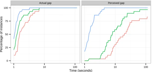
We use multiple measures to try to capture different aspects of the relative per-formance of the various methods and parameters. As the time to solve each problem varies dramatically we used only unitless measures, and avoided measures that are heavily affected by skew like the arithmetic mean employed in Fischetti and Monaci [2012]. We complement these numerical results with the graphical performance
pro-files [Dolan and Moré, 2002] which show a more complete picture of the relative runtimes for each method. Where possible we will relate the measures described below to these performance profiles.
The first and most basic measure is the percentage of problems solved fastest by each method. This corresponds to the 𝑦-axis values in the performance profiles for a performance ratio of 1. This measure is sensitive to small variations in runtime, especially for smaller problems, and does not capture any of the worst-case behaviors of the methods.
The second and third measures are both summary statistics of normalized run-times. More precisely, for a particular combination of problem class (RLO, RMIO), uncertainty set (polyhedral, ellipsoidal), and Γ we define 𝑇𝑀
𝑘 to be the runtime of
method 𝑀 for instance 𝑘 ∈ {1, . . . , 𝐾}, and define 𝑇𝑘* to be the best runtime for instance 𝑘 across all methods, that is 𝑇𝑘* = min𝑀𝑇𝑘𝑀. Then the second measure is,
for each method 𝑀 , to take the median of {︁𝑇𝑘𝑀 𝑇* 𝑘
}︁
. The median is a natural measure of the central tendency as it avoids any issues with outliers, although it is somewhat lacking in power when more than 50% of the instances take the same value, as is sometimes the case for our data. The third measure, which doesn’t have this short-coming, is to take the geometric mean of the same data for each method 𝑀 , that is to calculate (︃ 𝐾 ∏︁ 𝑘=1 𝑇𝑘𝑀 𝑇𝑘* )︃−𝐾 . (2.1)
We note that the arithmetic mean can give misleading results for ratios [Fleming and Wallace, 1986] and that the geometric mean is considered a suitable alternative.
A natural question is to ask how confident we are in the second and third measures, which we address with confidence intervals. To do so, we must frame our collection of test problems as samples from an infinite population of possible optimization prob-lems. We are sampling neither randomly nor independently from this population, so these intervals must be treated with some caution. As the distribution of these measures is not normal, and the sample sizes are not particularly large, we estimate 95% confidence intervals using bootstrapping (e.g. Efron and Tibshirani [1994]) which
Table 2.2: Summary of RLO benchmark results for the polyhedral uncertainty set for Γ = 5. % Best is the fraction of problems for which a method had the lowest run time. Median and Geom. Mean are the median and geometric mean respectively of the run times for each instance normalized by the best time across methods. The percentage best for the pseudo-method Reformulation (Best of Both) is calculated as the sum of the two reformulation percentages. The two entries marked with an asterisk represent a separate comparison made only between those two methods in isolation from the alternatives.
% Best Median (95% CI) Geom. Mean (95% CI)
Cutting-plane 75.5 1.00 (1.00, 1.00) 1.52 (1.31, 1.89) Reformulation (Barrier) 15.8 1.57 (1.40, 1.77) 1.88 (1.72, 2.10) Reformulation (Dual Simplex) 8.7 1.48 (1.40, 1.54) 1.69 (1.57, 1.85) Reformulation (Best of Both) 24.5 1.27 (1.20, 1.54) 1.39 (1.32, 1.49) Cutting-plane * 83.7 1.00 (1.00, 1.00) 1.39 (1.22, 1.68) Reformulation (Dual Simplex) * 16.3 1.42 (1.39, 1.54) 1.54 (1.46, 1.65) Table 2.3: Summary of RLO benchmark results for the ellipsoidal uncertainty set for Γ = 5. % Best is the fraction of problems for which a method had the lowest run time. Median and Geom. Mean are the median and geometric mean respectively of the run times for each instance normalized by the best time across methods.
% Best Median (95% CI) Geom. Mean (95% CI)
Cutting-plane 44.8 1.06 (1.00, 1.12) 1.76 (1.51, 2.18) Reformulation 55.2 1.00 (1.00, 1.00) 1.38 (1.27, 1.57)
avoids some of the assumptions that would otherwise have to be made to get useful results.
Finally we found that runtimes were relatively invariant to the choice of Γ. Any differences were less than the general minor variations caused by running the bench-marks multiple times. For this reason we present results only for Γ = 5 throughout the chapter. Additionally although we are not interested in comparing in any way the merits of polyhedral versus ellipsoidal sets, we wish to note that the relative “protection” level implied by a given Γ differs for the polyhedral and ellipsoidal sets.
2.3.1
Results for RLO
We found that the cutting-plane method was the fastest method for most (76%) RLO problems with polyhedral uncertainty sets (Table 2.2), which matches previous ob-servations [Fischetti and Monaci, 2012]. It also had a lower runtime geometric mean
than either of the two reformulation methods tried, although the difference is not substantial when viewed together with the confidence intervals. We also performed an alternative comparison between the dual simplex reformulation method and the cutting-plane method that again shows that the cutting-plane methods is faster on a vast majority of instances, but without a definitive difference in geometric mean. An explanation for this is to be found in Figure 2-1 which shows that the cutting plane method is within a factor of two of the fastest running time for approximately 90% of problems, but can be at least an order of magnitude slower than reformula-tion for the remaining 10%. Finally we have included a pseudo-method in Table 2.2 that takes the minimum of the two reformulation times, as many LO solvers can use both methods simultaneously. We see that while cutting-planes are still superior for a majority of problems, the geometric mean of the “best-of-both” reformulation method is lower than the cutting-plane method, although their essentially overlap-ping confidence intervals suggest not too much importance should be placed on this difference.
This result is inverted for RLO problems with ellipsoidal uncertainty sets, where the reformulation is superior in a small majority of cases (Table 2.3). Given this, it is unsurprising that there is essentially no difference in their median normalized running times. The geometric mean is more conclusive, with the reformulation method taking a clearer lead. This again seems to be due to significantly worse performance in a small number of instances, as evidenced by the performance profile in Figure 2-1.
2.3.2
Results for RMIO
For RMIO problems we have five major variations available: 1. Reformulation (in two minor variations for ellipsoidal sets).
2. Cutting-plane, without cutting-planes added at root node, heuristic disabled. 3. Cutting-plane, with cutting-plane method applied to root node, heuristic
Table 2.4: Summary of RMIO benchmark results for the polyhedral uncertainty set for Γ = 5. % Best is the fraction of problems for which a method had the lowest run time. Median and Geom. Mean are the median and geometric mean respectively of the run times for each instance normalized by the best time across methods. The two entries marked with an asterisk represent a separate comparison made only between those two methods in isolation from the alternatives.
% Best Median (95% CI) Geom. Mean (95% CI)
Cutting-plane 32.5 1.39 (1.00, 2.39) 2.96 (2.00, 5.26) Cutting-plane & root 20.0 1.19 (1.01, 1.41) 1.68 (1.40, 2.19) Cutting-plane & heur. 2.5 1.37 (1.07, 2.12) 2.92 (1.96, 5.23) Cutting-plane & root & heur. 7.5 1.22 (1.04, 1.55) 1.73 (1.43, 2.23) Reformulation 37.5 1.28 (1.00, 1.77) 1.88 (1.50, 2.68) Cutting-plane & root * 57.5 1.00 (1.00, 1.00) 1.58 (1.31, 2.07) Reformulation * 42.5 1.05 (1.00, 1.62) 1.76 (1.41, 2.56) 4. Cutting-plane, without cutting-planes added at root node, heuristic enabled. 5. Cutting-plane, with cutting-plane method applied to root node, heuristic
en-abled.
We now investigate in more details the relative benefits of generating constraints at the root node (Section 2.3.2) and of the heuristic (Section 2.3.2).
The results are summarized in Tables 2.4 and 2.5 for the polyhedral and ellip-soidal uncertainty sets respectively. For the polyhedral set we found that the various cutting-plane methods were fastest in 62.5% of instances, although there was little to separate the cutting-plane methods and reformulation in the medians. There was no meaningful difference in the geometric means with the notable exception of the two cutting-plane variants that did not add cuts at the root. We proceeded to simplify the comparison to just the cutting-plane method with cuts at the root and the refor-mulation. When viewed in this light there seems to be a slight edge to cutting-planes, but the difference is too small to confidently declare as significant. This contradicts the results in Fischetti and Monaci [2012] which concluded that cutting-planes were “significantly worse” than reformulation; this could be attributed to the enlarged test set, the addition of cutting planes at the root, the measurement metric used, or a combination of these factors.
![Figure 2-1: Performance profiles [Dolan and Moré, 2002] for RLO instances with polyhedral and ellipsoidal uncertainty, above and below, respectively](https://thumb-eu.123doks.com/thumbv2/123doknet/13887586.447208/48.918.219.698.118.945/figure-performance-profiles-instances-polyhedral-ellipsoidal-uncertainty-respectively.webp)
![Figure 2-2: Performance profiles [Dolan and Moré, 2002] for RMIO instances with polyhedral and ellipsoidal uncertainty, above and below, respectively](https://thumb-eu.123doks.com/thumbv2/123doknet/13887586.447208/49.918.222.696.137.937/figure-performance-profiles-instances-polyhedral-ellipsoidal-uncertainty-respectively.webp)