Advances in oxygen-17 NMR for biological structure determination

(1)

Advances in Oxygen- 17 NMR for Biological Structure Determination by

Eric George Keeler B.S., Chemistry, 2012 The Ohio State University

Submitted to the Department of Chemistry

in Partial Fulfillment of the Requirements for the Degree of DOCTOR OF PHILOSOPHY

IN PHYSICAL CHEMISTRY at the

Massachusetts Institute of Technology June 2017

MASSj49 A INTITUTE OF TECHNQOGY

JUL

0O6 2017

LIBRARIES

Signature redacted

Signature of A uthor .. ...---Department of Chemistry May4, 2017 Certified by ...

Signature redacted

0 ... Robert G. Griffin Professor of Chemistry Thesis Supervisor

Signature redacted

A ccepted by ... ... Robert W. Field Haslam and Dewey Professor of Chemistry Chairman, Departmental Committee on Graduate Students

(2)

This doctoral thesis has been examined by a Committee of the Department of Chemistry as follows:

Professor Moungi G. Bawendi...

Signature redacted

Chairman

Professor Robert G. Griffin

...

Signature redacted

Thesis Supervisor

Signature redacted

(3)

Advances in Oxygen- 17 NMR for Biological Structure Determination by

Eric George Keeler

Submitted to the Department of Chemistry

on May 12, 2017 in Partial Fulfillment of the Requirements for the Degree of Doctor of Philosophy in Physical Chemistry

ABSTRACT

The determination of the structures of biological systems, such as, fibril-forming peptides and proteins, membrane proteins, and viruses, by solid-state nuclear magnetic resonance (NMR) spectroscopy has materialized as an important field due to the high-resolution details that the technique provides. While solid-state NMR studies have focused on the three prevalent spin I= 1/2 nuclei present in biomolecules, oxygen has largely been ignored as a probe of the structure of such systems. Described in this thesis are the results of studies to advance the use of solid-state

170 NMR spectroscopy for structure determination of biological molecules by utilizing the

sensitivity of the electric field gradient (EFG) and chemical shift tensors of 17. We

demonstrated a distinct chemical shift range for bound water in crystalline amino acids and dipeptides and identified discordance between experimental and calculated EFG parameters. This difference was further studied via variable temperature 17 NMR experiments on barium chlorate monohydrate that demonstrated the effect of the librational motions of the bound water on the NMR measurable 170 quadrupolar coupling constant. A well resolved splitting in the 170

magic-angle spinning NMR spectrum was shown at the'rigid lattice limit of the bound water that was determined to be caused by the interaction between the 1H dipole coupling and the

'H-170 dipole couplings. Further study of bound water environments is presented exhibiting the

ability to resolve multiple unique bound water environments in a single system by high-resolution 170 NMR spectroscopy. We demonstrate the ability to utilize dynamic nuclear

polarization (DNP) NMR to polarize multiple nuclei via an endogenous radical dopant that does not disrupt the native crystal structure. Efficient "7 labeling of a dipeptide is explored to enable the study of the dipeptide via 70 NMR. Utilizing one- and two-dimensional double resonance

correlation spectroscopy, the interatomic correlations between oxygen and carbon, nitrogen, and hydrogen atoms were explored, exhibiting the ability of 170 NMR to determine structural characteristics of biomolecular solids. A study on the use of DNP NMR to study biosilica entrapped proteins is also presented as part of this thesis.

Thesis Supervisor: Robert G. Griffin Title: Professor of Chemistry

(4)

For my parents who constantly encouraged me, my grandparents who always believed in me,

my sister who looked out for me, and my wife who is always there for me.

(5)

ACKNOWLEDGMENTS

"If you hide your ignorance, no one will hit you and you'll never learn." Ray Bradbury, Fahrenheit 451

I would be remiss to think that I could acknowledge all of the people that have made my academic journey possible. I would first like to thank my advisor, Professor Robert G. Griffin for the opportunity to study under his guidance at MIT and the Francis Bitter Magnet Laboratory. I am grateful for the experiences that have been afforded me due to the guidance and support of Bob. Without Bob's support none of the research in this thesis would have been possible.

A very special thanks goes to Vladimir Michaelis for taking me under his wing when I first arrived at the FBML and guiding me through the years. Without his guidance and mentorship my years at the FBML would not have been nearly as productive or successful. Michael Colvin and Ta-Chung Ong also warrant recognition for their assistance throughout my time at the FBML. All my fellow Griffin Group members deserve thanks for the discussions and support that they provided me during my time there, including, Jennifer Mathies, Kevin Donovan, Sheetal Jain, Robert Silvers, Chen Yang, Kong Tan, Christy George, Yongchao Su, Marcel Reese, Evgeny Markhasin, Loren Andreas, Salima Bahri, Qing Zhe Ni, Cody Can, and Blake Wilson. A particular thanks to Dan Banks and Brian Michael for all the discussions that filled our office throughout the years. I must acknowledge the research and support staff of the FBML, Ajay Thakkar, Jeffrey Bryant, Mike Mullins, David Ruben, and Christopher Turner, as they have helped me to better understand and repair, from time to time, the hardware and

software required to perform my research.

The spark that ignited my journey into the world of solid-state NMR was Professor Philip J. Grandinetti. Without his direction into the complex universe of magnetic resonance I would not have reached such great heights. I would like to thank Professor Jay H. Baltisberger for his unending patience in teaching me and honing my skills as an experimental NMR spectroscopist. My time spent within the Grandinetti Group at Ohio State shaped my philosophy as an NMR spectroscopist and I will never forget all the great discussions with Brennan Walder, Derrick Kaseman, and Kevin Sanders. Thank you all for exposing my ignorance and allowing me to grow as a person and a spectroscopist.

Without all the love and encouragement of my family I would not be where I am today. My parents, Jeffery and Kristina Keeler, nurtured my curiosity and encouraged me to pursue my dreams and without them I would not have achieved half of what I have. My sister, Danielle, has always been there as a constant example throughout my life. To my wife, Alexandra, without your love and reassurances I would never have reached this mountaintop. I hope that we continue to bring out the best in one another as we continue to reach for our wildest dreams! To my brother-in-law, Ray, our stimulating intellectual discussions have had an immeasurable effect on expanding my scientific and critical thinking. To my extended family, particularly my uncle and aunt, Duane and Jane, and my wife's family, Steve, Mary, Matt, Amanda, and Michael, I thank you from the bottom of my heart for your constant support and patience when I talk about my research!

(6)

(7)

List of Figures

Figure 1.1. Energy diagram for the Zeeman interaction for a spin I= 1/2...17

Figure 1.2. Vector representation of magnetic resonance...18

Figure 1.3. Visualization of the MAS rotor spinning at the magic angle ... 20

Figure 1.4. Haeberlen (a,b) and Herzfeld-Berger (c) CSA conventions demonstrated on a CSA p ow der p attern ... 24

Figure 1.5. Diagram demonstrating the nuclear charge distribution of the magnetic dipole moment (a) and the electric quadrupole moment (b) ... 28

Figure 1.6. The energy level diagram for a spin 1=5/2 nuclei for the Zeeman interaction with the first and second order correction of the quadrupolar interaction ... 30

Figure 1.7. Simulated 170 NMR spectra for Ba(C10₃)₂-H₂1 70: stationary (a), fast sample spinning about 54.74' (b), and fast sample spinning about 70.12' (c) ... 33

Figure 1.8. Energy level diagram for a two-spin (one electron and one nucleus) system...37

Figure 1.9. Energy level diagram for a three-spin (two electrons and one nucleus) system ... 38

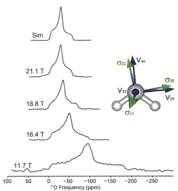
Figure 2.1. 170 NMR of L-asparagine-H₂0 at 16.4, 17.6, and 21.1 T ... 56

Figure 2.2. 170 MAS NMR of sodium L-aspartic acid monohydrate ... 57

Figure 2.3. 170 MAS NMR spectrum of three resolved oxygen sites present in L-cy steine -H C l-H 20 ... 59

Figure 2.4. 170 MAS NMR of L-glycyl-glycine HC1 monohydrate ... 60

Figure 2.5. 170 experimental and GIPAW-calculated quadrupolar coupling constants (a) and asym m etry param eters (b) ... 65

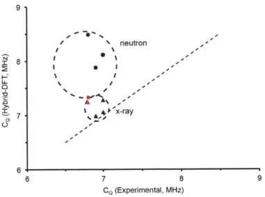
Figure 2.6. Relationship of calculated (hybrid-DFT) vs experimental CQ ... 68

Figure 2.7. 170 chemical shift ranges (green, e) and MAS simulations ... 70

Figure 2.8. Experimental and GIPAW-calculated '70 isotropic chemical shift (a), span (b), and skew (c) for bound water in the amino acid monohydrates...71

Figure 2.9. Relationship between HOH bond angle and average O-H bond distance (from GIPAW optimized crystalline structures) and GIPAW (a) and experimentally (b) determ ined 170 isotropic chem ical shift... 73

Figure 2.S1. ASN neutron crystal structure using various treatments to test GIPAW convergence criteria ... 77

Figure 2.S2. 170 nonspinning NMR spectra of sodium L-aspartic acid monohydrate ... 78

Figure 2.S3. 170 MAS NMR (21.1 T) of L-arginine -HCl- H20...78

Figure 2.S4. 170 nonspinning (left) and MAS (right) NMR of L-histidine -HCl- H20 ... 79

Figure 2.S5. 17 0 nonspinning NMR spectrum of L-cysteine -HCl- H20...79

Figure 2.S6. 17 0 nonspinning (left) and MAS (right) NMR of L-glycylglutamine -H20...80

(11)

Figure 2.S8. Hybrid-DFT crystal structure convergence for single molecular unit without all

atom op tim ization ... 82

Figure 2.S9. Hybrid-DFT crystal structure convergence for single molecular unit with all atom op tim izatio n ... 82

Figure 2.S 10. Hybrid-DFT crystal structure convergence for extended structures ... 83

Figure 2.S 11. 170 experimental and calculated (GIPAW) quadrupolar coupling constants ... 83

Figure 2.S 12. 10 experimental and calculated (GIPAW) quadrupolar asymmetry parameters ... 84

Figure 2.S 13. 170 experimental and calculated (GIPAW) isotropic chemical shifts...84

Figure 2.S14. Relationship between 170 NMR chemical shift (ppm) and O-H bond distance from X-ray and neutron structures (a), H-0-H bond angle from X-ray and neutron structures (b), and H20---NH 3 distance... 85

Figure 2.S15. The relationship between: experimental 170 quadrupolar coupling constant (a), experimental 170 quadrupolar asymmetry parameter (b), GIPAW calculated 170 quadrupolar coupling constant (c), GIPAW calculated 170 quadrupolar asymmetry parameter and the hydrogen bond distance between the amine functional group and water molecule (i.e., H₃N---OH2) from crystalline data (d)...86

Figure 2.S16. Simulated "70 nonspinning NMR of ASN...87

Figure 3.1. Molecular and long-range crystal packing of Ba(Cl03)2-H20 ... 101

Figure 3.2. MAS and stationary 170 NMR spectra of Ba(Cl0 3)2 H21 70...106

Figure 3.3. The EFG and CSA tensor components taken from GIPAW calculations...109

Figure 3.4. 170 V T M A S N M R spectra...111

Figure 3.5. 170 M A S N M R spectra at 105 5 K ... 113

Figure 3.S1. 170 MAS NMR spectra and simulations of Ba(C103)2 H20...117

Figure 3.S2. RAPT profile of Ba(C03)2-H2170 ... 118

Figure 3.S3. Stationary 10 NMR spectra and simulations of Ba(Cl0 ₃)2-H20 ... 119

Figure 3.S4. Experimental stationary 'H NMR spectrum (a) and simulation (b) of B a(C l0 3)2 H 20 at 16.4 T ... 120

Figure 3.S5. Stationary 'H NMR spectra and simulations of Ba(Cl03)2 H20 at 5 T ... 121

Figure 3.S6. Experimental (a) and simulated (b-g) 170 MAS spectra of Ba(C103)2-H2170 ... 122

Figure 3.S7. Plots of the refined structure calculations using GIPAW that relate the O-H distance to calculated CQ (a) and calculated iQ (b) ... 123

Figure 3.S8. Plots of the refined structure calculations using GIPAW that relate the LHOH angle to calculated CQ (a) and calculated rjQ (b)...124

Figure 3.S9. Plots of the refined structure calculations using GIPAW that relate the H-0(2) distance to calculated CQ (a) and calculated r- (b)...125

Figure 4.1. M olecular unit of LM N crystal structure...137

(12)

Figure 4.3. Experimental 170 2D M QM AS spectra...147

Figure 4.4. Experimental (left) and simulated (right) 2_{H stationary spectra of LMN ... 148}

Figure 4.5. 15N CPMAS (a) and direct (b) NMR spectra of LMN at 11.7 T ... 149

Figure 4.6. 15N experimental (solid) and simulated (dashed) NMR spectra of LMN ... 150

Figure 4.7. 'H DNP enhanced, non-DNP-enhanced spectra, and DNP enhancement profiles.... 152

Figure 4.8. 15N DNP enhanced, non-DNP-enhanced spectra, and DNP enhancement profiles ..154

Figure 4.S1. Experimental 170 2D MQMAS spectrum at 18.8 T...156

Figure 4.S2. Experimental 10 2D MQMAS spectrum at 21.1 T...156

Figure 4.S3. Sim ulated 170 2D M QM AS spectra...157

Figure 4.S4. RA PT profile of LM N at 21.1 T ... 158

Figure 4.S5. Comparison of sensitivity enhancement techniques for '70 MAS NMR ... 158

Figure 4.S6. Experimental (a,b) and simulated (c) 17 stationary NMR spectra ... 159

Figure 4.S7. Experim ental 170 stationary spectra...160

Figure 4.S8. 'H microwave power dependence (a) and build-up time (b) at 5.01474 T ... 161

Figure 4.S9. 1N DNP-enhanced (a) and non-DNP-enhanced (b) spectra...162

Figure 4.S10. "N DNP microwave power dependence recorded at 9.4474 T ... 162

Figure 4.S11. 2H DNP-enhanced (a,b) and non-DNP-enhanced (c) spectra ... 163

Figure 5.1. Experimental and simulated 170 MAS NMR of L-leucine (a-c) and FMOC-L-valine (d-f) at 21.1 T ... 179

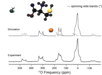
Figure 5.2. Experimental 170 M AS NM R of N-Ac-VL ... 182

Figure 5.3. One-dimensional 5_{N-170 REAPDOR dephasing curves of the leucine (blue,} circle) and valine (red, squares) nitrogens of N-Ac-VL...185

Figure 5.4. Experimental and simulated one-dimensional I3C-170 ZF-TEDOR buildup curves as a function of mixing for (a) leucine carbonyl, (b) valine carbonyl, (c) Ca...189

Figure 5.5. Two-dimensional 13C-170 ZF-TEDOR spectrum...191

Figure 5.6. MAS NMR of N-Ac-VL (a) 'H direct detection (Hahn echo), (b) one-dimensional 'H-170 R3_{-R-INEPT and (c) two-dimensional 'H-170 R}3_{-R-INEPT spectrum...192}

Figure 5.S1. MALDI mass spectra of 170 labeled FMOC-L-leucine and FMOC-L-valine ... 194

Figure 5.S2. 13C{1H} CPMAS spectra of FMOC-L-leucine (a) and FMOC-L-valine (b) ... 194

Figure 5.S3. 17 experimental (solid) and simulated (dashed) MAS NMR spectra of FMOC-L-leucine (right) and FM O C-L-valine (left)...195

Figure 5.S4. 17O experimental (solid) and simulated (dashed) nonspinning NMR spectra of FM OC-L-leucine (a) and FM OC-L-valine (b)...196

Figure 5.S5. 170 MAS NMR of N-Ac-VL MAS NMR (a), simulation of MAS NMR spectrum (b) at 17.6 T ( OH/27t = 750 M H z)...196

(13)

(a) and N -A c-V L (b) at 18.1 T ... 197

Figure 5.S7. 3C, 15N, and 'H MAS NMR of N-Ac-VL at 21.1 T ... 198

Figure 5.S8. 2D 1C-"C RFDR with 1.6 ms mixing at 11.7 T ... 199

Figure 5.S9. 2D 13C- 5N ZF-TEDOR with 2.0 ms mixing at 11.7 T ... 200

Figure 5.S10. Comparison of ID 15_{N CPMAS (a) and} 15N-170 ZF-TEDOR with 7.88 ms of m ix in g (b ) at 17 .6 T ... 2 00 Figure 5.S11. Experimental and simulated, including 0.15 A errors, ID 13_C-17_{0 ZF-TEDOR} b u ildup cu rv es ... 2 0 1 Figure 5.S12. Two-dimensional 'H-170 R3_{-R-INEPT spectrum ...} ₂₀₂

Figure 6.1. 699 MHz/460 GHz DNP-enhanced 13C{1H} CPMAS NMR spectra ... 213

Figure 6.2. Overlay of two-dimensional 13_C- 3_{C correlation spectra of AS-SOD...214}

Figure 6.3. 1 3_{C{I H} CPMAS DNP NMR of biosilica encapsulated lysozyme ... 215}

Figure 6.S1. Kinetics curves of free catMMP12 (red) and immobilized catMMP12 (black) ... 217

Figure 6.S2. 5 T DNP enhanced 13C{IH} CPMAS NMR spectra...220

Figure 6.S3. Comparison of 13C{ H} cross-polarization spectra of AS-SOD...222

Figure 6.S4. SEM micrographs of the biosilica composite of catMMP12 (left) and AS-SOD (rig h t) ... 2 2 3 Figure 6.S5. Overlay of 2D '3_C-'3_{C of catM M P12 ...} ₂₂₃

(14)

List of Tables

Table 2.1. 170 Solid State Nuclear Magnetic Resonance Acquisition Parameters...52 Table 2.2. Experimental 170 NMR Parameters for Crystalline Amino Acid Monohydrates ... 61 Table 2.3. Quantum Chemical Calculations (GIPAW) of 170 NMR Parameters for Crystalline

A m ino A cid M onohydrates... 62 Table 2.S1. "0 GIPAW Calculated Parameters for Neutron and X-ray Structures using

H-optim ized Structures... 88 Table 2.S2. Crystalline and GIPAW-optimized Structural Data for Crystalline Amino Acid

M onohy drates ... 90 Table 2.S3. Summary of X-ray and Neutron Diffraction Data for Crystalline Amino Acid

M on ohy drates ... 9 1 Table 3.1. Experimental 170 NMR Parameters for the Water in Ba(C1O3)2 H20 at 300, 170,

an d 10 5 K ... 10 7 Table 3.S1. Structural Details and GIPAW Calculated 170 EFG Parameters for

B a(C l0 3)2 H 20 ... 12 6

Table 3.S2. GIPAW Calculated 170 EFG Parameters for Ba(Cl03)2 H20...126

Table 4.1. 170 EFG and CSA Tensor Parameters Determined from MAS and MQMAS NMR. 145 Table 4.2. "N CSA Tensor Parameters Determined from MAS NMR...150 Table 4.S1. 2_{H Spin-Lattice Relaxation Values (Ti) LMN.24D}

20 - 1% Gd...160

Table 5.1. Amino Acid and Dipeptide 170 NMR Parameters...180

Table 5.2. O-C/N/H Intra- and Inter-molecular Distances of Interest Within N-Ac-VL ... 188 Table 6.S1. DNP 'H Enhancements (F) and 1H Polarization Build-up Time Constants (TB) at

Different Fields for Enzymes Entrapped within Biosilica Containing 10 mM T O T A P O L ... 22 1

(15)

Chapter 1: Introduction

1.1. General Theory of Nuclear Magnetic Resonance

Since its inception in 1946,1-2 nuclear magnetic resonance (NMR) spectroscopy has been a powerful tool used to elucidate structure and characteristics of chemical systems in both the liquid and solid state in chemistry, biology, and materials science. NMR is at its core the measurement of nuclear spin transitions of NMR active nuclei, which possess non-zero spin angular momentum that is represented by the spin quantum number I (e.g., I= 1/2, 1, 3/2, 5/2,

etc.). In this chapter the basics of NMR relevant for subsequent chapters of this thesis will be discussed in the framework of single spin transitions. Detailed descriptions of the quantum mechanical treatment of NMR theory can be found in a variety of texts. 3-8

1.1.1. The External Interactions

The NMR Hamiltonian is generally described using two categories of interactions, internal and external, so termed due to the origin of the interaction with respect to the nucleus. The external interactions, Zeeman and radio frequency, are discussed in this section, while the

(16)

internal interactions of interest are discussed in subsequent sections. Each NMR active nucleus can be thought of as a microscopic spinning top with a magnetic dipolar moment, Ft,

i = yI, (1.1)

where I is the spin angular momentum vector of the nucleus, and y is the gyromagnetic ratio. The Zeeman Hamiltonian, which describes an NMR active nucleus in an external static magnetic field is given as

Hz = BO. (1.2)

With the external static magnetic field, BO, along the z-axis the Zeeman Hamiltonian can be written as

Hz = -yhIzBO = -hwoI z, (1.3)

where h is the reduced Planck's constant, Iz is the z component of the spin angular moment vector, and ioO is the Larmor frequency of the nucleus. For each NMR active nucleus there are 21+1 energy levels with 21 transitions between these levels as given by operating the Zeeman Hamiltonian on the spin wavefunctions

HzII,m) = -yhBomII,m), (1.4)

where m is the eigenvalue of the eigenfunction Iz and can have a value of I, 1-1,... -I, with I being the spin quantum number of the nucleus. Therefore, the energy of each eigenstate is given as

EI,m = -yhBom (1.5)

for the spin I= 1/2 case the energies become E1/2, 1/2= 1 yhBO with the difference between

these two energy levels being given by

AE = yhBO = w0h. (1.6)

(17)

m = -1/2

E _yhBO

m =+1/2

B

0= 0

_B

₀

Figure 1.1. Energy diagram for the Zeeman interaction for a spin I = 1/2. The energy difference between the two energy eigenstates is given as yhBO

The population difference between these two energy levels is given by the Boltzmann distribution. This net polarization difference is quite small and can be expressed as

P = yhBO (1.7)

2kBT

where kB is the Boltzmann constant, and T is the temperature. Therefore, the polarization of the NMR experiment is linearly dependent on the magnitude of the external magnetic field. The polarization will be aligned along the z-axis; however, to detect the NMR signal, the magnetization must be in the xy-plane. This is achieved by applying a second, but much smaller, external magnetic field, BI, in the form of a radio frequency (RF) pulse orthogonal to the static external magnetic field. The applied B1 oscillates at, or near, the Larmor frequency and thus

effectively tilts the overall magnetic field, or effective magnetic field, away from the z-axis and into the xy-plane, as shown in Figure 1.2. The precession in the xy-plane then induces an EMF signal in the NMR coil according to Faraday's Law; this process is known as magnetic resonance. The RF Hamiltonian is given by

(18)

where (ORF is the frequency of the applied RF pulse used to generate the oscillating B, magnetic

field.

(a) z (b) z (C) (d) Z

net B - magnetic B B Bff B

magnetization field 0 eff

vector vector

By 1

X"OI X X W X

Figure 1.2. Vector representation of magnetic resonance. The alignment of the net magnetization vector (a) is tilted from the z-axis into the xy-plane via a B1 field applied along the y-axis that oscillates at the same frequency as the

precession about the z-axis (b-c). The resulting magnetic resonance (d), where the alternating small magnetic fields (b-c) have shifted the net magnetization vector from the z-axis into the xy-plane.

1.1.2. Magic-Angle Spinning

Unlike solution NMR spectroscopy, where molecular tumbling averages the anisotropic contributions for each NMR interaction, solid-state NMR is generally performed in samples that include many different crystallite orientations that contribute to broad resonances in the NMR spectra. Therefore, in solid-state NMR to achieve high resolution spectra, the sample is reoriented by fast sample spinning about a single axis, OR, with respect to the direction of the external magnetic field, as shown in Figure 1.3(a). The fast sample spinning exploits the spatial dependence of the anisotropic NMR interactions that are defined for second, D, and fourth, G, rank interactions as

D = DO(6R) + D1(OR,OR)+ RD 2 (OR, R), (1.9)

(19)

where the n = 0 (DO, GO) components are only dependent on the sample spinning axis with respect to the external magnetic field and can be eliminated when the angle, OR, is set to the roots

of the second or fourth rank Legendre polynomials

P2(cos 0) oc (3 cos2 OR -1), (1.11)

' ₄(cos 0) oc (35 cos4 _{OR -30 cos}2 _OR+3). _(1.12)

The root for the second-order Legendre polynomial yields a sample spinning angle of 54.736' to eliminate second-order anisotropic NMR interactions. The magic-angle spinning (MAS) experiment, as it is termed, is when the fast sample spinning axis is set to this particular angle, which causes the anisotropic contributions to most NMR interactions to average to zero, as shown in Figure 1.3(b). There are two roots to the fourth rank Legendre polynomial, 30.556' and 70.124 , which eliminate the n = 0 term in the case of fourth rank anisotropic contributions to the NMR interactions. Note that there is no common root to the second and fourth rank Legendre polynomials and therefore second and fourth rank anisotropies cannot be eliminated simply by spinning the sample about a single axis; this topic will be further discussed in Section 1.1.5.1.

Despite the fact that the large n = 0 term in the spatial dependence of the anisotropic interactions is eliminated by spinning about the angle OR, the n # 0 terms are not solely

dependent on this angle but are also dependent on the angle of reorientation of the sample, <R (ORt, which causes these terms to be modulated at the frequency noR and are only found to be zero at integer multiples of 22t/n(oR. These terms are responsible for rotary echoes in the NMR experiment that manifest as spinning sidebands in the MAS NMR spectra, as shown in Figure 1.3(b).

(20)

(a)(b

(A)i

Bstationary

+

- 4-Al

LLUL

A A1.08

kHz,

R I

I

3.0 kHz 6.3 kHz 550 450 350 250 150 15_{N chemical shift (ppm)}

Figure 1.3. Visualization of the MAS rotor spinning at the magic angle with respect to the external magnetic field

(a). Simulation of stationary spectrum and experimental MAS spectra (b) of 5N of nitrate groups in LMN (see

Chapter 4 for more details) at various spinning frequencies demonstrating the spinning sideband patterns of the chemical shift anisotropy.

1.1.3. The Chemical Shift Interaction

Each NMR active nucleus has a unique local environment that will interact with the external magnetic field, BO, to enhance or diminish the strength of the magnetic field at the nucleus. The difference in the strength of the external magnetic field at the nucleus due to the shielding of the external magnetic field by the local nuclear environment is known as the nuclear shielding interaction. The nuclear shielding interaction Hamiltonian is

Ha = yhI e o BO, (1.13)

where a is the second rank nuclear shielding tensor. The nuclear shielding of a bare nucleus is given as a = 0, and therefore increasing nuclear shielding corresponds to an increase in the

(21)

electron density around a nucleus of interest. The particular nuclear shielding of each nucleus produces a slightly different precession frequency

w

= -y(1 - ajsO)BO (1.14)

where Giso is the isotropic nuclear shielding

uiso

= 1Trtc} = (OZZ + 0YY + oXX), (1.15)

where Uzz, Gyy, and cxx are the eigenvalues of the nuclear shielding tensor, also termed the principal components. However, the magnitude of the nuclear shielding is ~10-6 in comparison to the Zeeman interaction and therefore determining the shielding of a nucleus is difficult. Consequently, the chemical shift interaction, which is defined as the shift of the resonance frequency of a particular nucleus in comparison to a reference nucleus, is utilized to denote different resonance frequencies in NMR. Thus, the chemical shift Hamiltonian is given as

H,5 = yhI 8 a BO, (1.16)

where 6 is the second rank chemical shift tensor, and the isotropic chemical shift is given by

(iso _ 1ref-Oiso _S1 _ Wiso-Wref (1.17)

- -ref _Wref

is = 1 Tr{} =) (6'z + +

s,2),

(1.18)

where, Gref is the nuclear shielding of a reference nucleus, oiso is the isotropic frequency of the

nucleus of interest, and Orer is the frequency of the reference nucleus. Thus, the chemical shift and nuclear shielding have opposite sign and an increase in nuclear shielding results in a decrease in chemical shift. While trends in chemical shift and nuclear shielding are directly relatable, absolute nuclear shielding values cannot be trivially obtained from the chemical shift information available from the typical NMR experiment. An exact nuclear shielding reference compound is required to compare chemical shift values to their nuclear shielding counterparts.

(22)

While the principal components of the chemical shift tensor can be utilized to describe the chemical shift tensor, to describe how the chemical shift tensor affects the NMR spectrum two contributions, the isotropic and the anisotropic, are utilized. The isotropic chemical shift, as defined in Equations 1.17 and 1.18, is the entire isotropic contribution. The anisotropic contribution to the chemical shift tensor has angular dependence that can be exploited to provide structural information regarding the orientation of the chemical shift tensor with respect to the molecular orientation. Molecular tumbling in solution state NMR eliminates this orientation dependence and thus averages the anisotropic contribution of the chemical shift tensor to zero yielding narrow isotropic NMR resonances that are dependent only on the isotropic chemical shift. However, for a solid sample the chemical shift tensor manifests as a powder pattern that can be described using both the isotropic and anisotropic contributions (Figure 1.4).

The anisotropic contribution to the chemical shift tensor is defined using multiple different conventions, two of which will be discussed, Haeberlen9_-1₁_{and Herzfeld-Berger.12} While the Haeberlen convention describes the traceless, i.e., having removed the isotropic contribution, principal components of the chemical shift tensor and therefore is found to be more useful when comparing to the molecular or crystal-axis system, the Herzfeld-Berger convention better describes the experimental NMR lineshape due to the anisotropic contribution of the chemical shift tensor. The Haeberlen convention defines the traceless principal component of the chemical shift tensor as

ISzz - SisoI

ISxx

- SisoI

ISyy

- 5iso . (1.19) Thus defining 6zz as the component that is farthest from the isotropic value and 6

yy as the

(23)

Haeberlen convention to define what is called the chemical shift anisotropy (CSA) tensor are defined as the chemical shift anisotropy, (6, and the chemical shift asymmetry parameter, rj6,

(= Szz -

65so,

(1.20)

8

Syy-6Sxx

r76 = !1 **,(1.21)

where 16 can be a number from 0 to 1, and (6 can be either positive or negative depending on the direction of the anisotropy in the chemical system. The Herzfeld-Berger convention defines the principal component of the chemical shift tensor as

(1 > (52 2 633. (1.22)

The two components using Herzfeld-Berger convention that describe the CSA tensor are the span, Q, and skew, K,

fl = 6 -- (33, (1.23)

K 3(822-6 iso) (1.24)

D

where Q is the full width of the NMR lineshape due to the anisotropic contribution, and K is

indicative of the shape of the anisotropic NMR lineshape and is a number between 1 and -1. The Haeberlen and Herzfeld-Berger conventions are demonstrated for a typical CSA lineshape in Figure 1.4.

(24)

&YY ZZ i'so

X

Haeberlen (a) 5 > 0 22 61 Siso ₆3 Herzfeld-(c) Berger 550 450 350 250 150 1_{N chemical shift (ppm)}

Figure 1.4. Haeberlen (a,b) and Herzfeld-Berger (c) CSA conventions demonstrated on a CSA powder pattern. The Haeberlen convention"' for both Q6 positive (a) and negative (b) demonstrating the switching of the 5xx and 6zz components. The Herzfeld-Berger convention'2 showing the span of the CSA pattern and the three principal

components of the CSA tensor.

1.1.4. The Dipolar and Scalar Interactions

1.1.4.1. The Dipolar Interaction

The magnetic fields of NMR active nuclei in proximity to one another interact causing modifications to the total magnetic field experienced by each nucleus. This through-space interaction is known as the nuclear dipole-dipole interaction,

(25)

D 'to1h2 2

D 2y1 2 (1 212, (1.25)

where I is the spin quantum vector for each spin, D12 is the dipole interaction tensor, r is the internuclear distance, i is the internuclear unit vector, y, is the gyromanetic ratio of each spin, and pto is the magnetic permeability constant. Utilizing spherical coordinates and the raising and lowering operators the dipolar Hamiltonian takes the form,

HD h2YY2 (A + B + C + D + E + F), (1.26) where

A = IJzI2z(3 cos2 0 - 1), (1.27)

B = - (+II- + I-1+)(3 cos2 _{_}_1), _(1.28)

C = - (I[I22 + IizI4) sin 6 cos Oe-1 , (1.29)

D = - (IjI2z + IizI2) sin6 cos

6e 'P,

(1.30)

E = - I+j sin2 _{0 e-2i'} _(1.31)

F = - 3II2 sin2 0 e 2 +, (1.32)

where 0 is the angle between the internuclear vector and the external magnetic field. While, the A and B terms will produce a significant effect on the energies of the NMR eigenstates; the C through F terms will produce a small effect on the correction to the energies of the eigenstates according to perturbation theory and are generally ignored in the zero order approximation.''3

Therefore, the homonuclear dipolar coupling Hamiltonian becomes

$D,homo = - h hzY₁Y2 (3I12zz - I1 * 12)(3 cos2 0 - 1). (1.33)

The heteronuclear dipolar coupling Hamiltonian is given as

HOlletero = - 4 hzy1y2 21z1Z(3 cos

2

(26)

due to the truncation of the B term. The dipolar coupling constant between two NMR active nuclei,

D = b12 =

/-'0

h2Y1Y2 (3 cos 2 6- 1), (1.35)

is used to denote the magnitude of the dipolar coupling interaction between two spins. The relation of the dipolar coupling constant to the internuclear distance can be exploited to provide structural constraints of the chemical system being studied.

However, due to the spatial dependence of the nuclear dipole-dipole interaction to the external magnetic field the use of MAS NMR causes an averaging of the effect of the dipolar coupling and reduces the structural information that is available from the MAS NMR experiment. The attenuation of the dipolar coupling depends on the magnitude of the dipolar coupling with the MAS spinning frequency required to be several times larger than the magnitude of the dipolar coupling for the effect to be entirely attenuated. When nuclei are in close proximity, such as 'H-'H homonuclear (D > 50 kHz) and 'H-1 3_{C heteronuclear (D > 15 kHz) interactions,} traditional MAS (COR/ 27t < 30 kHz) fails to fully attenuate the dipolar interaction and the use of

RF decoupling is required to reduce the broadening of the NMR resonance due to the dipolar coupling. Decoupling is typically performed by RF irradiation of one of the nuclei via either continuous-wave or multiple pulse irradiation.4' 7-8, 14-15 This causes the spin Hamiltonian to be

disrupted by rapid spin transitions that occur at a rate larger than the interaction that is being decoupled, therefore causing the Hamiltonian to be averaged to zero.

While resolution is gained using MAS and decoupling to obtain purely isotropic spectra, the structural information in the dipolar coupling is sacrificed. The reintroduction of the dipolar coupling can be achieved by applying a chain of RF pulses that are rotor synchronized at specific times during the rotor period or by RF irradiation that takes advantage of the mechanical motion

(27)

of the rotor that will cause certain terms of the dipolar Hamiltonian to be reintroduced and thus allows the r-3 dependence of these terms to be measured. Common homonuclear and heteronuclear recoupling experiments include, rotary resonance recoupling (R3

),16 radio-frequency driven recoupling (RFDR),17 rotational-echo double resonance (REDOR),'" and transferred-echo double resonance (TEDOR).19

In the R3 experiment, the dipolar coupling is reinstated by RF irradiation at a nutation frequency that is an integer multiple of the rotor frequency (yB,/2t = ncOR/2r where n = 1, 2, etc.). In the case of REDOR and TEDOR recoupling, 7r-pulses, designed to invert the magnetization, are applied twice per rotor period causing the spatial and spin components of the dipolar Hamiltonian to change sign twice in each rotor period causing the net dipolar coupling Hamiltonian to be nonzero. This allows the dipolar coupling to be measured in the REDOR and TEDOR experiments and permit interatomic distance to be extracted due to the r-3 dependence of the dipolar coupling.

1.1.4.2. The Scalar Interaction

The electrons of two covalently bonded spins will couple to the spin states of the nuclei. The interaction of these directly bonded nuclei is termed the J-coupling, or indirect spin-spin coupling,

Hj = h[I1

0

J12 * 12], (1.36)

where J12 is the J-coupling tensor. Due to the small size of the J-coupling, ~ tens of Hz, in comparison to the dipolar coupling and the chemical shift interactions, the J-coupling is generally not utilized in solid-state NMR experiments.

(28)

1.1.5. The Quadrupolar Interaction

More than half of NMR active nuclei have I > 1/2, (e.g., 2_H, ₁4_N, _170,2 3_{Na, etc.) and} therefore possess a non-zero electric quadrupole moment. NMR active nuclei with spin I> 1/2 are called quadrupolar nuclei. The electric quadrupole moment produces a non-symmetric nuclear charge distribution (Figure 1.5) that interacts with the electric field gradient (V) to produce the quadrupolar interaction. The quadrupolar interaction Hamiltonian is given as

HI = _Q Q" IO.VO.I , (1.37)

21(21-1)h

where e is the elementary positive charge, I is the nuclear spin, V is the Cartesian electric field gradient (EFG) tensor, and

Q1

is a constant that describes the nuclear electric quadrupole moment. The electric field gradient contains information about the electric charge distribution

near the quadrupolar nucleus that is related to the local structural environment of the nucleus.

(a) (b) v p BO

,vy

vxx/

0

Figure 1.5. Diagram demonstrating the nuclear charge distribution of the magnetic dipole moment (a) and the

electric quadrupole moment (b). The magnetic dipole moment, p, causes precession about an external magnetic field (a). The electric quadrupole moment, Q, causes the nucleus to precess in an electric field gradient (shown as + and

(29)

The quadrupolar interaction is better understood when presented in a different form than that in Equation 1.37; employing irreducible spherical tensor components6, 9, 20 the quadrupole Hamiltonian can be written as

H =~ 2(2 m(-l)m R2,-T2,m(I), (1.38)

where R2,-.m is the spherical EFG tensor, T2,m is the spin tensor that governs the evolution of the

spin dynamics. The elements of the R2,-m spherical tensor relate to the Cartesian EFG tensor by

R2,0 = jzz, (1.39)

R2,+1 = TEzx i vzyl, (1.40)

R2,+2 = 1 [Vx-~ Vyy 2iVxyJ, (1.41)

where Vap are the components of the Cartesian EFG tensor. The quadrupolar coupling constant, CQ and asymmetry parameter, io, are used to describe the EFG tensor and are defined as

C = e Qyivzz (1.42)

77Q = v"" _vzz ". (1.42)

The quadrupolar interaction Hamiltonian can be rewritten in the form

HQ = -Ym(-l)m R2,-mT2,m(I) (1.43)

where (oQ is the quadrupolar frequency and is defined as

67rCQ

(.4

UOQ = 21(21-) (1.44)

The quadrupolar interaction can be pictured as successive perturbations to the overall Hamiltonian (which is dominated by the Zeeman interaction) and as such we can evaluate the quadrupole Hamiltonian using perturbation theory. The corrections to the energy levels of the

(30)

NMR Hamiltonian due to the quadrupolar interaction are shown for a spin I= 5/2 nucleus in Figure 1.6.

B =0 ₀ H _z + H _Q + H()_Q

Figure 1.6. The energy level diagram for a spin 1= 5/2 nuclei for the Zeeman interaction with the first and

second-order correction of the quadrupolar interaction. The central transition is indicated on the full Zeeman+quadrupolar

interaction levels.

The first order correction to the quadrupolar interaction Hamiltonian,

Hl

R2,0 L 0)(iIT2,0(I|0)(i= R-2,OT2,0(I), (.5

can be described by the correction to the quadrupolar transition frequency arising for a transition between the energy levels i and j as

flil (0, mi, mi) = COQ [IDIQ)(0) 0 d, (Mi, mj)], (1.46)

where

IDIQI(O) = R2,O(E), (1.47)

3 Vzz

and

d(mi,

)

, T2 ) M) - (I, mi T2,O(I)|I, mi)

Mi ~ ~ ~ ____ (I -i1'()1 3

(31)

mi and mj are the initial and final eigenvalues of the energy levels of the transition. As discussed in Section 1.1.2 the DIUM(O) component contains the second-rank Legendre polynomial and therefore the anisotropy of the first-order quadrupolar correction is averaged under fast sample

spinning at the magic angle.

The second-order correction to the Hamiltonian,

-(2) h> R2,-mR2,mT2,m(I)T2,m(I)

QQ 9Vz7 m

can be expressed in the rotating tilted frame, analogous to magic-angle spinning, as R(2= ) 0 ,2,4 ha,0 =1 P,2)TO (I), (1.50)

QQ 9V2QIL=O,,3Z, E=1,3 7TL,J 1,0(I

where 7T2,2 are coefficients that depend only on I in the J=1 terms and are constants for J=3.6

The second-order correction to the quadrupolar transition frequency is given by

,Q (E), -mi, mj) = [s . cO(Mi, m)] + ' [DQQ)() - ( + _ [GQQ)(O)

-C4 (Mi, M), (1.51)

where SM{Q1 contains no angular dependence and therefore contains only isotropic contributions to the second-order correction to the quadrupolar transition frequency, JtQQ(O) is the same spatial component from the first-order correction and is averaged by MAS, and GQQ)(E0)) contains the fourth-rank Legendre polynomial and is therefore this contribution to the second-order correction contains anisotropies that are not averaged by MAS. The cL(mi, m) terms are the spin transition terms and are defined as

(32)

1.1.5.1. MAS and the Quadrupolar Interaction

The spatial dependence on zero-, second-, and fourth-rank Legendre polynomials of the second-order quadrupolar interaction causes the failure of the MAS experiment to produce purely isotropic spectra. The term in the second-order quadrupolar frequency contribution that lacks an angular dependence gives rise to an isotropic contribution to the NMR resonance frequency. The addition of this isotropic quadrupolar frequency prohibits obtaining spectra of quadrupolar nuclei that have a frequency axis that is chemical shift, unless in the limit that 'oQ

«

oo. The term that contains dependence on the second-rank Legendre polynomial will be averaged by the MAS experiment; however, the term that has a spatial dependence on the fourth-rank Legendre polynomial will not be averaged and will cause residual line broadening in the MAS experiment. The residual second-order quadrupolar broadening is typically on the order of a few to tens of kilohertz, as shown in Figure 1.7. While the broadening is rich in structural information due to its dependence on the EFG environment about the nucleus, the broadening of the resonances diminishes the ability to obtain high-resolution NMR spectra via the basic MAS experiment.

(33)

(a) (b) B0 I I I I I I I I 200 0 -200 100 0 -100 170 Frequency (ppm) ₁₇₀Frequency (ppm) (c) (d) 00 44-54.74* 100 0 -100

70.12*

10 Frequency (ppm) -0.5 30.560

Figure 1.7. Simulated '70 NMR spectra for Ba(C103)2-H21 70: stationary (a), fast sample spinning about 54.736' (b), and fast sample spinning about 70.124' (c) demonstrating the broad lineshapes associated with MAS and quadrupolar nuclei. The second- and fourth-rank Legendre polynomials showing the roots where interactions with these spatial symmetries are averaged (d).

1.2. Introduction to

170

NMR in Biological Solids

Oxygen is vital to the structure and function of biomolecular systems as one of the fundamental building blocks of biomolecules and through its role in hydrogen bonding. 1-22

However 170, the only NMR active oxygen nucleus, has yet to be exploited as a consistent tool in solid-state NMR studies of biomolecular solids; while other spin I = 1/2 nuclei, such as, 'H, "C, "N, and 31_{P, have long been routine probes of the structure and function of biological}

systems via solid-state NMR. 2-27 Oxygen- 17 suffers from several complications that limit its use

in structural studies of biomolecular solids: 170 is a quadrupolar nucleus (I = 5/2) with a low natural isotopic abundance (~0.037%) and a low gyromagnetic ratio (Y170 = -5.8 MHz/T;

(34)

yields broad resonances on the order of kilohertz (~5-8 kilohertz at 21.1 T in biological solids). Despite these difficulties, the chemical shift dispersion of 17 for biologically relevant

environments has been found to be ~400 ppm, a two-fold increase in comparison to 13C,1

3

, 28-32

thus indicating the appeal of 170 NMR as a probe of structure and function in biomolecular

systems.

While "0 has not become a reliable probe in biologically related solids, 170 studies have been performed on biological solids taking advantage of isotopic enrichment, population transfer techniques, and high magnetic fields.28

-29

, 31-48 The use of quantum chemical calculations to

supplement 170 NMR results in biological solids has been shown to assist in examining the

effect of various 170 related interatomic distances and angles on the quadrupolar coupling

environment.4_6-49 _{One such study probed the structure of nucleic acid bases with regard to the}

hydrogen bonding environment and its effect on the EFG tensor parameters.40 With increased magnetic fields available for 70 NMR studies in biological solids, dipolar recoupling

techniques, such as REAPDOR,50 TRAPDOR," and S-RESPDOR,2 have been deployed to measure interatomic distances involving 170 in biomolecular solids.35

, 53 While these studies are promising they have relied on one-dimensional experiments that lack the resolution necessary to be employed for complex and fully labeled systems and have thus been limited to systems that

are selectively labeled.35, 53

Despite the promising gains in isotopic enrichment and magnetic fields in recent years, the lack of resolution resulting from 170 MAS NMR experiments precludes the ability to

examine complex biological solids.29, 31, 48, 54-58 Therefore, to increase the resolution of 170 MAS

NMR experiments the second-order quadrupolar broadening must be eliminated; this can be

(35)

'61-62 multiple quantum MAS (MQMAS), - or satellite-transition MAS (STMAS).69 70 While the

first two of these techniques average the second-order quadrupolar broadening via special instrumentation, the latter two utilize spectroscopic means using traditional solid-state NMR hardware. The MQMAS experiment is the most commonly utilized to produce purely isotropic

170 _{NMR spectra due to its ease of implementation; however, the excitation efficiency of}

MQMAS is diminished for the quadrupolar couplings that are present in biological solids.3 3,45

,66-67

To further combat the limited signal-to-noise of 170 NMR in biological solids, dynamic

nuclear polarization (DNP) has been performed to enhance the sensitivity of 170 .71-77 The addition of DNP to the traditional stable of "7 MAS NMR experiments on biological solids will allow experiments to be performed that would have previously been ineffective.

1.3. Introduction to Dynamic Nuclear Polarization

Increasing the signal-to-noise of the NMR experiment is a fundamental aim of NMR experiment design and hardware development. The primary source of increased signal-to-noise in NMR is by increasing the polarization, which can be achieved in three ways: increasing the external magnetic field, decreasing the temperature of the experiment, and transferring polarization from a more sensitive spin to a less sensitive spin. The first of these has yielded external magnetic fields in excess of 21.1 T (OOH/ 2n = 900 MHz); however, the expense to

develop and produce magnetic fields of this magnitude precludes wide availability of these instruments. While decreasing the temperature can yield a nearly four-fold increase in the polarization using liquid nitrogen (-77 K), the increase in signal-to-noise is limited by the expense and difficulty in decreasing the temperature further. The transfer of polarization by the

(36)

traditional cross polarization that exploits the high sensitivity of the 'H nucleus to enhance the polarization of lower sensitivity nuclei has become routine in solid-state NMR.78 _{However, the}

polarization enhancement that is available in the cross polarization experiment is limited by the increase in gyromagnetic ratio between 1H and the detection nucleus to approximately one order of magnitude or less. To increase the polarization enhancement further, dynamic nuclear polarization can yield gains in sensitivity of multiple orders of magnitude (~660 maximum theoretical enhancement for 'H) by transferring polarization from an electron to a nucleus of

interest.74' 79-86

While DNP was first proposed in 1953 by Overhauser,83 _{high-field DNP NMR (> 5 T)}

was limited due to a lack of high frequency (> 140 GHz) microwave sources with sufficient power (> 3 W) to facilitate the necessary electron-nuclear transfer. With the advent of high frequency high power gyrotrons,79 high field DNP NMR has provided significant gains in sensitivity demonstrating the ability to study new and interesting chemical systems.74-77, 82, 87-89 The typical DNP NMR experiment is performed by transferring electron polarization to 'Hs within the NMR sample by irradiating the sample with high power microwaves. The polarization is then transferred to other nuclei of interest via cross polarization, termed indirect polarization (e~-'H-X). Both indirect and direct polarization (e--X) have been shown to be effective methods for DNP.79_'_81,87-110_{To increase the effectiveness of the DNP NMR experiment the temperature is}

decreased to < 100 K to lengthen the electron and nuclear spin-lattice relaxation times and better facilitate the electron-nuclear polarization transfer.

The solid and cross effect are the two most commonly used solid-state DNP mechanisms in insulating solids. The solid effect (SE) is a two spin process that is the dominant DNP mechanism when the homogeneous (6) and inhomogeneous (A) electron paramagnetic resonance

(37)

(EPR) linewidths are less than the nuclear Larmor frequency (ool), ooI > 6,A.86' 111-114 The

transitions present in the SE are formally forbidden but become partially allowed due to the mixing of the nuclear spin states caused by the electron-nuclear dipole coupling. When the microwave irradiation is applied at the electron-nuclear zero- or double-quantum frequency, o,

= (oos + coo, as shown in Figure 1.8, the electron polarization is transferred to the nuclear

polarization.

(a) (b) > (C)n

+>~LI.

I

>+

Equilibrium Positive E (DQ) Negative E (ZQ)

Figure 1.8. Energy level diagram for a two-spin (one electron and one nucleus) system, |ms, m), at thermal

equilibrium in a magnetic field (a). The SE conditions for the positive, wos - wo0 (b), and negative, oos + wo0 (c)

enhancements. The green circles are a representation of the spin populations of each spin state (not to scale) to demonstrate the enhancement of the nuclear transitions.

The cross effect (CE) is a three-spin process that occurs between two electrons and a nucleus and is the dominant DNP mechanism when the inhomogeneous breadth of the EPR spectrum is larger than the nuclear Larmor frequency, which is in turn larger than the homogeneous breadth of the EPR spectrum, A > oo > 6.82, 115-119 The condition for CE transitions

arises when the difference between the Larmor frequencies of the electron spins are approximately the nuclear Larmor frequency, 00 - oosi - OOs21, as shown in Figure 1.9. When

microwave irradiation is applied at either electron transition, the degenerate matching condition induces a process that can cause a large polarization transfer from the electrons to the nucleus.

(38)

biradicals8 5

, 120 to minimize the electron concentration over the use of monoradicals. The

enhancement that is present in biradical polarization agents is determined by multiple factors, including molecular orientation, the electron relaxation rates, the solubility, and the internal Hamiltonian of the electron spin. Detailed descriptions of the solid and cross effect DNP mechanisms can be found elsewhere.82' 84-86, 115, 121

(a) (b) (c) I01 1++

=-a-W

1+-+i>

1+-->

e---Equilibrium 1+ + +>E 3 A

Posiive>

1+-+ 1++ > I- --> 1- -+

ALM.

0 0 C,, 00

Negative

E

Figure 1.9. Energy level diagram for a three-spin (two electron and one nucleus) system, ins₁, MS2, mi), at thermal

equilibrium in a magnetic field (a). The CE conditions for the positive (b) and negative (c) enhancements. The microwave irradiation saturates the electron transitions and the degeneracy of the middle levels leads to a saturation across WCE that yields enhanced nuclear transitions. The green circles are a representation of the spin populations of

each spin state (not to scale) to demonstrate the enhancement of the nuclear transitions.

1.4. Overview of Thesis

The characteristic chemical shift of 170 in water bound to amino acids and dipeptides is

studied in Chapter 2, demonstrating the unique chemical shift range for 170 of bound water in

Advances in oxygen-17 NMR for biological structure determination

JUL

0O6 2017

LIBRARIES

ARCHIVES

Signature redacted

Signature redacted

Signature redacted

Signature redacted

...

Signature redacted

Signature redacted

Table of Contents

List of Figures

List of Tables

Chapter 1: Introduction

1.1. General Theory of Nuclear Magnetic Resonance

1.1.1. The External Interactions

B

B

1.1.2. Magic-Angle Spinning

(A)i

Bstationary

+

- 4-Al

LLUL

A A1.08

I

1.1.3. The Chemical Shift Interaction

w

uiso

s,2),

ISxx

ISyy

65so,

X

1.1.4. The Dipolar and Scalar Interactions

6e 'P,

/-'0

0

1.1.5. The Quadrupolar Interaction

Q1

,vy

0

Hl

)

«

70.12*

1.2. Introduction to

NMR in Biological Solids

1.3. Introduction to Dynamic Nuclear Polarization

+>~LI.

I

I

>+

=-a-W

1+-->

Posiive>

ALM.

Negative

E

1.4. Overview of Thesis

_B