Agglomeration economics, trade, and a system of cities : a general equilibrium approach

A GENERAL EQUILIBRIUM APPROACH

by

YOUNG GAK KWON

B.S., M.C.P., Seoul National University (1970, 1975)

M.R.P., Syracuse University (1978)

Submitted to the Department of Urban Studies and Planning in Partial Fulfillment of the Requirements for the Degree of

Doctor of Philosophy at the

Massachusetts Institute of Technology September 1987

) Young Gak Kwon, 1987

Signature of Author

Department of Urban Studies and Planning September 1987 Certified by -Alan Strout Thesis Co-supervisor Certified by William Wheaton Thesis Co-supervisor Accepted by Langley Keyes Chairman, Department Committee

I would like to express my appreciation to the members of my committee, professors Karen Polenske, Alan Strout, and Bill Wheaton for their time, insights, and comments during the preparation of this dissertation. Alan Strout has kept the faith in me and provided

encouragement in most difficult times. Bill Wheaton's substantive inputs during our thoughtful discussions have been indispensable for this dissertation. During my long stay at MIT, Karen Polenske has always been generous in offering valuable suggestions and guidance. I owe many intellectual debts to them.

AGGLOMERATION ECONOMIES, TRADE, AND A SYSTEM OF CITIES: A GENERAL EQUILIBRIUM APPROACH

by

YOUNG GAK KWON

Submitted to the Department of Urban Studies and Planning in Partial Fulfillments of the Requirements for the Degree of

Doctor of Philosophy

ABSTRACT

A general equilibrium approach that integrates the conventional supply- and demand-oriented approaches to the determination of city size and output is proposed. Among the prominent features of the approach are agglomeration economies and diseconomies, in-dustrial structure of the city, and the interdependence between

cities via migration and trade. The approach is then utilized to relate economic efficiency to alternative city size distributions

in the nation.

The optimum city size distribution in which potential welfare levels of all cities are maximized is attained when all cities become autarkic and of size No, the single-city optimum size. However, under limited facor mobility, a hierarchical city size distribution is more likely to emerge in equilibrium. This

latter city size distribution, though suboptimal, represents mutual benefits for both cities resulting from gains from trade.

Thesis Co-supervisor: Thesis Co-supervisor: Alan Strout, Ph.D., William Wheaton, Ph.D.,

Senior Lecturer in Associate Professor in

CONTENTS

1. INTRODUCTION --- (5)

2. MODELS OF CITY SIZE AND OUTPUT DETERMINATION --- (11)

2-1. Introduction --- (11)

2-2. Demand- and Supply-oriented Models --- (11)

2-3. Localization and Urbanization Economies --- (14)

2-4. Synthesis --- (22) 3. A SINGLE-CITY MODEL --- (26) 3-1. Introduction --- (26) 3-2. Consumer Equilibrium --- (29) 3-3. Producer Equilibrium --- (37) 3-4. Market Equilibrium --- (43)

3-5. Migration and City Size Distribution --- (58)

4. A TRADE MODEL WITH SCALE ECONOMIES --- (66)

4-1. Introduction --- (66)

4-2. Production under "Mild" Scale Economies --- (67)

4-3. A Balanced Free-Trade Model --- (75)

4-4. Migration and Balanced Free-Trade Model --- (98)

5. POLICY IMPLICATIONS --- (115)

6. CONCLUSION --- (122)

LIST OF FIGURES

Fig. 2-1: Hypothetical Economies of Scale with Urban Size -- (20)

Fig. 3-1: Total Labor Supply with City Size --- (36)

Fig. 3-2: Supply and Demand Curves (i=1) --- (48)

Fig. 3-3: Equilibrium Price with City Size (i=1) --- (52)

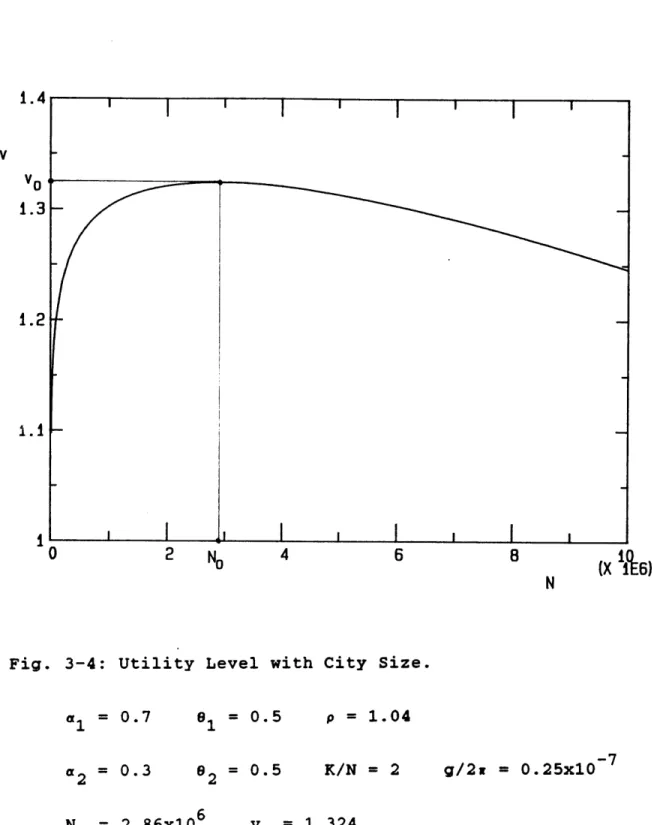
Fig. 3-4: Utility Level with City Size --- (54)

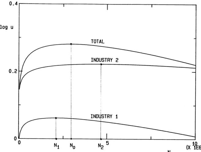
Fig. 3-5: Net Urbanization Economies by Industry (i=1,2) --- (56)

Fig. 3-6: Equilibrium City Sizes (N(2No) --- (61)

Fig. 3-7: Equilibrium City Sizes (N>2N) --- (63)

Fig. 4-1-1: Price Ratio vs. q --- (78)

Fig. 4-1-2: Factor Price Ratio vs. q --- (82)

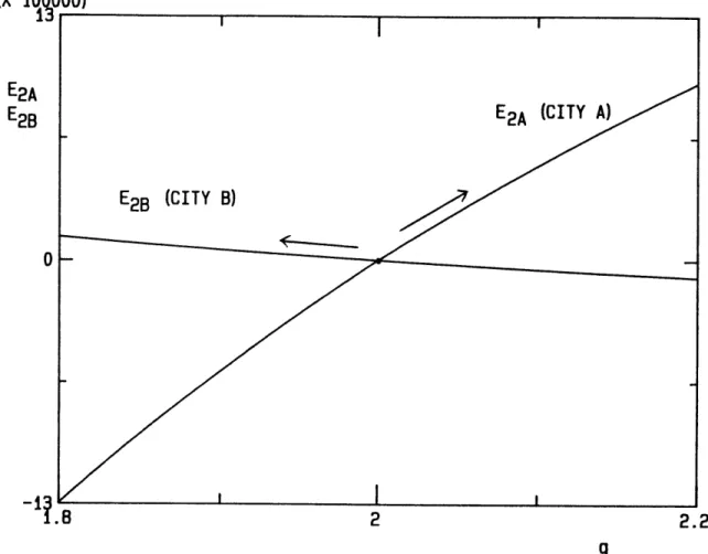
Fig. 4-2: Excess Demand and Supply vs. q --- (86)

Fig. 4-3-1: Numerical Solution of (4.11), p vs. q --- (89)

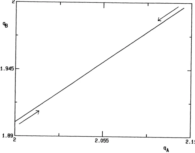
Fig. 4-3-2: Numerical Solution of (4.11), qA vs. qB --- (90)

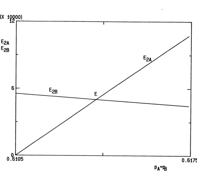
Fig. 4-4-1: Numerical Solution of (4.11) and (4.20), qA vs. E2 --- (92)

Fig. 4-4-2: Numerical Solution of (4.11) and (4.20), p vs. E2 --- (93)

Fig. 4-5: Changes in Utility Levels, Before and After Trade (95) Fig. 4-6-1: Numerical Solution of (4.33), z vs. q --- (103)

Fig. 4-6-2: Numerical Solution of (4.33), z vs. p --- (104)

Fig. 4-7: Numerical Solution of (4.34) --- (106)

Fig. 4-8: Equilibrium Utility Levels vs. City Size Distribution --- (107)

Fig. 4-9: Utility Level with City Size (Single City Model) (110) Fig. 4-10: Population Share of City A vs.

N

Fig. 4-11: Equilibrium Utility Levels vs. National Population --- (112)

LIST OF TABLES

Table 4-1: Solutions to Endogenous Variables

(Trade-Only Model) --- (97) Table 4-2: Solutions to Endogenous Variables

1. INTRODUCTION

With the continuing increase of worldwide urban populations, the importance of cities in regional and national economic

development has become paramount. Thus, many countries now adopt urban policies in order to affect the spatial allocation of

populations among cities as a part of their national economic development planning (Rodwin[1970], Thompson[1972], Reiner and

Parr[1980], Richardson(1981], Renaud[1981]). According to

recent UN reports, eighty-three percent of 114 developing coun-tries indicated that the spatial distribution of their urban population was unacceptable (UN[1978, 1980]). The reports also noted that the reason for such unacceptability was attributed to

a heavy concentration of population in a few large metropolitan centers caused by migrations from small cities and rural areas. These countries seem to believe that unchecked market forces give rise to excessive growth of their largest primate cities, causing unwanted results such as economic inefficiency, regional

in-equality, political unrest, and the familiar "big city headaches" such as congestion, pollution, and overburdened infrastructure and housing.

The emerging concensus among these countries, according to the reports, is that the uneven spatial distribution of popula-tion is the main obstacle to overall socioeconomic development. To the countries, the existence of their largest cities is

practice, therefore, most urban policies have mainly been limited to alleviating the situation in their biggest cities, either to direct more public investments into them or to divert people away from them. Although many countries, such as Brazil, Egypt, and Mexico, have emphasized regional growth and development in small and medium size (or "secondary") cities, such efforts seem to reflect their desire to keep migrants out of large cities, such as Sio Paulo, Cairo, and Mexico City. Rarely has there been a serious commitment to develop the biggest city as well as smaller cities within the context of the national system of cities. What is lacking is the view that the unit of national urban policies must be the national economy rather than the city economy.

Aside from the equality consideration, if spatial urban policies to alter city sizes are needed for national economic development, one has to question the validity of the current

policies on economic efficiency grounds: can the size containment of the largest city enhance the economic welfare of its own

citizens and others in the rest of the country? At least two shortcomings of the current policies can readily be pointed out. First, a preoccupation only with the biggest city and its size merely indicates a greater concern for local development than for national development. By excluding the rest of the country, the current policies may be blamed for their artificially narrow

areal scope. They also seem to lack an explicit consideration of the contribution of the biggest city to the national economy. Second, their focus on the relationship between one city size and

the economic efficiency and welfare within even that city is mis-leading. Unless the city exists in isolation, its size and

efficiency are determined in interaction with the rest of the country. Moreover, a city without being related to the national size distribution of cities may never identify its size measure. In absolute terms, for example, Jakarta may be the biggest city

in its country, but not so by Mexican standards. Of course, no implication regarding the economic efficiency and welfare in Jakarta, let alone its contribution to the national economy, can be drawn from its population size alone. The size and efficiency of a city are a relative concept that can be meaningful only

within the framework of the national system of cities. It is clear that, unless urban policies are directed toward the tional system of cities, they may not be useful in enhancing na-tional economic welfare.

However inadequate the current urban policies may be, they nevertheless seem to reflect the current state of knowledge in

the literature. Although stylized facts such as the rank-size rule and paradigms such as "concentrated decentralization"

(Rodwin[1961], Alonso(19681) exist, it is surprizing that no study has analytically dealt with the basic issue: what spatial allocation of populations among cities is commensurate with na-tional economic development? Ever since Isard raised the ques-tion almost three decades ago, it still remains unanswered

In this dissertation, an attempt will be made to address the issue directly by devising an analytic spatial economic framework in which the economic efficiency and welfare of a city depend not only on its own size and internal characteristics, but also on

those of other cities within the nation. It is hoped that this framework can serve as an analytic basis of national urban

policies in enhancing the overall level of welfare. To this end, we will develop a spatial general equilibrium urban model in

which cities are viewed as centers of production, consumption, and trade. Essential elements of the model will include sizes of cities, industrial composition and production technologies, and economic interactions of cities via migration and trade. With the model, it will then be possible to answer the following related questions. (1) Does an existing size distribution of cities leave room for welfare improvement, and justify a planned intervention? (2) If (1) is so, what would be an alternative size distribution? (3) What would be an available and effective means of planned intervention in a typical mixed economy?

Following the long tradition in the international trade

literature, the model will emphasize comparative statics and will be of a 2 by 2 by 2 (factors, industries, and cities) type, with possible extensions for n-cities where appropriate. In addition to comparative advantage which is the basis of the standard trade model, we will incorporate agglomeration economies into our

model. Thus, it represents an expanded interurban version of the standard international trade model. However, it is well known

that such differences as absence of tariffs and exchange rate concerns, greater factor mobility, similarity in tastes and production technology make the interurban version a unique and more plausible trade model than the international version under

the usual set of assumptions.

In chapter 2, we will review two representative yet polar types of urban models regarding the city's output and size deter-mination. Since both types are incorporated into our model, we will discuss their merits and shortcomings along with the

ra-tionale of our model specification. The single-city model to be developed in chapter 3 will be adapted from discussions made in the previous chapter. It will be the basic tool used throughout this dissertation. We will show how the city's internal produc-tion and consumpproduc-tion characteristics, including its size, deter-mine its welfare level. In chapter 4, we will deal with two cities that are mutually interdependent in the economy by means of balanced trade and exchange of factors. Under different

assumptions, equilibrium sizes and welfare levels of both cities will be determined. We will then examine changes in the equi-librium welfare levels as a result of changes in the size dis-tribution of cities. In chapter 5, we will cover, by utilizing lessons from the previous chapters, some suggestive issues in na-tional urban policies. Due to the scant nature of economic data at the city level in most countries, however, we will rely on numerical analyses rather than on empirical ones. In chapter 6, we will present the conclusions. After a brief summary of the

dissertation, we will delineate limitations of our model and possible directions for future research in urban modelling and policy making.

2. MODELS OF CITY SIZE AND OUTPUT DETERMINATION

2-1. Introduction

Before we build a sound urban model, it is necessary to in-vestigate existing urban models that explain the determination of city size and output. Since the standard assumption is to equate city size with city laborers, most models rely on the mechanics of the urban labor market for explanations. Moreover, since the number of laborers is highly dependent on net migration into a city, urban models put a particular emphasis on the relationship between employment and migration. Two contrasting approaches, each of which emphasizes either the demand or supply side of the labor market, will be reviewed. We will then argue that in-corporation of both views would be necessary to build a spatial general-equilibrium urban model. In addition, refinement of some key concepts for our model specification will be noted.

2-2. Demand- and Supply-oriented Models

Muth[1971], Engle[1974], Schaefer[1977], and Miron[1979] provide a useful classification of urban models on city size and output: the demand- and supply-oriented approach. The former type, which can also be labeled as the external approach,

inherits the Keynesian heritage in urban modelling in that the main emphasis is on exogenous demands from other areas for the output of the city. Factor supplies (labor and capital) are

pre-sumed to be perfectly elastic so that factor in-migrations to the city are limited only by the city's factor demands at given real factor prices. It is further assumed that the demand for

products is price inelastic and that no matter how much is de-manded externally, it will be supplied by the city. Spatially, this implies that the size and output of the city are wholly determined by its output market areas combined with varying

demand intensities over space. Migration becomes the consequence of the city's growth rather than the cause of it. City sizes will be in continuous equilibrium, because migration will always clear the interurban labor market. The familiar export-base model and the various urban hierarchy models, such as

Losch[1954], Beckmann[1958J, and Beckmann and McPherson(1970], belong to this type.

Although there is a consideration in this approach of

mututal interdependence among cities via exports and factor ex-change, and, to a varying degree, of their locations and associ-ated transport costs, it usually does not take account of the city's internal production and consumption characteristics. In Beckmann's model, for example, per capita consumption of a good is held to one unit regardless of its price. With no explicit consideration of comparative costs in production, in particular,

the selection of export sectors becomes rather arbitrary. The level of exports is often exogenously determined, but there is a

complete lack of explanation as to how the level of imports is determined. This approach essentially envisions a hierarchy of

cities based on trade imbalance. Goods are exported only down the hierarchy from large to smaller cities, but there are no corresponding reverse flows. In spite of such criticisms of the demand-oriented approach, it is to its credit that, unlike the supply-oriented approach, establishment of a city size

distribution, albeit unsatisfactory, is feasible within the model.

The supply-oriented, or internal approach, on the other hand, is often concerned with one city in isolation, and repres-ents the tradition in the international trade literature. The main focus of this approach is on the city's production

technol-ogy, endowment of factors, and other internal characteristics. It is often assumed that factor demands are perfectly price elastic, but factor supplies are inelastic due to non-wage considerations. Further, since the city is presumed to face a perfectly elastic export demand at a given output price (or terms of trade), it is suggested that no matter how much the city

produces, it will be purchased elsewhere. This is the familiar "small country approximation" in the international trade litera-ture. Consequently, the output and size of the city are limited only by the internal cost consideration and available factor supplies. Migration now becomes the cause of the city's growth, rather than the response of it. Thus, the city's internal char-acteristics (including non-wage aspects), which presumably are a determinant for potential migrants, become of paramount

In this approach, an exogenous shock, for example, to shift the demand for labor will induce migration into the city, and this will in turn result in an even greater equilibrium city size and output. This "growth-feeds-by-itself" hypothesis has been suggested by many authors including Borts and Stein[1964], Thompson[1968], and Muth(1971]. Although this approach emphasizes the city's various internal characteristics in

production and consumption, its neglect of other cities as both output market and factor supply areas make it highly unrealistic

as a basis of a spatial urban model. In general, due to its lack of the explicit linkage among cities, this approach cannot

establish a distribution of city sizes endogenously. However, since this approach has been influential in the literature and pervasive in the minds of many governments, as it incorporates the concept of agglomeration economies, we will now look into it further.

2-3. Localization and Urbanization Economies

Following the usual Heckscher-Ohlin practice of constant returns to scale production technology, proponents of the pure supply-oriented approach try to find the raison d'Stre of the city in its resource endowment (natural resources included) that gives rise to its comparative advantage. However, the approach

is generally extended to contend that when a city is assumed to be built on homogeneous land, the main economic justification for

the city is the presence of agglomeration economies in production and/or consumption. After Ohlin[1933], Hoover[1937] and

Isard[1956], it is widely accepted that agglomeration economies can be realized at the firm (scale economies), the industry (lo-calization economies), and the city level (urbanization econ-omies) (for example, see Isard[1956]). In the urban context, however, the last two types of agglomeration economies, which are external to the firm, get the most attention. This is because in a city multiple firms of widely different sizes seem to coexist competitively within the same industry. Under the existence of external economies, therefore, firms are usually modelled to operate under constant returns to scale and to behave competi-tively (Kemp[1955,1964], Melvin[1969], Chipman[1970]).

Localization economies, which represent immobile external economies to the firms of each industry, are internal to the in-dustry of the city. They are the result of the enlargement of one industry, which facilitates greater intra-industry

spe-cialization and division of labor in that industry. The enlarge-ment of the industry also means enhanced intra-industry

facili-ties for the firms in terms of collective research, marketing, communication, and innovation. Urbanization economies, which are

external to both the firm and the industry but internal to the city, are the result of greater spatial concentration of all in-dustries and their increased level of economic activities within

the city. These economies reflect all tangible and intangible locational advantages for any firm of any industry in a large and

diverse city economy. Such advantages result from a large city-wide labor market, a well-developed infrastructure, and other

public facilities, which are often lacking in a smaller, less diverse place. _{Thus, the sizes of industries, their composition,}

and inter-industry externalities are all implied to be the com-ponents of urbanization economies of the city. The usual

prac-tice of using the city size alone amounts only to a proxy measure of urbanization economies, however.

Mills[1967] was among the first formally to present an analytic supply-oriented model that incorporates urbanization economies in the production function of a single composite urban good. _{In his monocentric city where firms are located in the} city center surrounded by residential areas, a unique equilibrium size is reached by a sharp increase of commuting costs and con-gestion (urbanization diseconomies) after certain city sizes are attained. The equilibrium city size represents an optimum size at which net urbanization economies (urbanization economies less diseconomies) are maximized. The equilibrium is essentially an autarkic one, and the optimum city size is determined entirely by the internal conditions of the city, regardless of the size dis-tribution of cities in the rest of the country. Because the city is of the aforementioned "one-city-in-isolation" type, and its industrial composition is singular (i.e., city with one aggregate industry), however, the equilibrium city size should mean either of two paradoxical results: there is one city in the country; or all cities are identical. Of course, the naivety of one

universal optimum city size is well known.

An indirect way to sidestep the above dilemma, while staying within the Mills' framework, would be to specify a range of

"efficient" city sizes in which net urbanization economies are positive (Alonso[1971], Richardson[1972]). However, efficiency here refers to neither an optimum nor an equilibrium, and the preoccupation here is to find city sizes for "self-sustaining growth". A more direct solution to avoid the above paradox of one efficient city size, however, is Henderson's recognition that different-sized monocentric cities perform different functions, and they may operate at different, but efficient, equilibrium sizes (Henderson[19741). Each city, producing only one distinct export good, is engaged in free trade with other cities (but not with cities of its own type, the type being determined by the

industry) at exogenously determined terms of trade. Thus, multi-ples of different-sized cities can coexist in equilibrium;

however, cities of the same type must be identical in size.

It should be noted that Henderson's model is established, rather a priori, on complete specialization of cities at all

times in which no distinction can be drawn between the city and the (export) industry (or between urbanization economies and lo-calization economies). The sizes of both are identical when measured by laborers. According to this model, a city, however big it may be, must always be engaged in trade, and unlike the

trade. Henderson notes that complete specialization occurs when there are no prodution benefits or positive externalities from locating two different industries in the same place (i.e., the city center).

If they are located together, because workers in both industries are living and commuting in the

same city, this raises the spatial area of the city and average commuting costs for a given degree of scale economy exploitation in any one

industry. ... Thus, specialized cities will be larger and more efficient than potential non-spe-cialized cities; and they will be able to pay higher factor returns (Henderson (1980], p.17).

However, the statement is premature, and cannot explain even the initial identification of the export sector. Thus, its com-plete specialization is totally unclear. The complete

spe-cialization is rather the result of Henderson's reliance on the so-called small city approximation in which the city produces

(and consumes) on such a small scale that the effect of its production (and consumption) on the national and international markets can be ignored. With no consideration given to other cities as potential market areas, therefore, the complete

spe-cialization is presumed to be feasible. Of course, the identifi-cation and the degree of specialization of the export sector must be determined by production and trade equilibrium conditions, not

a priori. Although complete specialization is always a

possibility, the actual degree of specialization is to be limited by the extent of the market. In light of the fact that the

con-temporary urban concern stems mainly from the alleged gigantism of the largest cities and their pervasive effects on national economies, the small city approximation seems particularly in-appropriate.

Aside from inter-industry production externalities, the possibility of multiple industries in the city is more a rule

than an exception. Later we will show that even under external economies, the production possibility curve of the city is

generally concave. Thus, there exists a rare possibility of com-plete specialization by one industry. This is because, to the extent that the marginal products of factors are finite and dim-inishing even under scale economies, greater specialization by the city in a particular good will eventually increase the marginal (social) opportunity cost of that good. Although the

specific degree of specialization by the city cannot be inferred in the absence of the production functions, even a casual

observation will hold that incomplete specialization is more likely in a large market such as the city. Moreover, as the "home market effect" of the trade literature suggests, it can be argued that the city's size of the internal market determines the range of goods produced, or industrial diversity. Indeed,

industrial diversity or "breadth", to quote Thompson[19681, must be a fundamental characteristic of the city.

It is thus not surprizing to note that the single-industry models of Mills and Henderson generate rather unrealistic

results. _{Quite contrary to Henderson's prediction, for example,} Dixit[1973], in an exercise of such a single-industry model, could not reach an equilibrium city size much in excess of one million, however large the assumed urbanization economies might be. _{Moreover, the existence of a single industry implies that} the output will not respond to a change in price (or the terms of trade). _{Such a rigidity can usually be avoided once multiple} in-dustries are allowed for in the city.

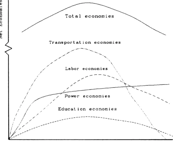
For example, Isard[1956] presents a hypothetical illustra-tion of multiple industries which are subject to urbanizaillustra-tion economies and diseconomies as in Fig. 2-1. It shows four curves for the corresponding representaive industries of the city in which net economies increase first, attain maxima, and finally decrease as city size increases. The top "total economies" curve is meant to represent an overall net economies figure for the city, hopefully after apppropriate weighting of the industry

curves. _{The total economies curve is akin to the single industry} curve implied by the models of Mills and Henderson, but with two different possibilities: outputs can now become price-elastic; and industrial composition can play a role in determination of the equilibrium city size. Thus, the rigidity problem can now be nicely worked out.

Total economies Transportation economies Labor economies Power economies Education economies City Size

Fig. 2-1: Hypothetical Economies of Scale with Urban Size. Source: Isard[1956], p. 187. 0 0 4) rZ / I / / / / 1/

/

--Implicit in depiction of Fig. 2-1 are the usual assumptions of the supply-oriented approach, however. In particular, the curves drawn reflect either the autarkic situation of the hypo-thetical city, or no consideration of other cities in determina-tion of the nadetermina-tional system of cities. It is clear the curves will change readily once the city becomes interdependent with other cities via trade, for example.

2-4. Synthesis

The previous section has shown that the two polar types of urban models attribute city size and output determination mainly to one of two sources: either external demand for the city's output or internal characteristics of the city including agglomeration economies. In view of reality, however, it is abundantly clear that a truly general spatial urban model calls for an integration of both. For the size of the city, its

output, and welfare level are all dependent on those of other cities within the nation.1 In particular, there is a need to in-corporate into our model some refinement of the production

condi-tions typified by the supply-oriented approach, as well as the consideration of demand for the city's output of either internal or external origin indicated by the demand-oriented approach.

1 International trade, an important factor in urban modelling, is beyond the scope of this study.

The single-industry, single-city models of Mills and Henderson nevertheless represent an improvement over the pure supply-oriented models in that they incorporate both urbanization economies and diseconomies albeit in less than satisfactory ways. However, their failure to allow for industrial diversity within

the city seems to generate inconsistencies as noted above. It should also be noted that unless the industrial composition of

the city is known, no efficiency implication can be drawn by the city size alone. This suggests that at least two industries must be introduced to allow for a meaningful industrial composition

and the consequent agglomeration economies realized within the city.

Once the existence of, say, two industries is accepted, there remains the problem of specifying urbanization and lo-calization economies within the model. Despite deliberations made by Hoover and Isard, however, the relationship between the

two agglomeration economies that are external to the firm does not seem well established. As Isard aptly notes, "only a fine line of distinction" separates them. Although their conceptual differences have already been noted, their separate specifi-cations within the model seem to be an intractable problem.

Further work in this area is badly needed. Consequently, we will handle this problem by the following simplified, but reasonable, set of assumptions.

labor market from which labor is allocated between the two in-dustries. The size increase of the labor market along with its greater spatial concentration would enhance its efficiency and allow for a greater potential realization of localization econ-omies for both industries. On the production side, this is made possible by the increased intra-industry specialization resulting

from the greater division of labor within each industry. On the consumption side, the potential can be realized, because the bigger labor market means increased internal demands for the outputs of both industries.

Second, instead of introducing urbanization economies separ-ately, we assume that they are the result of localization econ-omies. Thus, urbanization economies are presumed to consist of localization economies only. Although this assumption excludes the possibility of inter-industry production externalities, it is argued that this nevertheless generates a conceptually more sound measure of urbanization economies than most measures based on the city size alone. Like Isard's industry curves of Fig. 2-1, this assumption will generate localization economies curves of the two industries. Unlike Isard's model in which the lack of a weight-ing function precludes measurement of urbanization economies at the city level, however, our model will generate a measure of them which is a weighted transformation of the two localization economies curves. The measure will be in utility terms, and it will reflect not only the city size but also the underlying in-dustrial composition of the city in equilibrium. A typical

phenomenon of urbanization economies, as will be shown later, will be rising real wages and/or falling prices of goods. In the following chapter, we will discuss in detail a single-city model that incorporates the above points.

3. A SINGLE-CITY MODEL

3-1. Introduction

The purpose of this chapter is to formulate under specific assumptions a spatial general equilibrium model of a single city, which is engaged in both production and consumption under

autarky. Under the assumptions that the two industries of the city experience localization economies and that the city exper-iences consequent urbanization economies and diseconomies, we will show how a unique equilibrium is obtained under a perfectly

competitive setting. In the end, real wages, capital rentals, outputs and their prices, and the level of welfare are all deter-mined endogenously, given the resource endowments and the pre-vailing internal production and consumption characteristics of the city. The fact that the equilibrium is attained totally by the internal characteristics puts this single-city model in the tradition of the supply-oriented approach. Later in this

chapter, however, we will allow two cities of the nation to be engaged in factor exchange but not in trade. This will present

us with a city size distribution which largely reflects the ex-tension of the supply-oriented approach. A complete balanced-trade model will be the subject of the next chapter.

To build our single-city model, we will envision a hypothe-tical city based on the following characteristics and assump-tions. More specific assumptions will follow in later sections

which will cover the equilibrium among consumers, producers, and markets.

a. By city, in general, it is meant that: geographically a

homogeneous monocentric area the center of which is occupied by the point Central Business District (CBD) for firms,

surrounded by residential areas; and economically the place where its people live and work.1 In the single-city model in particular, the absence of interurban trade requires that the output market area be limited to that within the city.

b. The city "produces" one nontraded good, housing or land, for residential use only, and it produces two goods for own con-sumption and possible interurban trade. Of course, in the single-city case, trade is denied.

c. The city is spatial in that housing is differentiated by its distance from the city work center (CBD), and its rents are determined accordingly. The prices of the two goods are assumed to be invariant within the city, and they are the same as the FOB prices. In trade, we also assume that they are not subject to transport costs for deliveries from one city center to another.

1 This highly simplified definition is based on the additional assumption that the city has its unequivocal members as both re-sidents and workers. In reality, the situation is closer to what Alonso[1971] calls a "fuzzy set" in which membership is not un-equivocal but a matter of degree.

d. Except for their actual housing locations, city residents are assumed to be identical in all other respects including location preferences: for example, skills, utility func-tions, vocational preferences, and capital ownership. Con-sequently, no distinction exists between workers and capi-talists, and the usual distributional considerations between them are avoided. The city land is collectively owned by them, and each has an equal share in that collective

ownership (i la land bank). Thus, total housing rents are to be equally divided among residents.

e. The two industries employ two homogeneous factors, labor and capital, which are both fully employed and fully mobile

between the industries within the city. We also assume that firm sizes within an industry are identical.

f. All firms in the same industry share an identical production function, but those between industries are different.

The above list of assumptions is fairly traditional in that it depicts the requirements of resource ownership among citizens, and of perfect competition in the city in both output and factor markets. The special nature of housing, which is produced solely with land, deserves further clarification, however. Being a per-fectly localized nontradable good, the prices of housing and the associated commuting costs are uniquely determined within the

city. Locational equilibrium for identical residents requires that the combined costs for housing and commuting be the same re-gardless of location. By specifying per capita consumption of housing as unity, we may view the combined costs roughly as a

fixed cost of living unique to the city. Rather than treating housing and commuting as the objects of utility and disutility

respectively as in Alonso[1964], we can thus simplify the combin-ed costs as an "admission cost" for any resident to live in the

city. Because the increase of city size would push up the cost, it can be the measure of urbanization diseconomies in our model.

3-2. Consumer Equilibrium

Suppose there are N residents in the city, each with the following individual utility function, u, which incorporates the fixed housing consumption set to unity and the fixed demand for leisure:

u = x ,x6 2, (3.1)

1 2

sie2>0, +92=1'

where xi = individual consumption of good i, (i=1,2). We norma-lize to unity the fixed amount of total available time after leisure. The representative resident then will allocate it between work and commuting as in the following:

I(t) + gt2 ₌

where 1(t) = labor supply at location t,

g = a technologically determined commuting parameter, gt2 = time spent for commuting at location t,

m = distance of the city boundary from the center.

Consequently, although the demand for leisure is fixed, the supply of labor is variable with respect to location. For

example, residents in the center, who spend no time in commuting, spend as much time for work as those in the boundary do for work and commuting, i.e., 1(0)=I(m)+gm2. Thus, time preference for

either commuting or work is the same. The commuting time func-tion, gt2 , is based on a plausible premise that the marginal com-muting time is increasing with respect to distance. This is

es-pecially plausible when congestion is a realistic possibility in the modern city.2 In terms of its cost, we assume that at lo-cation t, commuting costs the resident the foregone wage of wgt2 where w is the wage rate. While this assumption explicitly con-siders the time aspect of commuting, it neglects the direct out-of-pocket cost and other psychic costs observed in reality.

However, the assumption considerably simplifies our model in that

2 Although our choice here of a quadratic function, gt2 , is

arbitrary, it is one way of introducing congestion into the city at the individual level. Under no congestion, the speed of a trip must be constant regardless of location. With congestion, however, it must decrease. For example, with a more general com-muting time function, gtP, the speed for a one-way trip is

defined as dt/d(gtP)=(1/pg)(t'~P). In order for it to decrease, 0 must be greater than 1. Thus any number greater than 1 can be used for p. The use of 2 for p, however, considerably simplifies our derivation of the labor supply function (3.17) to follow.

it does not require the introduction of a separate transportation sector into the city. Thus, the economic consequence of

commmut-ing, or of urbanization diseconomies, is simply a waste of some of the total available labor for the city as a whole.

The utility function is to be maximized subject to the following budget constraint:

pi + p + p (t) - wI(t) - I = 0, (3.3)

where pi = price of good i (i=1,2),

ph(t) = price of housing service (rent) at location t, I = nonwage Income.

Aside from location, residents will set the marginal utilities of the two goods proportionally to their respective prices, yielding

the following individual demand functions:

pix. = 6.[wI(t) + I - p h(t) (i=1,2). (3-4)

Substituting (3.2) and (3.4) into (3.1), we get the indirect utility function,

V = (6 /p )91(6 /p )62[w(1-gt2 ) + I - ph(t)]. (3.5)

1 1

2 2

Spatial equilibrium in the housing market requires that ov/8t=0. Differentiating (3.5), it turns out that

aph(t)/at = -2wgt. (3.6)

commuting distance must just be offset by reduced rents, thereby leaving everyone indifferent as to location. Integrating the above, with the added assumption that ph(m)=O, or at the city edge the rent is zero,3 to determine the constant of integration, we can derive the following rent gradient, or the price of

housing service at location t:

Ph(t) = wg(m - t ). (3.7)

With per capita housing consumption fixed at unity, the city boundary will be determined by the following equation:

im = N, (3.8)

where N = population of the city. Given (3.8), we can rewrite the rent gradient that clears the housing market:

Ph(t) = wg(N/i - t 2). (3.9)

We are now ready to calculate per capita nonwage income, I, as a last step to determine per capita income. First, there is the rent income originating from the equal housing share provi-sion. In our monocentric city, total housing rents are defined

3 Since at the city edge urban rent is zero, this assumes that the opportunity cost of land in nonurban use is zero too.

However, the outcomes of our model do not change even if we adopt a positive value for the opportunity cost. This is because the increase by that much of rent payments is exactly matched by the increase in rent incomes, leaving any resident with constant after-rent incomes.

as

m

R = 2a 0tph(t)dt. (3.10)

Using (3.8) and (3.9), R and the per capita amount, R/N, become

2

R = wgN RwgN (3.11)

2i ' N 2x

The remaining nonwage income comes from capital rentals. Under the equal capital ownership, per capita capital rental income is

r !' , (3.12)

where r = capital rental, K = capital stock in the city.

It is to be emphasized that with variable labor supply, the term K/N denotes the amount of per capita capital, not the usual

capital-labor ratio of the city. Combining (3.11) and (3.12), per person nonwage income is

= wgN + rK _(3.13)

Substituting (3.2), (3.9), and (3.13) into (3.4), we can rewrite the individual demand functions in order to determine

equilibrium conditions for the residents as

p.= we. 1 - gN + rK(i,2). (3.14)

i 1 21 wN)

Of course, the market demand functions are obtained by aggregat-ing the above across the N individuals:

piX = w N 1 -2 + (i=1,2), (3.15)

where Xi = total (market) demand for good i. The bracketed term of either (3.14) or (3.15) indicates per capita income after the housing rent adjustment deflated by the wage rate. We now have obvious consumer equilibrium conditions: the proportion of the resident's income allocated to good i is equal to Gi.

The same substitution into (3.5) leads to an updated indirect utility function:

v = 9 192(WJ -_

gN

Housing location, t, is no longer an argument in (3.16), and in-dividuals, regardless of location, derive the same level of

welfare. With K/N fixed, or when capital and city population are changing in the same proportion, utility becomes a linearly

decreasing function of N. This is what we have expected with the introduction of urbanization diseconomies alone. In the next

section where the production sector of the city is concerned, urbanization economies will be introduced, and a more complete picture will subsequently emerge.

Although it has almost become self-evident by now, we now proceed to calculate the city-wide labor supply, L, for later use. In the monocentric city, it is defined to be:

m

L = 2w1 t (t)dt. (3.17)

Substituting (3.2) and (3.8) into (3.17),

2

L = N - gN . (3.18)

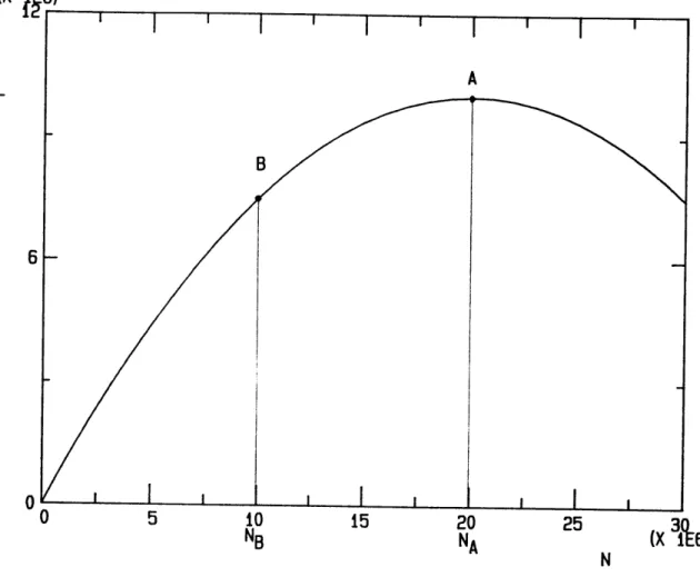
Out of the total available time after leisure, N, or the city size, gN2/2w is spent on commuting, leaving the city with the above for L. The ratio of labor to population, L/N, decreases as city size increases. The labor supply function (3.18) is a quad-ratic function the relevant portion of which is limited, of

course, to the rising part of it (see Fig. 3-1). For example, point A in Fig. 3-1 is the hypothetical extreme city size at which residents at the city edge would have to allocate all of their time to commuting and none to work. More practical limits to N are in order.

Since population density in housing is modelled to be

uniform throught the city, and since the parameter g is assumed to be invariant across city sizes, the upper bound of N is entirely determined by the situation of the person at the city

edge. That is, one must be able to trade off the lower housing rent at that location against the increased commuting time and

the consequent reduction in wage. Two reasonable behavioral assumptions are in order. We assume that on a daily basis each person sets asides 12 hours for leisure (including sleeping and other necessary daily routines) and another for work and

commut-' I I I I I I

*

I

I

j

A

B

5

10

NB

15

20

NA

25

N

Fig. 3-1: Total Labor Supply with City Size.

g/2x = 0.25x107 , NA = 2x10 ,

N

lxlO

6|

0

(X

1E6)

I

I

I

I

I

I

I

|

ing the latter of which is normalized to unity for the labor unit. We further assume that the round-trip commuting time for the resident at the edge is likely to be limited to no more than 6 hours. From (3.2) and (3.8), this means

0 < N < , (3.19)

2g

and from (3.18),

o

8g

which require that the curve of Fig. 3-1 be limited to the portion OB. Thus, at the largest practical city size, NB, for example, the city would lose 1/4 of the total available time to commuting. According to our model, if cities are endowed with equal capital per capita, K/N, large cities will have higher

capital-labor ratios, K/L, than smaller ones. This is the direct consequence of urbanization diseconomies and the other

assump-tions made for this model.

3-3. Producer Equilibrium

In the city, there are two industries, each producing a dis-tinct homogeneous good by using two homogeneous factors, labor and capital. The production function of the jth firm in the ith industry is specified to be

Y.. = A.LiK..ai, (i=1,2) (j=1,2,...,k.), (3.21)

13 1 1J 1J

0<a.<1, A.i>0,

1 1

where: Yij = output of firm j, industry i,

Lij = labor employed by firm j, industry i, Kij = capital employed by firm j, industry i, ki = number of firms in industry i.

Given that all firms within each industry are identical in size and technology, the firm production functions can be aggregated into the industry production function,

Y. = K ai, (i=1,2), (3.22)

1 11 1

where: Yi = output of industry i,

Li, Ki = labor, capital of industry i.

Into the industry production function, localization econ-omies, or what Chipman[1970] calls "parametric external economies of scale", are introduced by Ai. According to this

specifi-cation, the term Ai is viewed by the firm as a parameter, or a Hicks neutral shift factor in making its business decisions. Because the remaining elements of (3.21) constitute a homo-geneous-of-degree-one production function, the collective be-havior of the firms assures that the industries have constant-returns-to-scale production functions. This guarantees the ex-haustion of total revenues by factor payments. Thus the

com-petitition.

Although the term Ai is external to the firm, it is internal

to the industry, and is actually related to the ith industry's

output as in the following:

A.

=

Y<i,

0<.1,

(i=1,2).

(3.23)

1 1 1

This specification

conforms to our previous observation:

lo-calization economies result from the advancement of industry

output which, under spatial proximity of firms within the city,

facilitates division of labor and intra-industry specialization.

When (3.23) is substituted into (3.22), we obtain

Y

LaiIK

or

Pi,

(3.24)

1 1 1 1

~1

P. =

1

>1,

The industry production function of (3.24) is homogeneous of

degree

pi.

With pi>1 due to localization economies, it will

actually exhibit increasing returns to scale. According to

Chipman, this is called the "objective" production function,

whereas that of (3.22) is called the "subjective" production

fun-ction. The essential difference is that while the former is

based on actual production properties, the latter is based on

4 For a similar specification of external economies of scale, see

Kemp[1955,1964], Melvin[1969], and Chipman[1970], among others.

entrepreneural behavior. Not only is the term Ai external to the firms, but the relation (3.23) is assumed to be unknown to them. As we shall see later, the determination of competitive equi-librium in the presence of localization economies requires the use of both.

According to the first-order conditions for profit maximiza-tion, the reward to each factor is the value of its marginal

product to the firm, not to the industry. For such an

entrepreneural decision, therefore, we compute the marginal private, or "subjective" products of labor and capital from

(3.21), or (3.22) in the aggregate , holding Ai constant:

1Y

K. 1-a

Y

K.1-a.

L 1-a ' K 1 ) (3.25)

Substituting (3.22) into (3.25) for the elimination of Ai, we obtain aY K Jp(1-ai) Y I 8L. 1 1

ai

1p(1-ai)-1

aK. (1~ i=)L = (1-a ) K . (3.26)

11

It is to be noted that the above marginal private products of factors become less than the marginal social or "objective" products below, which can be computed directly from (3.24), by a factor of pi:

dy. Y. L= pi1i _PL L' ii Li dy. Y. 8K i K. 1

~

i1

Naturally, we assume that all marginal products are positive, finite, diminishing, and smaller than the average products.5 From (3.24), (3.26), and (3.27), this requires additional con-straints on pi as follows: p.a. <1, 1 1 (3.28) Under perfect capital rental, r, (3.26), therefore, librium conditions outputs:

competition, a uniform wage rate, w, and must prevail between the industries. From we arrive at the following producer equi-in which the factor payments exactly meet the

= _{ai--JY, K =}

(1-a i) ( lyi. (3.29)

The above producer equilibrium conditions can now be used to reveal the actual production properties via the marginal private cost curve, or the industry supply curve. Combining the objec-tive production function (3.24) and (3.29), we obtain

5 This implies that the objective production function is subject not just to increasing returns to scale, but to decreasing

returns to factor proportions as well.

(3.27)

1 . a) Y. 1

e.

w i i _{i pi.}

The supply curve has constant elasticity pi/(1-pi). Because the degree of homogeneity pi>1, the elasticity becomes negative, and the supply curve is negative-sloping. Therefore, the effect of localization economies is that at a given factor price ratio w/r, the supply price of Yi relative to the wage rate, pi/w, is

decreasing with respect to the output.

The above profit-maximizing decisions, however, also repres-ent a socially efficirepres-ent production schedule. This is because the private marginal rates of technical substitution calculated from (3.26) are identical to the social ones from (3.27):

8Y./6L. a. K. Y / 1-a. L.

1 1 1 1

Despite the presence of localization economies, production is efficient, and is operated along the city's production

possibility curve.

Although production is efficient in the sense of the identi-cal marginal rates of factor substitution for the two industries, the marginal rate of product substitution in production (or

marginal rate of transformation) is generally not equal to the price ratio. Totally differentiating (3.24) and using (3.29), we derive the following marginal rate of transformation:

dY _{p p2}

-.(3.32) = - -- dY2 2 1

This possible analytic complication, however, does not seem worth pursuing, and we limit ourselves to the kind of localization

economies which ensure equality between the marginal rate of transformation and the price ratio.6 This is possible by adding the following constraint:

p = P.

(i=1,2).

Under this assumption, of course, the ratio of marginal social costs (i.e., the slope of the production possibility curve) is equated to the ratio of marginal private costs (i.e., the price ratio which is also identical to the marginal rate of

substitu-tion in consumpsubstitu-tion). The producer equilibrium conditions of (3.29) under (3.33) now result in both production efficiency and product mix efficiency.

3-4. Market Equilibrium

Urbanization diseconomies introduced by the consumption sector, and localization economies introduced by the production sector can now be combined to show the effect of the net

6 This is mainly because our overriding concern is to investigate economic efficiency of different-sized cities and of alternative

urbanization economies on the city economy in equilibrium. In closing the model, we will first determine the factor market equilibrium under the full employment assumption, including the city's industrial composition in terms of factors, i.e., the

allocation of factors between the two industries. This will give the complete solution to the output market equilibrium. In the end, factors, products, and their prices can be solved for in terms of the city's endowments of capital and population. The prices may then be substituted into the indirect utility function which will reflect the net effect of urbanization economies and

diseconomies in terms of the exogenous variables K and N.

Our single-city model can be summarized into three sets of equations. From (3.15), the consumer equilibrium conditions,

piX. = we N 1 - N (i=1,2), (3.15)

from (3.29), the producer equilibrium conditions,

wL. rK.

piY. = . 1 (i=1,2), (3.29)

1 1

and the production possibility set, which consists of: from (3.24) and (3.33), the objective production functions; and from (3.18), the city's resource endowments,7

7 For space saving in notation, we omit subscript i in the Y sign hereafter.

Y.= LaiK 1)aiP

EL= N 1 -

gN

(i=1,2). (3.34)

K . = K,

The model is now closed by the condition that consumption of each good equals its local production, or,

X. =Y.

I 1 (i=1,2). (3.35)

Therefore, by equating (3.15) to (3.29), we get

L. = a Nf1 - + rK K =2 _{i-N +}

K.

9.Iw)Nl~

_gN

_rK)

1 rj

2x

wN)

This equilibrium allocation of factors, however, must also clear the factor markets. _{For this, we choose the labor market.} The total equilibrium labor must be the same as the city-wide labor supply. Thus, by using (3.18), (3.34) and (3.36), we obtain

L = L + L _{- Za G N 1 - +}

_rK

- N

1c..( 2 _{21 iif 2a)} (i=1,2). (3.37)

This will also determine the equilibrium factor price ratio, or the ratio of capital rental to wage rate,

r -

gN K

1 1

(U=1,2), (3.38)

parameters. _{By Walras' Law, the equilibrium factor price ratio} guarantees that capital is also fully employed. By substituting

(3.38) into (3.36), we determine Li and Ki as follows:

a.0. L. - a__ Nl -- (i=1,2), 2.27 (3.39)

K.

e

K

(i=1,2).

The above leads to this observation: in autarky equilibrium, the allocation of a factor to industry i is proportional to the

weighted average of the factor's elasticity in that industry's subjective production function, the weights being the consumer's budget shares on all goods.

The output can now be obtained by substituting (3.39) into the objective production functions (3.34):

Y.= X = 1(1 1 1iK)1-aie.Nl1 -- Nai

i a9Z(1-a ) (INJ N 2 ) *t

(i=1,2) (3.40)

The prices are now derived by substituting (3.38) and (3.40) into the demand functions (3.15):

w c9N

t

(3.41)

z(1-a.)G. p(1-a.

where c = P a a.9. Pai-1 . Kp(ai-1)

1 t hu _1-ai

n _.

that is the real price of good i in terms of labor, is determi-nate.

We now show that the equilibrium is both unique and stable by means of the supply and demand curves. Combining (3.29),

(3.34), and (3.38), we obtain the supply curves as in (3.30)

i _ (-a ) i i K -11_gN 1-ai (1-p)/p w a (1 Z)(1-a )9i N2wZ

(i=1,2),

and combining (3.15) and (3.38), we obtain the demand curves

PGl 1 1

(i=1,2). (3.43)

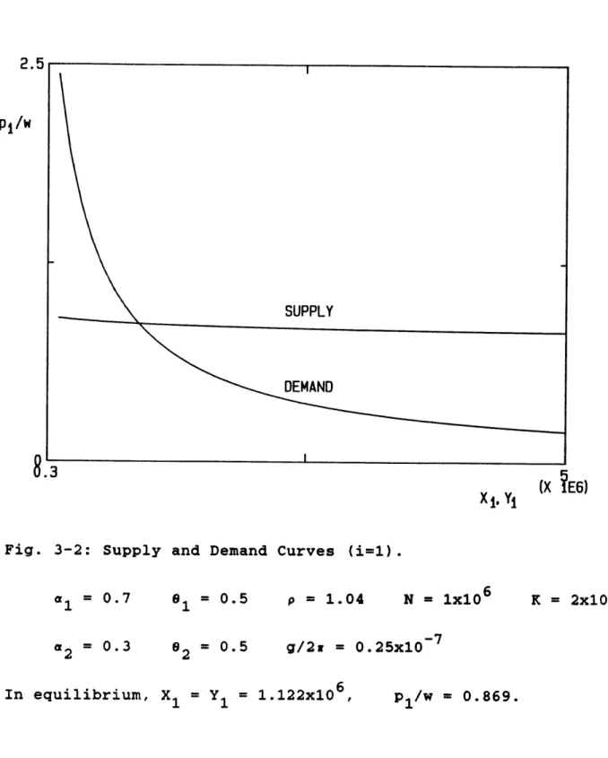
Both curves and the solution are depicted in Fig. 3-2 for in-dustry 1. The supply curve has constant elasticity p/(l-p), and the demand curve has constant elasticity -1. Since p/(l-p)<-l with p>1, the supply curve is always flatter than the demand

curve, and they meet exactly once. Therefore, the equilibrium is always unique and stable.8

8 The Marshallian stability condition is met in this typical case under external economies. Since firms will raise (lower) their output when the excess demand is positive (negative) at a given price, the equilibrium will always be restored. Under the

Walrasian stability condition in which the firms will adjust the price according to the excess demand, however, the equilibrium is unstable. Under our assumption that the firms do not re-cognize the function of (3.23), the Marshallian condition seems more appropriate.

2.5

pI

/W

Fig. 3-2: Supply and Demand Curves (i=1).

a = 0.7 a2 = 0.3 a1 = 0.5 92 = 0.5 p = 1.04 N = 1x106 K = 2x106 g/2x = 0.25x10~7 In equilibrium, X = Y = 1.122x106 ,

X1. YI

(X ?E6)

.'-3