Global Climate [in “State of the Climate in 2019"]

(1)

HAL Id: insu-02922292

https://hal-insu.archives-ouvertes.fr/insu-02922292

Submitted on 26 Aug 2020

HAL is a multi-disciplinary open access archive for the deposit and dissemination of sci-entific research documents, whether they are pub-lished or not. The documents may come from teaching and research institutions in France or abroad, or from public or private research centers.

L’archive ouverte pluridisciplinaire HAL, est destinée au dépôt et à la diffusion de documents scientifiques de niveau recherche, publiés ou non, émanant des établissements d’enseignement et de recherche français ou étrangers, des laboratoires publics ou privés.

Global Climate [in “State of the Climate in 2019”]

Robert J. H. Dunn, Diane M. Stanitski, Nadine Gobron, Kate M. Willett, M.

Ades, R. Adler, R. P. Allan, J. Anderson, Anthony Argüez, C. Arosio, et al.

To cite this version:

Robert J. H. Dunn, Diane M. Stanitski, Nadine Gobron, Kate M. Willett, M. Ades, et al.. Global Climate [in “State of the Climate in 2019”]. Bulletin of the American Meteorological Society, American Meteorological Society, 2020, 101 (8), pp.S9-S127. �10.1175/BAMS-D-20-0104.1�. �insu-02922292�

(2)

S9

2 . G L O BA L C L I M AT E AU G U S T 2 0 2 0 | S t a t e o f t h e C l i m a t e i n 2 0 1 9

GLOBAL CLIMATE

R. J. H. Dunn, D. M. Stanitski, N. Gobron, and K. M. Willett, Eds.

STATE OF THE CLIMATE IN 2019

Special Online Supplement to the Bulletin of the American Meteorological Society, Vol.101, No. 8, August, 2020 https://doi.org/10.1175/BAMS-D-20-0104.1

For information regarding reuse of this content and general copyright information, consult the AMS Copyright Policy.

(3)

S10

STATE OF THE CLIMATE IN 2019

Global Climate

Editors

Jessica Blunden

Derek S. Arndt

Chapter Editors

Peter Bissolli

Howard J. Diamond

Matthew L. Druckenmiller

Robert J. H. Dunn

Catherine Ganter

Nadine Gobron

Rick Lumpkin

Jacqueline A. Richter-Menge

Tim Li

Ademe Mekonnen

Ahira Sánchez-Lugo

Ted A. Scambos

Carl J. Schreck III

Sharon Stammerjohn

Diane M. Stanitski

Kate M. Willett

Technical Editor

Andrea Andersen

BAMS Special Editor for Climate

Richard Rosen

American Meteorological Society

(4)

S11

Cover credit:

The cover shows a cropped image of the warming stripes (seen in full below), as developed by Ed Hawkins (Reading University, UK). Each vertical line shows the global average temperature of a whole year, starting at 1850 on the far left and ending with 2019 on the far right. The un-derlying data are from the HadCRUT4.6 dataset of the UK Met Office Hadley Centre. To create stripes of other regions and countries visit https://showyourstripes.info/. Image created on 23 June 2020 by https://showyourstripes.info/ under a CC BY 4.0 licence.

Global Climate is one chapter from the State of the Climate in 2019 annual report and is avail-able from https://doi.org/10.1175/BAMS-D-20-0104.1 Compiled by NOAA’s National Centers for Environmental Information, State of the Climate in 2019 is based on contributions from scien-tists from around the world. It provides a detailed update on global climate indicators, notable weather events, and other data collected by environmental monitoring stations and instru-ments located on land, water, ice, and in space.

The full report is available from https://doi.org/10.1175/2020BAMSStateoftheClimate.1. How to cite this document:

Citing the complete report:

Blunden, J. and D. S. Arndt, Eds., 2020: State of the Climate in 2019. Bull. Amer. Meteor., 101 (8), Si–S429 doi:10.1175/2020BAMSStateoftheClimate.1

Citing this chapter:

Dunn, R. J. H., D. M. Stanitski, N. Gobron, and K. M. Willett, Eds., 2020: Global Climate [in “State of the Climate in 2019"]. Bull. Amer. Meteor., 101 (8), S9–S127, https://doi.org/10.1175/BAMS-D-20-0104.1

Citing a section (example):

Davis, M., K. H. Rosenlof, D. F. Hurst, H. Vömel, and H.B. Selkirk, 2020: Stratospheric water vapor [in “State of the Climate in 2019"]. Bull. Amer. Meteor., 101 (8), S81–S83, https://doi.org/10.1175/ BAMS-D-20-0104.1.

(5)

S12

Editor and Author Affiliations (alphabetical by name)

Ades, M., European Centre for Medium-Range Weather Forecasts, Reading, United Kingdom

Adler, R., University of Maryland, College Park, Maryland Allan, Rob, Met Office Hadley Centre, Exeter, United Kingdom Allan, R. P., University of Reading, Reading, United Kingdom

Anderson, J., Department of Atmospheric and Planetary Science, Hampton University, Hampton, Virginia

Argüez, Anthony, NOAA/NESDIS National Centers for Environmental Information, Asheville, North Carolina

Arosio, C., University of Bremen, Bremen, Germany

Augustine, J. A., NOAA/OAR Earth System Research Laboratories, Boulder, Colorado

Azorin-Molina, C., Centro de Investigaciones sobre Desertificación – Spanish National Research Council, Moncada (Valencia), Spain; and Regional Climate Group, Department of Earth Sciences, University of Gothenburg, Gothenburg, Sweden

Barichivich, J., Instituto de Geografía, Pontificia Universidad Católica de Valparaíso, Valparaíso, Chile

Barnes, J., NOAA/OAR ESRL Global Monitoring Laboratory, Boulder, Colorado Beck, H. E., Department of Civil and Environmental Engineering, Princeton

University, Princeton, New Jersey

Becker, Andreas, Global Precipitation Climatology Centre, Deutscher Wetterdienst, Offenbach, Germany

Bellouin, Nicolas, University of Reading, Reading, United Kingdom Benedetti, Angela, European Centre for Medium-Range Weather Forecasts,

Reading, United Kingdom

Berry, David I., National Oceanography Centre, Southampton, United Kingdom Blenkinsop, Stephen, School of Engineering, Newcastle University,

Newcastle-upon-Tyne, United Kingdom

Bock, Olivier, Université de Paris, Institut de physique du globe de Paris, CNRS, IGN, Paris, France, and ENSG-Géomatique, IGN, Marne-la-Vallée, France Bosilovich, Michael G., Global Modeling and Assimilation Office, NASA

Goddard Space Flight Center, Greenbelt, Maryland Boucher, Olivier, Sorbonne Université, Paris, France Buehler, S. A., Universität Hamburg, Hamburg, Germany Carrea, Laura, Department of Meteorology, University of Reading,

Christiansen, Hanne H., Geology Department, University Centre in Svalbard, Longyearbyen, Norway

Chouza, F., Jet Propulsion Laboratory, California Institute of Technology, Wrightwood, California

Christy, John R., The University of Alabama in Huntsville, Huntsville, Alabama Chung, E.-S., IBS Center for Climate Physics, Busan, South Korea

Coldewey-Egbers, Melanie, German Aerospace Center (DLR) Oberpfaffenhofen, Wessling, Germany

Compo, Gil P., Cooperative Institute for Research in Environmental Sciences, University of Colorado Boulder, and Physical Sciences Division, NOAA/Earth System Research Laboratory, Boulder, Colorado

Cooper, Owen R., Cooperative Institute for Research in Environmental Sciences, University of Colorado Boulder, and NOAA/OAR Earth System Research Laboratories, Boulder, Colorado

Covey, Curt, Lawrence Livermore National Laboratory, Livermore, California Crotwell, A., Cooperative Institute for Research in Environmental Sciences,

University of Colorado, and NOAA/OAR Global Monitoring Division, Boulder, Colorado

Davis, Sean M., Cooperative Institute for Research in Environmental Sciences, University of Colorado Boulder, and NOAA/OAR Earth System Research Laboratory, Boulder, Colorado

de Eyto, Elvira, Marine Institute, Furnace, Newport, Ireland

de Jeu, Richard A. M., VanderSat B.V., Haarlem, the Netherlands DeGasperi, Curtis L., King County Water and Land Resources Division,

Seattle, Washington

Degenstein, Doug, University of Saskatchewan, Saskatoon, Saskatchewan, Canada

Di Girolamo, Larry, University of Illinois at Urbana-Champaign, Champaign, Illinois

Dokulil, Martin T., Research Department for Limnology, University of Innsbruck, Austria

Donat, Markus G., Barcelona Supercomputing Centre, Barcelona, Spain Dorigo, Wouter A., Department of Geodesy and Geoinformation, TU Wien -

Vienna University of Technology, Vienna, Austria

Dunn, Robert J. H., Met Office Hadley Centre, Exeter, United Kingdom Durre, Imke, NOAA/NESDIS National Centers for Environmental Information,

Asheville, North Carolina

Dutton, Geoff S., Cooperative Institute for Research in Environmental Sciences, University of Colorado Boulder, and NOAA/OAR Earth System Research Laboratories, Boulder, Colorado

Duveiller, G., European Commission, Joint Research Centre, Ispra, Italy Elkins James W., NOAA/OAR Earth System Research Laboratories,

Boulder, Colorado,

Fioletov, Vitali E., Environment and Climate Change Canada, Toronto, Canada Flemming, Johannes, European Centre for Medum-Range Weather Forecasts,

Foster, Michael J., Cooperative Institute for Meteorological Satellite Studies, Space Science and Engineering Center, University of Wisconsin-Madison, Madison, Wisconsin

Frey, Richard A., Cooperative Institute for Meteorological Satellite Studies, Space Science and Engineering Center, University of Wisconsin-Madison, Madison, Wisconsin

Frith, Stacey M., Science Systems and Applications, Inc, Lanham, Maryland, NASA Goddard Space Flight Center, Greenbelt, Maryland

Froidevaux, Lucien, Jet Propulsion Laboratory, California Institute of Technology, Pasadena, California

Garforth, J., Woodland Trust, Grantham, United Kingdom

Gobron, Nadine, European Commission, Joint Research Centre, Ispra, Italy Gupta, S. K., Science Systems and Applications, Inc., Hampton, Virginia Haimberger, Leopold, Department of Meteorology and Geophysics, University

of Vienna, Vienna, Austria

Hall, Brad D., NOAA/OAR Earth System Research Laboratories, Boulder, Colorado

Harris, Ian, National Centre for Atmospheric Science (NCAS), University of East Anglia, Norwich, United Kingdom and Climatic Research Unit, School of Environmental Sciences, University of East Anglia, Norwich, United Kingdom Heidinger, Andrew K., NOAA/NESDIS/STAR University of Wisconsin - Madison,

Madison, Wisconsin

Hemming, D. L., Met Office Hadley Centre, Exeter, United Kingdom; Birmingham Institute of Forest Research, Birmingham University, Birmingham, United Kingdom

Ho, Shu-peng (Ben), NOAA/NESDIS Center for Satellite Applications and Research, College Park, Maryland

Hubert, Daan, Royal Belgian Institute for Space Aeronomy (BIRA), Brussels, Belgium

Hurst, Dale F., Cooperative Institute for Research in Environmental Sciences, University of Colorado Boulder, and NOAA/OAR Earth System Research Laboratories, Boulder, Colorado

Hüser, I., Deutscher Wetterdienst, Offenbach, Germany

Inness, Antje, European Centre for Medium Range Weather Forecasts, Reading, United Kingdom

(6)

S13

Editor and Author Affiliations (alphabetical by name)

Isaksen, K., Norwegian Meteorological Institute, Blindern, Oslo, Norway John, Viju, EUMETSAT, Darmstadt, Germany

Jones, Philip D., Climatic Research Unit, School of Environmental Sciences, University of East Anglia, Norwich, United Kingdom

Kaiser, J. W., Deutscher Wetterdienst, Offenbach, Germany Kelly, S., Dundalk Institute of Technology, Dundalk, Ireland Khaykin, S., LATMOS/IPSL, UVSQ, Sorbonne Université, CNRS,

Guyancourt, France

Kidd, R., Earth Observation Data Centre GmbH, Vienna, Austria Kim, Hyungiun, Institite of Industrial Science, The University of Tokyo,

Tokyo, Japan

Kipling, Z., European Centre for Medium-Range Weather Forecasts, Reading, United Kingdom

Kraemer, B. M., IGB Leibniz Institute for Freshwater Ecology and Inland Fisheries, Berlin, Germany

Kratz, D. P., NASA Langley Research Center, Hampton, Virginia La Fuente, R. S., Dundalk Institute of Technology, Dundalk, Ireland Lan, Xin, Cooperative Institute for Research in Environmental Sciences,

University of Colorado Boulder, and NOAA/OAR Earth System Research Laboratories, Boulder, Colorado

Lantz, Kathleen O., NOAA/OAR Earth System Research Laboratory, and Cooperative Institute for Research in the Environmental Sciences, University of Colorado, Boulder, Colorado

Leblanc, T., Jet Propulsion Laboratory, California Institute of Technology, Wrightwood, California

Li, Bailing, Hydrological Sciences Laboratory, NASA Goddard Space Flight Center, Greenbelt, Maryland, USA; Earth System Science Interdisciplinary Center, University of Maryland, College Park, Maryland

Loeb, Norman G., NASA Langley Research Center, Hampton, Virginia Long, Craig S., NOAA/NWS National Centers for Environmental Prediction,

College Park, Maryland

Loyola, Diego, German Aerospace Center (DLR) Oberpfaffenhofen, Wessling, Germany

Marszelewski, Wlodzimierz, Department of Hydrology and Water Management, Nicolaus Copernicus University, Toruń, Poland Martens, B., Hydro-Climate Extremes Lab (H-CEL), Ghent University,

Ghent, Belgium

May, Linda, Centre for Ecology & Hydrology, Edinburgh, United Kingdom Mayer, Michael, Department of Meteorology and Geophysics, University of

Vienna, Austria; European Centre for Medium-Range Weather Forecasts, Reading, United Kingdom

McCabe, M. F., Division of Biological and Environmental Sciences and Engineering, King Abdullah University of Science and Technology, Thuwal, Saudi Arabia

McVicar, Tim R., CSIRO Land and Water, Canberra, Australian Capital Territory; and Australian Research Council Centre of Excellence for Climate Extremes, Sydney, New South Wales, Australia

Mears, Carl A., Remote Sensing Systems, Santa Rosa, California Menzel, W. Paul, Space Science and Engineering Center, University of

Wisconsin-Madison, Madison, Wisconsin

Merchant, Christopher J., Department of Meteorology, and National Centre for Earth Observation, University of Reading, Reading, United Kingdom Miller, Ben R., Cooperative Institute for Research in Environmental Sciences,

University of Colorado Boulder, and NOAA/OAR Earth System Research Laboratories, Boulder, Colorado

Miralles, Diego G., Hydro-Climate Extremes Lab (H-CEL), Ghent University, Ghent, Belgium

Montzka, Stephen A., NOAA/OAR Earth System Research Laboratories, Boulder, Colorado

Morice, Colin, Met Office Hadley Centre, Exeter, United Kingdom

Mühle, Jens, Scripps Institution of Oceanography, University of California, San Diego, La Jolla, California

Myneni, R., Department of Earth and Environment, Boston University, Boston, Massachusetts

Nicolas, Julien P., European Centre for Medium-Range Weather Forecasts, Reading, United Kingdom

Noetzli, Jeannette, WSL Institute for Snow and Avalanche Research SLF, Davos-Dorf, Switzerland

Osborn, Tim J., Climatic Research Unit, School of Environmental Sciences, University of East Anglia, Norwich, United Kingdom

Park, T., NASA Ames Research Center, and Bay Area Environmental Research Institute, Moffett Field, California

Pasik, A., Department of Geodesy and Geoinformation, TU Wien - Vienna University of Technology, Vienna, Austria

Paterson, Andrew M., Dorset Environmental Science Centre, Ontario Ministry of the Environment and Climate Change, Dorset, Ontario, Canada Pelto, Mauri S., Nichols College, Dudley, Massachusetts

Perkins-Kirkpatrick, S., University of New South Wales, Sydney, Australia Pétron, G., Cooperative Institute for Research in Environmental Sciences,

University of Colorado, and NOAA/OAR Global Monitoring Laboratory, Boulder, Colorado

Phillips, C., Department of Atmospheric and Oceanic Sciences, University of Wisconsin-Madison, Madison, Wisconsin

Pinty, Bernard, European Commission, Joint Research Centre, Ispra, Italy Po-Chedley, S., Lawrence Livermore National Laboratory, Livermore, California Polvani, L., Columbia University, New York, New York

Preimesberger, W., Department of Geodesy and Geoinformation, TU Wien - Vienna University of Technology, Vienna, Austria

Pulkkanen, M., Finnish Environment Institute SYKE, Freshwater Centre, Helsinki, Finland.

Randel, W. J., National Center for Atmospheric Research, Boulder, Colorado Rémy, Samuel, Institut Pierre-Simon Laplace, CNRS / UPMC, Paris, France Ricciardulli, L., Remote Sensing Systems, Santa Rosa, California

Richardson, A. D., School of Informatics, Computing, and Cyber Systems and Center for Ecosystem Science and Society, Northern Arizona University, Flagstaff, Arizona

Rieger, L., University of Saskatchewan, Saskatoon, Canada Robinson, David A., Department of Geography, Rutgers University,

Piscataway, New Jersey

Rodell, Matthew, Hydrological Sciences Laboratory, NASA Goddard Space Flight Center, Greenbelt, Maryland

Rosenlof, Karen H., NOAA/OAR Earth System Research Laboratories, Boulder, Colorado

Roth, Chris, University of Saskatchewan, Saskatoon, Saskatchewan, Canada Rozanov, A., University of Bremen, Bremen, Germany

Rusak, James A., Dorset Environmental Science Centre, Ontario Ministry of the Environment and Climate Change, Dorset, Ontario, Canada

Rusanovskaya, O., Institute of Biology, Irkutsk State University, Russia Rutishäuser, T., Institute of Geography and Oeschger Center, University of

Berne, Berne, Switzerland

Sánchez-Lugo, Ahira, NOAA/NESDIS National Centers for Environmental Information, Asheville, North Carolina

Sawaengphokhai, P., Science Systems and Applications, Inc., Hampton, Virginia

Scanlon, T., Department of Geodesy and Geoinformation, TU Wien - Vienna University of Technology, Vienna, Austria

Schenzinger, Verena, Department of Meteorology and Geophysics, University of Vienna, Austria

(7)

S14

Editor and Author Affiliations (alphabetical by name)

Schladow, S. Geoffey, Tahoe Environmental Research Center, University of California at Davis, Davis, California

Schlegel, R. W., Physical Oceanography Department, Woods Hole Oceanographic Institution, Woods Hole, Massachusetts

Schmid, Martin, Eawag, Swiss Federal Institute of Aquatic Science and Technology, Kastanienbaum, Switzerland

Selkirk, H. B., Universities Space Research Association, NASA Goddard Space Flight Center, Greenbelt, Maryland

Sharma, S., York University, Toronto, Ontario, Canada

Shi, Lei, NOAA/NESDIS, National Centers for Environmental Information, Asheville, North Carolina

Shimaraeva, S. V., Institute of Biology, Irkutsk State University, Russia Silow, E. A., Institute of Biology, Irkutsk State University, Russia

Simmons, Adrian J., European Centre for Medium-Range Weather Forecasts, Reading, United Kingdom

Smith, C. A., Cooperative Institute for Research in Environmental Sciences, University of Colorado Boulder, and Physical Sciences Laboratory, NOAA/ Earth System Research Laboratories, Boulder, Colorado

Smith, Sharon L., Geological Survey of Canada, Natural Resources Canada, Ottawa, Ontario, Canada

Soden, B. J., Rosenstiel School of Marine and Atmospheric Science, University of Miami, Key Biscayne, Florida

Sofieva, Viktoria, Finnish Meteorological Institute (FMI), Helsinki, Finland Sparks, T. H., Poznań University of Life Sciences, Poznań, Poland

Stackhouse, Jr., Paul W., NASA Langley Research Center, Hampton, Virginia Stanitski, Diane M., NOAA/OAR Earth System Research Laboratories,

Boulder, Colorado

Steinbrecht, Wolfgang, German Weather Service (DWD), Hohenpeissenberg, Germany

Streletskiy, Dimitri A., Department of Geography George Washington University, Washington D.C.

Taha, G., GESTAR, Columbia, Maryland

Telg, Hagen, NOAA/OAR Earth System Research Laboratories and Cooperative Institute for Research in the Environmental Sciences, University of Colorado, Boulder, Colorado

Thackeray, S. J., Centre for Ecology and Hydrology, Lancaster, United Kingdom Timofeyev, M. A., Institute of Biology, Irkutsk State University, Russia Tourpali, Kleareti, Aristotle University, Thessaloniki, Greece

Tye, Mari R., Capacity Center for Climate and Weather Extremes (C3WE), National Center for Atmospheric Research, Boulder, Colorado van der A, Ronald J., Royal Netherlands Meteorological Institute (KNMI),

De Bilt, Netherlands

van der Schalie, Robin, VanderSat B.V., Haarlem, Netherlands

van der Schrier, Gerard, Royal Netherlands Meteorological Institute (KNMI), De Bilt, Netherlands

van der Werf, Guido R., Vrije Universiteit Amsterdam, Amsterdam, Netherlands

Verburg, Piet, National Institute of Water and Atmospheric Research, Hamilton, New Zealand

Vernier, Jean-Paul, NASA Langley Research Center, Hampton, Virginia Vömel, Holger, Earth Observing Laboratory, National Center for Atmospheric

Research, Boulder, Colorado

Vose, Russell S., NOAA/NESDIS National Centers for Environmental Information, Asheville, North Carolina

Wang, Ray, Georgia Institute of Technology, Atlanta, Georgia

Watanabe, Shohei G., Tahoe Environmental Research Center, University of California at Davis, Davis, California

Weber, Mark, University of Bremen, Bremen, Germany

Weyhenmeyer, Gesa A., Department of Ecology and Genetics/Limnology, Uppsala University, Uppsala, Sweden

Wiese, David, Jet Propulsion Laboratory, California Institute of Technology, Pasadena, California

Wilber, Anne C., Science Systems and Applications, Inc., Hampton, Virginia Wild, Jeanette D., NOAA Climate Prediction Center, College Park, Maryland;

ESSIC/University of Maryland, College Park, Maryland Willett, Kate M., Met Office Hadley Centre, Exeter, United Kingdom Wong, Takmeng, NASA Langley Research Center, Hampton, Virginia Woolway, R. Iestyn, Dundalk Institute of Technology, Dundalk, Ireland Yin, Xungang, ERT Inc., NOAA/NESDIS National Centers for Environmental

Information, Asheville, North Carolina

Zhao, Lin, School of Geographical Sciences, Nanjing University of Information Science & Technology, Nanjing, China

Zhao, Guanguo, University of Illinois at Urbana-Champaign, Champaign, Illinois

Zhou, Xinjia, Center for Satellite Applications and Research, NOAA, College Park, Maryland

Ziemke, Jerry R., Goddard Earth Sciences Technology and Research, Morgan State University, Baltimore, Maryland, and NASA Goddard Space Flight Center, Greenbelt, Maryland

Ziese, Markus, Global Precipitation Climatology Center, Deutscher Wetterdienst, Offenbach am Main, Germany

Editorial and Production Team

Andersen, Andrea, Technical Editor, Innovative Consulting Management Services, LLC, NOAA/NESDIS National Centers for Environmental Information, Asheville, North Carolina

Griffin, Jessicca, Graphics Support, Cooperative Institute for Satellite Earth System Studies, North Carolina State University, Asheville, North Carolina

Hammer, Gregory, Content Team Lead, Communications and Outreach, NOAA/NESDIS National Centers for Environmental Information, Asheville, North Carolina

Love-Brotak, S. Elizabeth, Lead Graphics Production, NOAA/NESDIS National Centers for Environmental Information, Asheville, North Carolina

Misch, Deborah J., Graphics Support, Innovative Consulting Management Services, LLC, NOAA/NESDIS National Centers for Environmental Information, Asheville, North Carolina

Riddle, Deborah B., Graphics Support, NOAA/NESDIS National Centers for Environmental Information, Asheville, North Carolina

Veasey, Sara W., Visual Communications Team Lead, Communications and Outreach, NOAA/NESDIS National Centers for Environmental Information, Asheville, North Carolina

(8)

S15

List of authors and affiliations ...S13 a. Overview. ...S17 b. Temperature. ... S24 1. Global surface temperature ... S24 2. Lake surface temperature... S26 3. Land and marine temperature extremes ... S28 4. Tropospheric temperature ... S30 5. Stratospheric temperature ... S32 c. Cryosphere ... S34 1. Permafrost thermal state... S34 2. Northern Hemisphere snow cover extent ... S36 3. Glaciers ... S37 Sidebar 2.1: Lake ice ... S39 d. Hydrological cycle ... S42 1. Surface humidity ... S42 2. Total column water vapor ... S44 3. Upper tropospheric humidity ... S45 4. Precipitation ... S46 5. Land surface precipitation extremes ... S47 6. Lake water levels ... S49 7. Global cloudiness ...S51 8. River discharge and runoff ... S53 9. Groundwater and terrestrial water storage ... S55 10. Soil moisture ... S56 11. Land evaporation ... S57 12. Monitoring global drought using the self-calibrating

Palmer Drought Severity Index ... S59 e. Atmospheric circulation. ... S60 1. Mean sea level pressure and related modes of variability ... S60 2. Land and ocean surface winds ... S63 3. Upper air winds ... S65 f. Earth radiation budget ... S66 1. Earth radiation budget at top of atmosphere ... S66 2. Mauna Loa clear-sky “apparent” solar transmission ... S69

2. Table of Contents

(9)

S16

g. Atmospheric composition ... S70 1. Long-lived greenhouse gases ... S70 2. Ozone-depleting substances ... S75 3. Aerosols ... S76 4. Stratospheric ozone ... S78 5. Stratospheric water vapor ... S81 6. Tropospheric ozone ... S83 7. Carbon monoxide ... S86 Sidebar 2.2: 2019: A 25-year high in global stratospheric aerosol loading ... S88 h. Land surface properties ... S90 1. Land surface albedo dynamics ... S90 2. Terrestrial vegetation dynamics ... S92 3. Biomass burning ... S93 4. Phenology of primary producers ... S95 Acknowledgments ... S99 Appendix 1: Acronym List... ...S102 Appendix 2: Supplemental Material... ...S105 References... ... S117

*Please refer to Chapter 8 (Relevant datasets and sources) for a list of all climate variables and datasets used in this chapter for analyses, along with their websites for more information and access to the data.

2. Table of Contents

(10)

S17

a. Overview—R. J. H. Dunn, D. M. Stanitski, N. Gobron, and K. M. Willett

The assessments and analyses presented in this chapter focus predominantly on the measured differences of climate and weather observables from previous conditions, years, and decades to place 2019 in context. Many of these differences have direct impacts on people, for example, their health and environment, as well as the wider biosphere, but are beyond the scope of these analyses.

For the last few State of the Climate reports, an update on the number of warmer-than-average years has held no surprises, and this year is again no different. The year 2019 was among the three warmest years since records began in the mid-to-late 1800s. Only 2016, and for some datasets 2015, were warmer than 2019; all years after 2013 have been warmer than all others back to the mid-1800s. Each decade since 1980 has been successively warmer than the preceding decade, with the most recent (2010–19) being around 0.2°C warmer than the previous (2000–09).

This warming of the land and ocean surface is reflected across the globe. For example, lake and permafrost temperatures have increased; glaciers have continued to lose mass, becoming thinner for the 32nd consecutive year, with the majority also becoming shorter during 2019. The period during which Northern Hemisphere (NH) lakes were covered in ice was seven days shorter than the 1981–2010 long-term average, based on in situ phenological records. There were fewer cool extremes and more warm extremes on land; regions including Europe, Japan, Pakistan, and India all experienced heat waves. More strong than moderate marine heat waves were recorded for the sixth consecutive year. And in Australia (discussed in more detail in section 7h4), moisture deficits and prolonged high temperatures led to severe impacts during late austral spring and summer, including devastating wildfires. Smoke from these wildfires was detected across large parts of the Southern Hemisphere (SH).

The year 2019 was also one of the three warmest above Earth’s surface and within the tropo-sphere, while middle and upper stratospheric temperatures were at their lowest recorded values since 1979, as is expected because of the increasing concentration of greenhouse gases in the atmosphere.

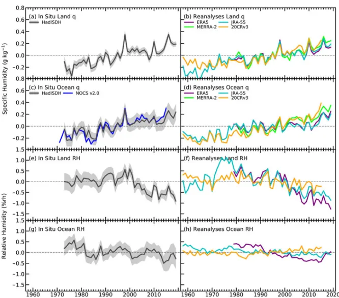
The continuing warm conditions also influenced water around the globe, with atmospheric water vapor (specific humidity) being high over the ocean surface (one of the moistest years on record) and also aloft, and well above average near the land surface. However, in terms of satura-tion (relative humidity), the atmosphere was very dry near the land surface, setting a new record low for the global average, and about average over the ocean surface and aloft. There were strong hemispheric differences in soil moisture anomalies with, on average, negative anomalies in the south and positive anomalies in the north. Globally, the second half of 2019 saw an increase in the land area experiencing drought to higher, but not record, levels by the end of the year, but annual precipitation amounts were around average, with regional peaks in intense rainfall from, for example, Cyclones Idai and Kenneth in southeastern Africa.

Many climate events in Africa, Asia, and Australia were influenced by the strong positive Indian Ocean dipole (IOD), while the weak-to-neutral prolonged El Niño–Southern Oscillation (ENSO) conditions during 2019 appeared to have only limited impacts.

2. GLOBAL CLIMATE

R. J. H. Dunn, D. M. Stanitski, N. Gobron, and K. M. Willett, Eds.

(11)

S18

As a primary driver for our changing climate, the abundance of many long-lived greenhouse gases continues to increase. Globally averaged CO2 at Earth’s surface reached 409.8 ± 0.1 ppm,

a 2.5 ± 0.1 ppm increase from 2018; and CH₄ reached 1866.6 ± 0.9 ppb in 2019, a 9.2 ± 0.9 ppb increase from 2018, which is among the three largest annual increases (with 2014 and 2015) since 2007, when a rapid rise in methane concentration began. The mean global atmospheric N2O abundance

in 2019 was 331.9 ± 0.1 ppb, an increase of 1.0 ± 0.2 ppb from 2018. However, the atmospheric abundances of most ozone-depleting substances (ODS) are declining or leveling off, decreasing the stratospheric halogen loading and radiative forcing associated with ODS.

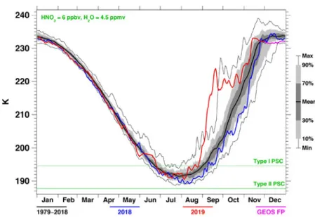
Stratospheric water vapor variability is strongly affected by the absolute humidity of air enter-ing the stratosphere in the tropics, which is in turn largely determined by the temperature of the tropical cold point tropopause. Following 2018, a year in which lower stratospheric water vapor in the tropics dropped to a very low value (~20% below the 2004–19 average in December), water vapor abundance in the tropical lower stratosphere increased during 2019 to about 10% above average in the latter half of the year.

Both hemispheric average and global average tropospheric ozone in 2019 indicate a continuing increase from previous years based on satellite measurements (starting year 2004) and surface measurements (starting in the mid-1970s). The largest trends in tropospheric ozone over the last 15 years occurred above India and East/Southeast Asia at a rate of ~ +3.3 DU decade−1_{(~ +1% yr}−1_);

these increases are consistent with expected increases of ozone precursor emissions across this region.

The year saw exceptional fire events over Australia, Indonesia, and parts of Siberia, but was also marked by lower amounts of dust over most of the Sahara. In the latter part of 2019, the Raikoke (Russia) and Ulawun (Papua New Guinea) volcanic eruptions and the large Australian wildfires loaded the stratosphere with aerosol levels unprecedented since the post-Mt. Pinatubo era 25 years ago. Despite this, 2019 was near-record warm at the surface.

The responses of the terrestrial biosphere to climatic conditions were also visible. Phenological land indicators show an average excess of eight days for the duration of the growing season in the NH in 2019 relative to the 2000–10 baseline. A deficit of plant productivity in the SH resulted in a lighter surface and hence higher albedo, whereas northern latitudes presented a darker surface and lower albedo, largely due to below-average snow cover. However, the rate of photosynthesis increased in eastern China with vegetation growth due to major human changes in land use.

New additions to this chapter in 2019 include lake water levels (last included in 2011) and side-bars on lake ice cover and stratospheric aerosols. Marine temperature extremes are also included this year alongside the land–surface indices, and we see the return of an update on the Mauna Loa solar transmission record.

Time series and anomaly maps for many of the variables described in this chapter are shown in Plates 1.1 and 2.1, respectively. A number of sections refer to supplemental figures that can be found in Appendix 2.

(12)

S19

Plate 2.1. (a) NOAA NCEI Global land and ocean surface annual temperature anomalies (°C); (b) Satellite-derived lake surface water temperature anomalies (°C) in 2019. The anomalies are calculated for the meteorological warm season (JJA in NH; DJF in SH, and over Dec–Aug 2018/19 within 23.5° of the equator). The longitude of some of the lakes has been shifted slightly to enable them to be displayed clearly. The latitude has been maintained; (c) GHCNDEX warm day threshold exceedance (TX90p); (d) GHCNDEX cool night threshold exceedance (TN10p); (e) ERA5 annual temperature anomalies of LTT (°C). Stippling indicates grid points in which the 2019 value was the highest of the 41-year record; (f) ERA5 annual temperature anomalies of LST (°C); (g) HadISDH surface specific humidity anomalies (g kg–1_);

(13)

S20

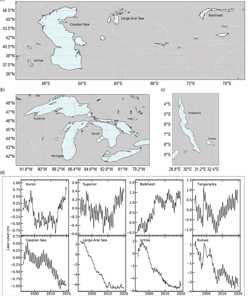
Plate 2.1. (cont.) (h) HadISDH surface relative humidity anomalies (% RH); (i) ERA5 reanalysis of TCWV anomalies (mm). Data from GNSS stations are plotted as filled circles; (j) “All sky” microwave-based UTH dataset annual average UTH anomalies (% RH); (k) GPCP v2.3 annual mean precipita-tion anomalies for 2019 (mm yr−1_{); (l) Anomalies for the 2019} GPCC-First Guess Daily R10mm index (days); (m) Lake water level anomalies (meters) based on satellite altimeters for 198 large lakes; (n) Global cloudiness anomalies (%) generated from the 30-year PATMOS-x /AVHRR cloud climatology;

(14)

S21

Plate 2.1. (cont.) (o) Global distribution of river discharge anomalies (m3_s−1_{) from JRA-55; (p) Global} distribution of runoff anomalies (mm yr−1_{) from JRA-55; (q) Changes in annual-mean terrestrial water} storage (the sum of groundwater, soil water, surface water, snow, and ice, as an equivalent height of water in cm) between 2018 and 2019, based on output from a GRACE and GRACE-FO data-assimilating land surface model. No data are shown over Greenland, Antarctica, the gulf coast of Alaska, parts of Patagonia, and most polar islands; (r) ESA CCI Soil Moisture average surface soil moisture anomalies (m3_m−3_{). Data were masked as missing where retrievals are either not possible or of very low} qual-ity (dense forests, frozen soil, snow, ice, etc.); (s) GLEAM land evaporation anomalies (mm yr−1_{); (t)} Mean scPDSI for 2019. Droughts are indicated by negative values (brown), wet episodes by positive values (green). No calculation is made where a drought index is meaningless (gray areas: ice sheets or deserts with approximately zero mean precipitation);

(15)

S22

Plate 2.1. (cont.) (u) HadSLP2r surface pressure anomalies (hPa); (v) Surface wind speed anomalies (m s−1_{) from the observational HadISD3 dataset (land, circles), the MERRA-2 reanalysis output (land,} shaded areas), and RSS satellite observations (ocean, shaded areas); (w) ERA5 Aug–Dec average 850-hPa eastward wind speed anomalies (m s−1_{); (x) Total aerosol optical depth (AOD) anomalies at 550 nm; (y)} Number of days with extremely high AOD (extreme being defined as above the local 99.9th percentile of the 2003–18 average; (z) Total column ozone anomalies (DU) in 2019 from Global Ozone Monitor-ing Experiment-2 (GOME-2A) measurements with respect to the 1998–2008 mean determined from the merged multi-sensor data combining GOME, SCIAMACHY, and GOME-2 (GSG, Weber et al. 2018);

(16)

S23

Plate 2.1. (cont.) (aa) Tropospheric ozone anomalies (DU) for 2019, relative to 2005–18 average, as de-tected by the OMI/MLS satellite instruments; (ab) CAMS reanalysis total column CO anomalies (%); (ac) Land surface visible albedo anomalies (%); (ad) Land surface near-infrared albedo anomalies (%); (ae) FAPAR anomalies; (af) GFAS1.4 carbonaceous emission anomalies (g C m−2_yr−1_{) from biomass burning.}

(17)

S24

b. Temperature

1) Global surface temperature— A. Sánchez-Lugo, C. Morice, J. P. Nicolas, and A. Argüez

The 2019 global land and ocean surface temperature was 0.44°–0.56°C above the 1981–2010 average (Table 2.1) and was among the three high-est yearly temperatures since global records began in the mid-to-late 1800s (Fig. 2.1), according to three independent in situ analyses (NASA-GISS, Lenssen et al. 2019; HadCRUT4, Morice et al. 2012; NOAAGlobalTemp, H.-M. Zhang et al. 2019). The NOAAGlobalTemp and NASA-GISS datasets ranked 2019 as the second-warmest year on record, just 0.04°C behind 2016. The HadCRUT4 da-taset ranked 2019 as the third-warmest year, behind 2016 (+0.50°C) and 2015 (+0.47°C). A weak El Niño was present across the tropical Pacific Ocean at the start of the year (see section 4b). The presence of an El Niño (La Niña) typi-cally has a warming (cooling) influence on global temperatures (e.g., Foster and Rahmstorf 2011). The El Niño transi-tioned to El Niño–Southern Oscillation (ENSO) neutral by mid-2019.

The three in situ global surface tem-perature analyses assessed here are derived from air temperatures observed at weather stations over land and sea surface temperatures (SSTs) observed from ships and buoys. Differences be-tween analyses are mainly due to how each methodology treats areas with little to no data and how each analysis accounts for changes in measurement methods (for more details see Kennedy et al. [2010]; Hansen et al. [2010]; and Sánchez-Lugo et al. [2017]). Although each analysis differs in methodology, leading to minor differences in tempera-ture anomalies and ranks, the three in situ datasets are overall in close agree-ment (Fig. 2.1), with an average rate of increase of 0.07°C per decade since 1880 and a little over double that rate at 0.18°–0.19°C per decade since 1971. The

Fig. 2.1. Global average surface air temperature anomalies (°C; 1981–2010 base period). In situ estimates are shown from NOAA/ NCEI (H.-M. Zhang et al. 2019), NASA-GISS (Lenssen et al. 2019), Had-CRUT4 (Morice et al. 2012), CRUTEM4 (Jones et al. 2012), HadSST3 (Kennedy et al. 2011a,b). Reanalyses estimates are shown from ERA5 (Hersbach et al. 2020), and JRA-55 (Kobayashi et al. 2015).

(18)

S25

last six years (2014–19) were the six warmest years since global records began in the mid-to-late 1800s, contributing to the warmest decade on record with a decadal temperature of 0.32°–0.39°C above the 1981–2010 mean. Each decade since 1980 has been successively warmer than the pre-ceding decade, with the 2010–19 decadal temperature departure from average surpassing the previous record warm decade of 2000–09 by 0.15°–0.22°C.

While annual temperature rankings provide a simple measure of the state of global tempera-tures, a recently introduced global annual temperature score (Argüez et al. 2020) complements the annual temperature ranking by providing a basic characterization of the impacts of natural variability on global temperature relative to the sustained upward trend since the mid-1970s. Scores range from 1 to 10, with a score of 1 (10) indicating the coldest (warmest) 10% of anomalies relative to the trend line. In an era of seemingly perpetual near-record warm rankings, the an-nual temperature scores can help characterize whether the anan-nual temperature ranking attained in a given year was due primarily to continuation of the trend, natural variability, or both. For example, 2016 was not only the warmest year on record, but it also exhibited a temperature score of 10, whereas 2014 previously attained a ranking of warmest yet exhibits a temperature score of 4 (on the colder half of the scale). This indicates that, on top of the long-term upward trend, natural variability had a prominent contribution to the record temperature in 2016, whereas natural vari-ability did not have a prominent contribution to 2014’s previous record temperature. Using global annual time series from 1975 through 2019, the year 2019 registers a global annual temperature score of 9 (corresponding to the 80th to 90th percentile) in the NASA-GISS and NOAAGlobalTemp datasets and a score of 7 (60th to 70th percentile) in the HadCRUT4 dataset. This indicates that 2019 was moderately-to-considerably warmer than we would expect due to continuation of the upward trend alone, suggesting that its ranking as second or third warmest was attributable to the combined effects of natural variability and progression of the upward temperature trend.

The 2019 annual surface temperatures were above average across much of the world’s land and ocean surfaces (Plate 2.1a; Figs. A2.1, A2.2). The most notable positive anomalies (+1.0°C or higher) were observed across Alaska, the Gulf of Alaska, northeastern Canada, Baffin Bay, Greenland, Europe, the Middle East, Russia, eastern Asia, Australia, southern Africa, and parts of Brazil. In contrast, near- to below-average conditions were present across a large swath of North America and across parts of the southeastern and southwestern Pacific Ocean, the Atlantic Ocean, and Indian Ocean.

The global temperature over land surfaces was 0.70°–0.83°C above average—the second high-est on record, behind 2016. The global ocean temperature was 0.38°–0.40°C above average and the second or third highest on record, depending on the dataset.

Globally averaged surface air temperatures are also estimated using full-input reanalyses. A full-input reanalysis uses an objective algorithm and a weather prediction model to combine in-formation from a range of satellite, aircraft, and in situ observational data sources to reconstruct historical weather and climate across the whole globe. A surface-input reanalysis is similar but combines information from only surface-based observations. Both can suffer from regional model biases and the effects of changes in the observation network during the analysis period. However, surface temperatures from reanalyses should be consistent with in situ analyses in regions of good observational coverage. Here, two full-input reanalyses are considered: ERA5 (Hersbach et al. 2020) and JRA-55 (Kobayashi et al. 2015). Currently, these reanalyses provide data from 1979 onward for ERA5 and from 1958 onward for JRA-55.

For both reanalyses, the globally averaged annual mean 2-m air temperature over land and ocean for 2019 was the second highest since the start of their respective records, being 0.59°C above average in ERA5 and 0.51°C above average in JRA-55 (Table 2.1). These estimates fall within the range of those derived from the three observational datasets mentioned above. Comparatively, the two reanalysis temperatures for 2016 (the warmest year on record) were 0.63°C and 0.56°C above average, respectively.

(19)

S26

For 2019, the reanalyses also show warmer-than-average conditions over many regions of the world (Figs. A2.3, A2.4), particularly over high northern latitudes. Over both global ocean and global land, the two reanalyses agree that the 2019 2-m air temperature was the second highest on record and that the last five years (2015–19) were the five warmest years on record over both global ocean and global land (as well as globally).

2) Lake surface temperature—L. Carrea, R. I. Woolway, C. J. Merchant, M. T. Dokulil, C. L. DeGasperi, E. de Eyto, S. Kelly, R.S. La Fuente, W. Marszelewski, L. May, A. M. Paterson, M. Pulkkanen, J. A. Rusak, O. Rusanovskaya, S. G. Schladow, M. Schmid, S. V. Shimaraeva, E. A. Silow, M. A. Timofeyev, P. Verburg, S. Watanabe, and G. A. Weyhenmeyer

In 2019, the worldwide averaged satellite-derived lake surface water temperature (LSWT) warm-season (June–August in the Northern Hemisphere [NH]; December–February 2018/19 in the Southern Hemisphere [SH]; and December–August 2018/19 for the tropical region of 23.5°N–23.5°S) anomaly was +0.025 ± 0.022°C compared with the 1996–2016 base period. The mean warming trend from 1995 to 2019 was 0.21 ± 0.02°C decade−1_{, broadly}

consis-tent with previous analyses (Woolway et al. 2017, 2018; Carrea et al. 2019). On average, anomalies (with respect to the 1996–2016 baseline) in 2019 were less positive than in 2018 and in 2017, 0.23°C and 0.19°C less, respectively. The warm-season anomalies for each lake are shown in Plate 2.1b. Per lake, the LSWT anomaly was positive for 47% of lakes, and negative for 53%. Some similarities between the 2019 warm-season lake temperature anomalies and the ice cover anomalies, in terms of spatial distribution in the NH (Sidebar 2.1; Fig. SB2.1), can be observed in regions where longer ice duration is related to negative lake water tempera-ture anomalies.

In the NH, distinctive warmer and cooler regions can be identified: Alaska, Greenland, Europe (ex-cept the northeast) show clearly positive anomalies, while Tibet and parts of North America show clear

Table 2.1. Temperature anomalies (°C) and uncertainties (where available) for 2019 w.r.t. the 1981–2010 base period. Where uncertainty ranges are provided, the temperature anomalies correspond to the central values of a range of possible estimates. Uncertainty ranges represent a 95% confidence interval. Note that for the HadCRUT4 column, land values were computed using the CRUTEM.4.6.0.0 dataset (Jones et al. 2012), ocean values were computed using the HadSST.3.1.1.0 dataset (Kennedy et al. 2011a,b), and global land and ocean values used the HadCRUT4.6.0.0 dataset (Morice et al. 2012).

Global NASA-GISS_(°C) HadCRUT4_(°C) GlobalTempNOAA

(°C)

ERA5

(°C) JRA-55(°C)

Land +0.83 +0.70 ± 0.13 +0.78 ± 0.14 +0.87 +0.78

Ocean +0.38 +0.38 ± 0.07 +0.40 ± 0.16 +0.48 +0.39

Land and Ocean +0.56

±0.05 +0.44 ± 0.08 +0.51± 0.15 +0.59 +0.51

Fig. 2.2. Satellite-derived annual LSWT anomalies (°C; relative to 1996–2015) from 1995 to 2019 for Europe, Africa, Tibet, and Canada. These values were calculated for the meteorological warm season (Jun–Aug in the NH; Dec–Feb in the SH; and over the whole year in the tropics).

(20)

S27

negative anomalies. Four regions are shown in more detail: Europe (n = 127), Tibet (n = 106), Africa (n = 68), and Canada (n = 244). The warm-season LSWT calculated from the satellite data shows a warming tendency of +0.39 ± 0.03°C decade−1_{in Europe and +0.22 ± 0.04°C decade}−1_in

Canada. In Africa and Tibet the tendency is more neutral (Fig. 2.2.). The year 2018 was the warm-est since records began in 1995 for European lakes over the June–August (JJA) period (similar to the finding for July–September [JAS] in Carrea et al. 2019). The anomaly in Europe in 2019 was more moderately positive than in 2018, due to the contribution of cooler lakes in northern Europe and Ireland (see section 7f for details). In particular, the border between Scandinavia and Fin-land delimits regions with contrasting behaviors, i.e., positive anomalies for Scandinavia and a few negative anomalies for Finland and the Karelia region of Russia, respectively. Modeled lake temperature anomalies in the ECMWF ERA5 reanalysis (Hersbach et al. 2020) are available that include lakes smaller than are observable in the satellite data (≥ ~1 km2_{), modeled as the fraction}

of each land surface grid cell covered by inland water (so-called “lake tiles”). The reanalysis lake tile temperatures are shown in Fig. 2.3. For the lakes in Ireland, the observed LSWT anomalies are moderately negative in contrast to the moderately positive ERA5 modeled data, while LSWT anomalies from satellite data are generally consistent with the ERA5 data in Canada, Tibet, and Africa (Fig. 2.3). ERA5 data are driven by the reanalysis surface meteorological conditions (Balsamo et al. 2012) and in general, the lake temperature anomalies broadly track observed air temperature, although factors such as wind speed, humidity, insolation, and the thermal time constants of lakes influence variations within this broad pattern.

LSWT time series were derived from satellite observations from the series of Along Track Scanning Radiometers (ATSR) and the Advanced Very High Resolution Radiometers (AVHRR) on MetOp A and B platforms. The retrieval method of MacCallum and Merchant (2012) was ap-plied on image pixels filled

with water according to both the inland water dataset of Carrea et al. (2015) and a reflectance-based water de-tection scheme. The satel-lite-derived LSWT data are spatial averages for each of a total of 927 lakes, for which high-quality temperature re-cords were available through August 2019. Lake-wide av-erage surface temperatures have been shown to give a more representative picture of LSWT responses to climate change than single-point measurements (Woolway and Merchant 2018). In addition, in situ LSWT observations have been analyzed (n = 32) for which long time-series are available.

Eighty-one percent (n = 26) of lakes with in situ LSWT measurements were found to have positive anomalies in

Fig. 2.3. Satellite-derived LSWT anomalies in 2019 (colored points) together with surface lake water temperature from the ECMWF ERA5 modeled data in Europe, Africa, Canada, and Tibet. The two sets of LSWT anomalies (°C; relative to 1996–2015) are calculated for the meteorological warm season (Jun–Aug in NH; Dec–Feb in SH; and over the whole year in the tropics).

(21)

S28

2019. Similar to the satellite data, positive anomalies were found for Europe in 2019. For example, the second-largest lake in Sweden by surface area, Vättern, experienced an LSWT anomaly of +0.98°C in 2019, while that of Mondsee, Austria, was +2.1°C. The average LSWT anomaly in lakes with in situ data was +0.6 ± 0.15 °C in 2019, which is substantially higher than the global average anomaly calculated from the satellite-derived observations (+0.025°C). This difference can be due to various factors, including the restricted global coverage of lakes with in situ data (these lakes are primarily situated in Europe and North America), the difference in lake size among the datasets (more lakes with in situ data tend to be small) and, unlike the in situ observations, which are restricted to a single point within a lake, the satellite data capture the intra-lake heterogene-ity of LSWT anomalies, thus capturing within-lake regions that are either warming rapidly or experiencing relatively minimal change (Woolway and Merchant 2018).

3) Land and marine temperature extremes—R. J. H. Dunn, S. Perkins-Kirkpatrick, R. W. Schlegel, and M. G. Donat

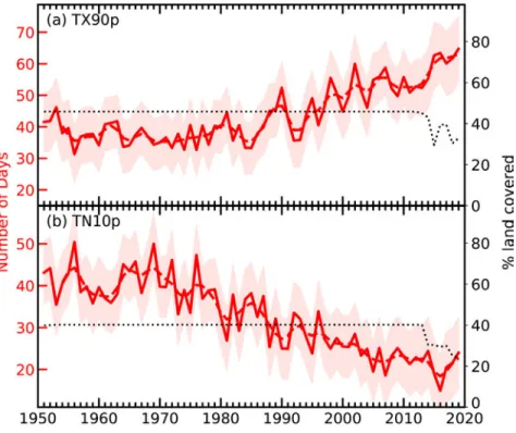
Over land, 2019 recorded the most number of warm days (TX90p, see Table 2.2 for definition) in the record dating to 1950, with over 60 days compared to the average of 36.5 (Fig. 2.4). The number of cool nights (TN10p) was low compared the last 70 years, but above average for the most recent decade. As the spatial coverage of the in situ GHCNDEX (Donat et al. 2013) dataset is not complete due to delayed or lack-ing report of up-to-date station data in many regions, the time series from the ERA5 reanaly-sis (Hersbach et al. 2020; Fig. 2.5; Fig. A2.5) is also shown. A similar picture emerges, but the number of warm days does not exceed the record maximum set in 2016. Similarly, the number of cool nights is also close behind the record minimum of 2016. Dif-ferences with GHCNDEX may be the result of the more complete coverage of ERA5.

The number of warm days is high over Europe and Austra-lia from GHCNDEX (Plate 2.1c), Table 2.2. WMO Expert Team on Climate Change Detection and Indices (ETCCDI; Zhang et al. 2011) temperature indices used in this section and their definitions.

Index Name Definition

TX90p Warm days Count of days where the maximum temperature was above the _{climatological 90th percentile (defined over 1961–90, days)} TN10p Cool nights Count of days where the minimum temperature was below the _{climatological 10th percentile (defined over 1961–90, days)}

TNx Maximum “night-time” _temperature Warmest minimum temperature (TN, °C) Fig. 2.4. Time series of (a) TX90p (warm days) and (b) TN10p (cool nights).

The red dashed line shows a binomial smoothed variation, and the shaded band the uncertainties arising because of incomplete spatio-temporal coverage estimated using ERA5 following Brohan et al. (2006). The dot-ted black line shows the percentage of land grid boxes with valid data in each year. (Source: GHCNDEX.)

(22)

S29

corresponding with the strong heat wave events in both these regions during 2019. In June large parts of Europe experienced daily maximum temperatures over 35°C, and France broke its national record with 46.0°C at Vérargues on the 28th. In July, France also sweltered under its record warm-est night (TNx), with a national average of 21.4°C on 24–25 July, and a new maximum temperature record of 42.6°C was set for Paris on the 25th. Many other nations also experienced temperatures over 40°C during this period, with na-tional station records broken in the United Kingdom (38.7°C), Germany (42.6°C), the Netherlands (40.7°C), Belgium (41.8°C), and Luxembourg (40.8°C). The World Meteorological Organization (WMO) declared the month of July 2019 tied as the hot-test on record for the globe (WMO

2019), based on ERA5 (Hersbach et al. 2020).

Australia experienced heat waves both early and late in the year. A prolonged and extensive heat wave affected much of the country from late December 2018 through January 2019. Records set include Adelaide’s hottest day on record at 46.6°C on 24 January (with new records also set at neighboring stations) and Canberra’s longest run of days above 40°C on four consecutive days (14–17 January 2019). The all-time national average maximum temperature record was set on 17 December 2019 at 41.9°C, 1.59°C above the 2013 record, and 2.09°C above average (1961–90). Janu-ary, March, and December 2019 were nationally the warmest on record for the respective months, with February, April, July, October, and November each among their respective 10 warmest. The most recent Australian heat wave in summer 2019/20 is presented in detail in Sidebar 7.6.

Heat waves also occurred in May and June in Japan, with a maximum temperature of 39.5°C (Saroma, Hokkaido) on 26 May (monthly record for this site), and also Pakistan (51.1°C Jacobabad on 1 June) and India with (50.8°C Churu, 2 June). In February, the United Kingdom experienced above-average temperatures with maxima of 21.2°C recorded in London on the 26th (monthly record), around 14°C above average. Extreme temperatures also occurred over South America in 2019. Overall, the continent observed its second-warmest year on record, with heat waves dur-ing January in Chile and southeastern Brazil contributdur-ing to the warmth. Santiago, Chile, set a new maximum temperature record of 38.3°C on 27 January. In North America, the state of Alaska experienced its warmest year on record. Please refer to the relevant sections in Chapter 7 for more regional temperature details.

GHCNDEX (Donat et al. 2013), a gridded dataset of ETCCDI (Expert Team on Climate Change Detection and Indices) extremes indices, was used to characterize the extreme temperatures over land. Indices are calculated from daily temperature values from the GHCND (Menne et al. 2012) and have been interpolated onto a 2.5° × 2.5° grid. As can be seen in Plates 2.1c,d, the spatial cov-erage is sparse, with available data for 2019 restricted to North America and parts of Eurasia and Australia. This lack of coverage arises both from gaps in the historical coverage (e.g., sub-Saharan

Fig. 2.5. Time series of (a) TX90p (warm days) and (b) TN10p (cool nights). The red dashed line shows a binomial smoothed variation. (Source: ERA5.)

(23)

S30

Africa) and also from delays in data transmission. ERA5 reanalysis (Hersbach et al. 2020) can be used to fill in some of these gaps, but because this dataset has a shorter temporal coverage, the reference period is necessarily different (1981–2010 compared to 1961–90 in GHCNDEX), which can lead to apparently different temporal behavior (Dunn et al. 2020).

Extreme heat, known as marine heat waves (MHWs), may enter the oceans through surface heat flux or advection. Satellite observations of SST can be used to monitor and categorize MHWs, as defined in Hobday et al. (2016, 2018). A category “I Moderate” MHW is defined as a period of time in which SST is above the 90th-percentile threshold of temperatures at a given location and day-of-year for five days or longer (Hobday et al. 2018). The MHW is categorized as “II Strong” if the largest temperature anomaly during the event is more than twice as large as the difference between the seasonally varying climatology and the 90th-percentile threshold. The MHW is “III Severe” if the largest anomaly is more than triple the difference, and “IV Extreme” if four times the difference or greater. Using NOAA OISST v2.1 (Banzon et al. 2020), the MHW category recorded most often in the ocean for 2019 was “II Strong” (41% of ocean surface), exceeding the lower category “I Moderate” (30%) for the sixth consecutive year (Fig. 2.6). Category “III Strong” MHWs (2%) were exceeded by “IV Extreme” MHWs (3%) for the fourth consecutive year. In total, 84% of the surface of the ocean experienced an MHW in 2019. There was an average of 74 MHW days per ocean pixel, an increase from 61 in 2018, but below the 2016 record of 83. The average daily MHW occurrence throughout the ocean was 20%, an increase over the 2018 average of 17%, and less than the 2016 record of 23%.

4) Tropospheric temperature—J.R. Christy, C. A. Mears, S. Po-Chedley, and L. Haimberger

The 2019 global lower tropospheric temperature (LTT), which encompasses the atmosphere from the surface to ~10 km, ranked second warmest in seven datasets and first or third in the remaining two (Fig. 2.7). These records extend back to 1958 using radiosonde (balloon-borne instrumentation) data and one reanalysis dataset (JRA55), which demonstrate reasonable agree-ment with the 40+ year satellite record (since late 1978) and two other reanalysis datasets (since 1979 and 1980, ERA5 and MERRA2, respectively). A weak El Niño contributed to increased global temperatures as 2019 values were +0.44° to +0.68°C higher than the 1981–2010 average (depend-ing on the dataset), be(depend-ing just slightly cooler (~0.07°C on average) than the record warm year of 2016. At least four of the five globally complete datasets (ERA5, MERRA2, JRA55, RSS, UAH) recorded each of the four months—June, September, November, and December—as experiencing their warmest monthly global LTT.

Fig. 2.6. Annual MHW occurrence using a climatology base period of 1982–2011. (a) Daily average percent of the ocean that experienced a MHW. (b) Total percent of the ocean that experienced a MHW at some point during the year. The values shown are for the highest category of MHW experienced. (c) Total average of daily MHW occurrence throughout the entire ocean. (Source: NOAA OISST.)

(24)

S31

The warming rate of the global tro-posphere since 1958, as the median of available datasets, is +0.18 (range +0.16 to +0.20) °C decade−1_{. The median}

warming rate since 1979 is also +0.18 (range +0.13 to +0.21) °C decade−1_{, which}

includes records derived from micro-wave satellite measurements (Table 2.3). Taking into consideration the temporary cooling due to volcanic aerosols caused by eruptions in 1982 and 1991, as well as the El Niño/La Niña cycle, there remains a global warming trend since 1979 of +0.12 ± 0.04°C decade−1_{unexplained by}

these ephemeral, natural phenomena (Christy and McNider 2017, updated and calculated using ERA5, RSS, and UAH datasets).

The spatial details of the departures of LTT from the 1981–2010 mean are depicted in Plate 2.1e as provided by the European Centre for Medium-Range Forecasts Reanalysis version 5 (ERA5). Above-average anomalies dominate the 2019 ERA5 map with negative regions occupying only 8.1% of the global surface area, including much of North America, a portion of South Asia, and midlati-tude regions of the south-ern oceans. These below-average LTTs comprise the third-smallest such area after 2016 and 2017.

Much higher-than-aver-age temperatures included several regions that expe-rienced record high tem-peratures relative to this 41-year period of observa-tions. Alaska, Greenland, central Europe, and south-ern Africa were especially warm. The broad warmth of the tropical belt is a typical signature of an El Niño year.

The warming trend may be depicted in a geographi-cal context by determining Table 2.3. Estimates of lower tropospheric temperature (LTT) and tropical

tropospheric temperature (TTT) decadal trends (°C decade−1_{) beginning in 1958}

and 1979 from the available datasets.

Area Global Global Tropical Tropical

Layer LTT LTT TTT TTT Start Year 1958 1979 1958 1979 Radiosonde NOAA/RATPACvA2 +0.18 +0.21 +0.16 +0.16 RAOBCOREv1.7 +0.18 +0.19 +0.15 +0.15 RICHv1.7 +0.20 +0.21 +0.19 +0.22 Satellite RSSv4.0 — +0.21 — +0.18 UAHv6.0 — +0.131 _— _+0.13 NOAA/STARv4.1 — — — +0.23 UWv1.0 — — — +0.17 Reanalyses ERA5 — +0.17 — +0.16 JRA-55 +0.16 +0.16 +0.16 +0.15 NASA/MERRA-22 _— _+0.17 _— _+0.16 Median +0.18 +0.18 +0.16 +0.16

1_{The UAH LTT weighting function is slightly different in order to reduce the impact of surface}

emissions and enhance the tropospheric signal, resulting in a global trend value typically cooler by 0.01°C decade−1_{relative to the standard LTT weighting function.}

2_{NASA/MERRA-2 begins in 1980.}

Fig. 2.7. Time series of global annual temperature anomalies (°C) for the lower troposphere from (a) radiosondes, (b) satellite microwave emissions, and (c) reanalyses.

(25)

S32

the year in which the extreme high (and low) annual values at each grid point occurred, then summing those areally-weighted grids by year. If all regions of Earth experienced a monotoni-cally increasing temperature, then each new year would see 100% of the global area achieving a record high temperature; however, if the global trend were zero over the 41-year period of record but characterized by random inter-annual variability, each year would experience, on average, an area of 2.4% of record high (or low) temperatures. With our climate system characterized by both an increasing trend and inter-annual variations since 1979, the area in 2019 of record high temperatures was 15.6% (calculated as the average of ERA5, RSS, and UAH). The stippling in Plate 2.1e identifies these grids (see also Fig. A2.6). Two years with major El Niño events, 1998 and 2016, recorded areal extents for the highest temperatures of 16.9% and 20.1%, respectively (no repeated records). Since 1979, the year with the largest coverage of record low annual-average temperatures was 1985 with 19.8% due in part to a concurrent La Niña event.

Global and tropical trends are listed in Table 2.3. When examining the time series of these three methods (radiosondes, satellites, reanalyses), the radiosondes display an increasing trend over the past 10 years relative to the other methods (see trend values in column Global LTT 1979 and Fig. A2.7) This may be related to a change in software installed after 2009 in many stations to improve the tropospheric humidity and temperature values (Christy et al. 2018).

The tropical (20°N–20°S) tropospheric temperature (TTT, surface to ~15 km) variations and trends are similar to those of the global values. The median TTT trends from the available da-tasets since 1958 and 1979 are both +0.16°C decade–1_{with ranges of +0.15 to +0.19 and +0.13 to}

+0.23°C decade–1_{, respectively (Table A2.1). This layer in the tropics is a key area of interest due}

to its expected significant response to forcing, including that of increasing greenhouse gas con-centrations (McKitrick and Christy 2018; see Fig. A2.8).

Radiosondes provide coverage wherever the stations exist. Considerable areas of the globe are thus not sampled, and this can lead to a misrepresentation of the global average. Satellites es-sentially observe the entire Earth each day, providing excellent geographic coverage, but whose radiances provide bulk-layer atmospheric measurements only. There are some key adjustments that are required too, and the methods adopted by different teams lead to the range in the results (Haimberger et al. 2012; Po-Chedley et al. 2015; Mears and Wentz 2016; see also Figs. A2.7 and A2.9). Full input reanalyses use essentially all available data, including radiosonde and satellite, ingested into a continuously updated global circulation model, thus providing full geographic and vertical coverage. Given the many differences in how the reanalyses are constructed from center to center, the consistency among their 41-year trends is encouraging.

5) Stratospheric temperature—W. J. Randel, C. Covey, and L. Polvani

Temperatures in the middle and upper stratosphere continued to decline to their lowest recorded values since 1979, i.e., the beginning of the satellite era. Lower stratosphere temperatures have been relatively constant since ~1998, with small interannual changes. The polar stratospheric regions were influenced by sudden stratospheric warming (SSW; Charlton and Polvani 2007) events in both hemispheres, in the Arctic in January 2019 and in the Antarctic in September 2019. The Antarctic event was highly unusual, being only the second SSW observed in the SH since 1979 (see Sidebar 6.1 for more details).

Time series of annual anomalies of middle and upper stratosphere temperatures from satellite observations are shown in Figs. 2.8a–c. These data represent ~20-km thick layer measurements from the Stratospheric Sounding Unit (SSU) merged with more recent satellite measurements (Randel et al. 2016; Zou and Qian 2016). Middle and upper stratospheric temperatures show distinctive cooling since 1979, with stronger negative trends at higher altitudes, which is a char-acteristic response to increases in atmospheric CO2 (Manabe and Wetherald 1967). The cooling is

modulated by upper stratospheric ozone changes, with somewhat weaker stratospheric cooling after 1998 tied to observed increases in ozone. The ozone is evolving as a response to changes