HAL Id: hal-01160831
https://hal.archives-ouvertes.fr/hal-01160831
Preprint submitted on 8 Jun 2015HAL is a multi-disciplinary open access archive for the deposit and dissemination of sci-entific research documents, whether they are pub-lished or not. The documents may come from teaching and research institutions in France or abroad, or from public or private research centers.
L’archive ouverte pluridisciplinaire HAL, est destinée au dépôt et à la diffusion de documents scientifiques de niveau recherche, publiés ou non, émanant des établissements d’enseignement et de recherche français ou étrangers, des laboratoires publics ou privés.
Distributed under a Creative Commons Attribution - NonCommercial| 4.0 International
Constrained Convex Neyman-Pearson Classification
Using an Outer Approximation Splitting Method
Michel Barlaud, Patrick Louis Combettes, Lionel Fillatre
To cite this version:
Michel Barlaud, Patrick Louis Combettes, Lionel Fillatre. Constrained Convex Neyman-Pearson Classification Using an Outer Approximation Splitting Method. 2015. �hal-01160831�
Constrained Convex Neyman-Pearson Classification Using an
Outer Approximation Splitting Method
Michel Barlaud, [email protected]
Laboratoire I3S 2000 Route des Lucioles 06903 Sophia Antipolis, France Patrick L. Combettes, [email protected]
Sorbonne Universit´es – UPMC Univ. Paris 06,
UMR 7598, Laboratoire Jacques-Louis Lions, F-75005 Paris, France Lionel Fillatre, [email protected]
Laboratoire I3S 2000 Route des Lucioles 06903 Sophia Antipolis, France June 8, 2015
Abstract
This paper presents an algorithm for Neyman-Pearson classification. While empirical risk min-imization approaches focus on minimizing a global risk, the Neyman-Pearson framework mini-mizes the type II risk under an upper bound constraint on the type I risk. Since the 0/1 loss function is not convex, optimization methods employ convex surrogates that lead to tractable minimization problems. As shown in recent work, statistical bounds can be derived to quantify the cost of using such surrogates instead of the exact 1/0 loss. However, no specific algorithm has yet been proposed to actually solve the resulting minimization problem numerically. The contribution of this paper is to propose an efficient splitting algorithm to address this issue. Our method alternates a gradient step on the objective surrogate risk and an approximate projection step onto the constraint set, which is implemented by means of an outer approximation subgra-dient projection algorithm. Experiments on both synthetic data and biological data show the efficiency of the proposed method.
Convex optimization, machine learning, calibrated risk, splitting algorithm
1
Introduction
Support Vector Machine (SVM) is a powerful and well-established method for machine learning [10;28]. Standard SVM methods use the hinge loss as a convex surrogate to the 0/1 loss. Generally speaking, the choice of the surrogate loss impacts significantly statistical properties [3]. When using the classical empirical risk minimization approach, the majority class is well classified, whereas the minority class is poorly classified. In many applications, however, the minority class is often the most relevant. For example, in biological applications, patients with pathology are of more interest although they constitute a minority class. Consequently, controlling false negative rates is of utmost importance in biomedical diagnosis.
The Neyman-Pearson is an alternative to the classical empirical risk minimization approach min-imizing a global classification risk consisting of a weighted sum of type I and type II risks. The Neyman-Pearson approach minimizes the type II risk subject to an upper bound on the type I risk. To the best of our knowledge, the only previous work dealing with constrained Neyman-Pearson framework was on statistical evaluation [7; 18; 24; 23; 27]. These approaches provide a quanti-tative relationship between the minimization of the empirical risk and the minimization of the 0/1 risk. However, they did not propose any algorithm for solving the numerical optimization problem, which consists of minimizing an empirical objective subject to an empirical constraint.
The present paper deals with binary classification. Our main contribution is to propose an im-plementable algorithm with guaranteed convergence for solving the Neyman-Pearson classification problem. Section 2 deals with state-of-the-art statistical results on Neyman-Pearson classification. Section 3 presents our new splitting algorithm. Finally, Section 4 presents experiments on both synthetic and real RNA-seq lung cancer data from the TGCA dataset.
2
Classification risk and classifiers
2.1 Empirical risk minimization
Henceforth, theRd-valued random vector X represents a feature vector, the{−1, 1}-valued ran-dom variable Y represents the associated label indicating to which class X belongs, and P denotes the underlying probability measure. A classifier is a mapping h : Rd 7→ [−1, 1], the sign of which
returns the predicted class given X. An error occurs when Yh(X) ⩽ 0. The classification risk associated with a classifier h is
R(h) = P[Yh(X)⩽ 0] = E(1]−∞,0](Yh(X))
)
, (1)
where 1]−∞,0] denotes the characteristic function of ]−∞, 0], i.e., the 0/1 loss function. The above
formulation leads in general to numerically intractable optimization problems and it must be sim-plified. In the present paper, we focus on linear classifiers, meaning that the function h is of the form
hw:Rd→ R: x 7→ ⟨x | w⟩ = x⊤w, (2)
for some weight vector w∈ Rd. In addition, we shall replace the nonconvex 0/1 loss function 1]−∞,0]
in (1) by a suitable convex surrogate, i.e., a convex function ϕ :R 7→ [0, +∞[ which approximates 1]−∞,0](see Fig.1). This leads to the surrogate risk
Rϕ(h) = E
(
ϕ(Yh(X)))= E(ϕ(Y⟨X | w⟩)). (3)
Our problem set-up is as follows. We assume that m annotated samples (xi)1⩽i⩽minRdare available,
resulting from the observation of independent realizations of the feature vector X. The associated realizations (yi)1⩽i⩽m of the label Y are variables valued in {−1, +1}, which represent the two
classes. The features (xi)1⩽i⩽m are problem-dependent, e.g., bag of word and Fisher vectors in
image classification, gene expression in biological application, etc. In the classical empirical risk minimization approach, the goal is to learn w by minimizing the surrogate empirical risk
φ : Rd→ R: w 7→ 1 m m ∑ i=1 ϕ(yi⟨xi | w⟩ ) . (4)
In the context of empirical risk minimization, Bartlett et al. [3] provide a general quantitative relationship between the risk using the 0/1 loss and the risk using a surrogate loss function ϕ :R → R. They show that this relationship gives upper bounds on the excess risk under the provision that the convex loss ϕ is calibrated, i.e., ϕ is differentiable at 0 with ϕ′(0) < 0.
2.2 Controlling false alarms
The type I risk associated with a classifier h onRdis
R−(h) = P(Yh(X)⩽ 0 | Y = −1), (5)
while the type II risk is defined by
R+(h) = P(Yh(X)⩽ 0 | Y = +1). (6)
The Neyman-Pearson classification consists in solving minimize
R−(h)⩽α
R+(h), (7)
where α ∈ ]0, 1[ is user-defined. Now, let us introduce the ϕ-type I risk and the ϕ-type II risk associated with a classifier h as
R−ϕ(h) = E(ϕ(Yh(X))| Y = −1) (8)
and
R+ϕ(h) = E(ϕ(Yh(X))| Y = +1), (9)
respectively. Let PY denote the conditional distribution of X given Y. We split the set of samples
(xi)1⩽i⩽minto the subset (x−i )1⩽i⩽m−of features which have distribution P−1, and the complemen-tary subset (x+i )1⩽i⩽m+ of features which have distribution P+1 (the sample sizes m− and m+ are
deterministic). The empirical surrogate ϕ-risks of a classifier h are defined by
b R−ϕ(h) = 1 m− m− ∑ i=1 ϕ(−h(x− i )) and Rb + ϕ(h) = 1 m+ m+ ∑ i=1 ϕ(h(x+i )). (10)
2.3 Constrained Neyman-Pearson framework
To process unbalanced datasets, classical methods rely on the weighted objective b
Rϕ,ρ= bR−ϕ + ρ bR+ϕ, (11)
where ρ controls the unbalanced dataset. An alternative is a cost-sensitive approach with Lagrangian formulation such as C-SVM or ν-SVM [12;29], where the parameter ν controls the trade-off between the two types of errors. Unfortunately, Lagrangian methods require cross validation for tuning the parameter ρ or ν. It is well known that this cross validation can lead to poor classification accuracy. To circumvent this issue, we propose the following constrained Neyman-Pearson calibrated classifi-cation approach. The Neyman-Pearson paradigm is an alternative to the empirical risk minimization
approach in statistical learning. It attempts to find a classifier ˜h as a solution to the constrained optimization problem minimize b R−ϕ(h)⩽τ b Rϕ+(h), (12)
where τ ∈ ]0, 1[ is chosen as a function of α in such a way that the relaxed constraint bR−ϕ(˜h) ⩽ τ
on the type I risk implies that the constraint R−(˜h) ⩽ α on the type I risk in (5) is satisfied by ˜
h with high probability. The statistical properties of ˜h are given in the following theorem initially established in [18] for aggregate classifiers and applied here to bounded linear classifiers. A bounded linear classifier is a special case of an aggregate classifier.
Let α ∈ ]0, 1[, let δ ∈ ]0, 1/2[, let H be the set of linear classifiers hw: x 7→ ⟨x | w⟩ such that
∥w∥1⩽ M for some fixed M ∈ ]0, +∞[, and set
Hα ϕ = { h∈ H R−ϕ(h)⩽ α}. (13) Set ε = inf{θ∈ ]0, 1[ Hθαϕ ̸= ∅} (14)
and let ϕ : R → R be a differentiable convex function with a β-Lipschitz derivative. Assume that there exists θ∈ ]0, 1[ such that Hθαϕ ̸= ∅. Set
γ = 4β √ 2 log ( 4d δ ) (15) and m0= inf { m∈ N m ⩾ ( 4γ α(1− ε) )2} , (16)
and suppose that there exists ξ ∈ R such that ∥X∥∞ ⩽ ξ almost surely. Assume that m− ⩾ m0 and
let ˜hbe a solution to (12), where τ = α− γ/√m−. Then, with probability at least 1− 2δ,
R−(˜h)⩽ Rϕ−(˜h)⩽ α (17) and R+ϕ(˜h)− inf h∈Hα ϕ Rϕ+(h)⩽ 4γ ϕ(1) (1−ε)α√m−+ 2γ √ m+. (18)
This theorem shows that the classifier ˜hobtained by minimizing the empirical surrogate ϕ-risk is a solution to (7). It also shows that the ϕ-type II risk of ˜htends to the minimum ϕ-type II risk over
Hα
ϕas min{m−, m+} becomes arbitrarily large. The convergence rate of the ϕ-type II risk is bounded
by (18).
2.4 Smooth calibrated loss
We restrict our attention to calibrated convex surrogate losses that satisfy the following properties [6].
Assumption 1 The loss ϕ : R → R is convex, everywhere differentiable with a Lipschitz-continuous gradient, and twice differentiable at 0 with ϕ′′(0) = max ϕ′′. Furthermore, there exists an increasing function f : R → [0, 1] which is antisymmetric with respect to the point (0, f(0)) = (0, 1/2) such that
(∀t ∈ R) ϕ(t) = −t +∫−∞t f (s)ds.
This interesting class of smooth calibrated losses [11], allows us to compute the posterior esti-mation without Platt estiesti-mation [17]. The function f maps directly a real-valued prediction h of a sample xi to a posterior estimation
P[Yi = +1|xi] = f (h(xi)) (19)
for the class +1. Now, in connection with (4), consider the convex function
φ+:Rd→ R: w 7→ 1 m+ m+ ∑ i=1 ϕ(⟨x+i | w⟩). (20)
Then, under Assumption1, φ+ is differentiable and its gradient
∇φ+: w7→ 1 m+ m+ ∑ i=1 ϕ′(⟨x+i | w⟩)x+i , (21)
has Lipschitz constant 1/β, where
β = m
+
ϕ′′(0)∑mi=1+∥x+i ∥2. (22)
Let us note that computer vision classification involves normalized high dimensional features such as Fisher vectors [21]. In this case, (22) reduces to
β = 1
ϕ′′(0). (23)
Examples of functions which satisfy Assumption1include that induced by f : t7→ 1/(1 + exp(−t)), which leads to the logistic loss
ϕ : t7→ ln(1 + exp(−t)), (24)
for which ϕ′′(0) = 0.25. Other examples are the calibrated version of the linear hinge loss
ϕ : t7→ max{0, −t} − ln(√2 +|t|) + ln(2), (25)
as well as the Matsusita loss [15]
ϕ : t7→ 1
2(−t + √
1 + t2). (26)
Note that the boosting exponential loss does not satisfy the above properties, and that neither does the hinge loss ϕ : t7→ max{1, −t} used in classical SVM.
R R 0 1 | 1
Figure 1: Convex surrogate functions for the 0/1 loss function 1]−∞,0](in red): the calibrated hinge
loss ϕ : t 7→ max(0, −t) + ln(2) − ln(√2 +|t|) (in orange), the logistic loss ϕ: t 7→ ln(1 + e−t) (in blue), and the Matsusita loss ϕ : t7→ (√t2+ 1− t)/2 (in magenta).
3
Splitting algorithm
3.1 General framework
In this section, we propose an algorithm for solving the Neyman-Pearson classification problem (12). This algorithm fits in the general category of forward-backward splitting methods, which have been popular since their introduction in signal processing and machine learning [9; 16; 22; 25]. These methods offer flexible implementation with guaranteed convergence of the sequence of iterates they generate, a key property to ensure the reliability of our variational classification scheme.
The minimization problem (12) can be recast as follows.
Problem 1 Suppose that ϕ satisfies Assumption1, define φ+as in (20), define
φ−:Rd→ R: w 7→ 1 m− m− ∑ i=1 ϕ(yi ⟨ x−i | w⟩), (27) and set C = { w∈ Rd φ−(w)⩽ τ } . (28) The problem is to minimize w∈C φ +(w). (29)
Let us note that for reasonably sized data set, φ+or φ−will be coercive and hence the Problem1
will have at least one solution [5, Proposition 11.14]. As noted in Section2.4, φ+is a differentiable
convex function and its gradient has Lipschitz constant 1/β, where β is given by (22). Likewise, since φ−is convex and continuous, C is a closed convex set. The principle of a splitting method is to use the constituents of the problems, here φ+ and C, separately [5]. In the problem at hand, it
is natural to use the projection-gradient method to solve (29). This method, which is an instance of the proximal forward-backward algorithm [5], alternates a gradient step on the objective φ+and
a projection step onto the constraint set C. Given w0 ∈ Rd, a sequence (γn)n∈N of strictly positive
parameters, and a sequence (an)n∈N inRdmodeling computational errors in the implementation of
the projection operator PC, it assumes the form
for n = 0, 1, . . . ⌊
vn= wn− γn∇φ+(wn)
wn+1= PCvn+ an.
(30)
In view of (21), (30) can be rewritten as
for n = 0, 1, . . . vn= wn− γn m+ m+ ∑ i=1 ϕ′(yi ⟨ x+i | w⟩)yix+i wn+1= PCvn+ an. (31)
We derive at once from [9, Theorem 3.4(i)] the following convergence result, which guarantees the convergence of the iterates.
Let w0 ∈ Rd, let (γn)n∈Nbe a sequence in ]0, +∞[, and let (an)n∈Rdbe a sequence inRdsuch that ∑
n∈N
∥an∥ < +∞, inf
n∈Nγn> 0, and supn∈Nγn< 2β. (32)
Then the sequence (wn)n∈Ngenerated by (31) converges to a solution to Problem1.
The implementation of (31) is straightforward except for the computation of PCvn. Indeed, C
is defined in (27) as the lower level set of a convex function, and no explicit formula exists for computing the projection onto such a set. Fortunately, Proposition 3.1asserts that PCvn does not
have to be computed exactly. We can therefore implement it approximately by performing a sufficient number of iterations of an efficient algorithm designed for computing the projection onto a lower level set of a convex function. Next, we describe such an algorithm, which is borrowed from [4] and proceeds by successive outer approximations generated by subgradient projections.
3.2 Projection algorithm
η ∈ R be such that D ={p∈ Rd f (p)⩽ η}̸= ∅. Iterate for k = 0, 1, . . . if f (pk)⩽ η ⌊terminate. pk+1/2 = pk+ η− f(pk) ∥∇f(pk)∥2∇f(pk ) χk = ⟨ p0− pk| pk− pk+1/2 ⟩ µk=∥p0− pk∥2 νk =∥pk− pk+1/2∥2 ρk= µkνk− χ2k if ρ⌊ k= 0and χk⩾ 0 pk+1= pk+1/2 if ρ⌊k> 0and χkνk⩾ ρk pk+1 = p0+ ( 1 +χk νk )( pk+1/2− pk ) if ρk> 0and χkνk< ρk pk+1 = pk+ νk ρk ( χk ( p0− pk ) +µk ( pk+1/2− pk )) (33)
Then either the algorithm terminates in a finite number of iterations at PDp0 or it generates an
infinite sequence (pk)k∈Nsuch that pk → PDp0.
The principle of the above algorithm is as follows (see Fig.2). At iteration k, if f (pk) ⩽ η, then
pk ∈ D and the algorithm terminates with pk= PDp0. Otherwise, one first computes the subgradient
projection pk+1/2= pk+ η− f(pk) ∥∇f(pk)∥2∇f(pk ) (34) of pkonto D. We have [4] D⊂ H(pk, pk+1/2) = { p∈ Rd ⟨p− pk+1/2 | pk− pk+1/2 ⟩ ⩽ 0}. (35)
The closed half-space H(p0, pk+1/2) serves as an outer approximation to D at iteration k. On the
other hand, by construction, we also have a second similar outer approximation, namely
D⊂ H(p0, pk) =
{
p∈ Rd ⟨p− pk| p0− pk⟩ ⩽ 0
}
. (36)
As a result, D⊂ H(p0, pk)∩ H(pk, pk+1/2). The update pk+1 is computed as the projection of p0onto
the outer approximation H(p0, pk)∩ H(pk, pk+1/2). This update can be expressed explicitly in terms
of the vectors pk− p0 and pk+1/2− pkas described above. This provides a convergent sequence the
limit of which is the projection of p0 onto D.
3.3 Practical implementation
We have observed that (33) yields in a few iterations to a point close to the exact projection of p0
We can therefore insert the subroutine (33) into (31) (with p0 = vn, f = φ−, and η = τ ) to evaluate
approximately PCvnby performing only Kniterations of it at iteration n. In this case, it follows from
(33) that (31) reduces to for n = 0, 1, . . . vn= wn− γn m+ m+ ∑ i=1 ϕ′(yi ⟨ x+i | wn ⟩) yix+i p0 = vn for k = 0, 1, . . . , Kn ηk= α− 1 m− m− ∑ i=1 ϕ(yi ⟨ x−i | pk ⟩) if ηk⩾ 0 ⌊terminate. uk= 1 m− m− ∑ i=1 ϕ′(yi ⟨ x−i | pk ⟩) yix−i pk+1/2= pk+ ηk ∥uk∥2 uk χk= ⟨ p0− pk| pk− pk+1/2 ⟩ µk =∥p0− pk∥2 νk=∥pk− pk+1/2∥2 ρk= µkνk− χ2k if ρ⌊ k = 0and χk⩾ 0 pk+1= pk+1/2 if ρ⌊k > 0and χkνk⩾ ρk pk+1= p0+ ( 1 +χk νk )( pk+1/2− pk ) if ρk > 0and χkνk< ρk pk+1= pk+ νk ρk ( χk ( p0− pk ) +µk ( pk+1/2− pk )) wn+1 = pKn. (37)
3.4 Convergence of the inner loop
The theory shows that we need perform only Kn inner iterations as long as can guarantee that
the approximation errors (∥an∥)n∈N form a summable sequence. Consider iteration k of (37). Then,
since D⊂ H(p0, pk)and pkis the projection of p0onto H(p0, pk), we have∥pk−PDp0∥ ⩽ ∥p0−PDp0∥.
Hence pk ∈ D ⇔ pk= PDp0, i.e., f (pk)⩽ η ⇔ pk= PDp0. Now suppose that, for every k, f (pk) > η
(otherwise we are done). By convexity, f is Lipschitz-continuous on compact sets [5, Corollary 8.32], and therefore there exists a constant ζ such that 0 < f (pk)−η = f(pk)−f(PDp0)⩽ ζ∥pk−PDp0∥ →
0. In addition, since in our case intD̸= ∅, using standard error bounds on convex inequalities [20], there exists a constant ξ such that∥pk−PDpk∥ ⩽ ξf(pk)−η. So we can approximate the order of the
D =
{
p
∈ R
df (p)
⩽ η
}
{
p
∈ R
df (p)
⩽ f(p
k)
}
p
kp
0•
•
•
p
k+1• p
k+1/2∇f(p
k)
H(p
k, p
k+1/2)
H(p
0, p
k)
Figure 2: A generic iteration of (33) for computing the projection of p0 onto D. At iteration k,
the current iterate is pk and D is contained in the half-space H(p0, pk) onto which pk is the
pro-jection of p0 (see (36)). If f (pk) > η, the gradient vector ∇f(pk) is normal to the lower level set
{
p∈ Rd f (p)⩽ f(pk)
}
, and the subgradient projection pk+1/2of pkonto D is defined by (34); it is
the projection of pk onto the half-space H(pk, pk+1/2)of (35), which contains D. The update pk+1is
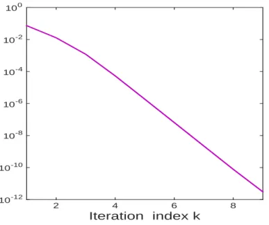
Iteration index k 2 4 6 8
f(p
k)-η
10-12 10-10 10-8 10-6 10-4 10-2 100Figure 3: Convergence of the projection inner loop.
such an analysis to be superfluous as the inner loop converges extremely fast and typically (Fig.3)
f (pk)− η ⩽ 10−12after just k = 9 iterations. So we have taken Kn= 9in our experiments.
4
Experimental evaluation
4.1 Setting
Classification and risk prediction based on gene transcription factor and clinical data sets in cancer analysis is currently a challenging task. Since the early classification work of [13;14] using DNA microarray data sets, state of the art classification methods have been based on empirical risk minimization approaches such as support vector machines; see the recent review [26] on feature selection for classification for more details. To the best of our knowledge no alternate optimization algorithm has been proposed for solving the constrained Neyman-Pearson classification Problem1. For this reason, we cannot perform comparisons in this experimental study.
In all experiments we use the logistic loss (24) as a surrogate. We use half of the data for training and half for testing, and we set α = 0.1. In the figures, we plot the 0/1 risk and surrogate risks or the classical global and mean accuracy as a function of the number of iterations of (37). We show in Fig.4a typical convergence pattern of (37).
Iteration number n 0 1000 2000 3000 4000 5000 Norm(W n -W ∞ ) 0 0.01 0.02 0.03 0.04 0.05 0.06 0.07 0.08 0.09 0.1
Figure 4: A typical convergence pattern for (37).
4.2 RNA-seq model and preprocessing
RNAseq is a recent high-throughput sequencing technology.1 The distribution model of RNA-seq is different from DNA microarray data and requires adapted preprocessing. The underlying distribution model of RNAseq is a negative binomial distribution [19]. Let Xij denote the observed
raw read count for gene i and library j, where 1 ⩽ i ⩽ p and 1 ⩽ j ⩽ the count Xij follows a
negative binomial distribution where mij is the mean and ψiis the dispersion for gene i. The mean
satisfies
mij = µiLiDj, (38)
where Li is the length of gene i, Dj is proportional to the total number of reads for library j (also
called the sequencing depth), and µi is the true and unknown expression level for gene i. We
propose to use a simple transformation, known to have an optimum property (i.e., to be the best of that degree of complexity) for mij large and ψi ⩾ 1 (see details in [2])
Zij = ln ( Xij + 1 2ψi ) . (39)
The transformation (39) makes the distribution of Zij closer to a monovariate normal distribution.
Its variance is approximately Ψ′(ψi), where Ψ′(t)denotes the second derivative of ln Γ(t) with respect
to t. The mean of Zij is approximately given by [2]
E(Zij) ≈ ln µi+ ln Li+ ln Dj− 1 2ψi + ln ( 1 + ψi 2mij ) . (40)
The last term in (40) is negligible when ψi≪ mij.
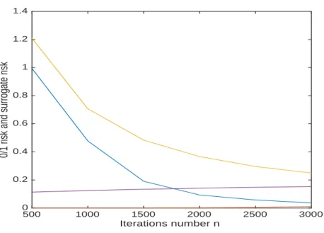
Iterations number n
500 1000 1500 2000 2500 3000
0/1 risk and surrogate risk
0 0.2 0.4 0.6 0.8 1 1.2 1.4
Figure 5: Synthetic data, training, 0/1 risk type I (in orange) and type I surrogate risk (in magenta) 0/1risk type II (in blue) and type II surrogate risk (in yellow).
4.3 Results on a synthetic dataset
We have generated artificial negative binomial samples for the counts Xij with 1000 genes for
each patient. We have 3340 patients in the first class and only 1040 patients in the minority class. The length Li of each gene is known and ψi = 6 for each gene i. The sequencing depths Dj are
generated as realizations of a Gaussian variable modelling the experimental variability. For the first class, the µi’s are chosen arbitrarily. The choice is based on typical values estimated from real
RNAseq measurements. For the second class, 20% of the µi’s (randomly chosen) of the first class are
changed: their values are increased or decreased randomly, by using Gaussian distributed offsets. The random nature of the Dj’s has no impact on classification. Finally, the counts Xij are generated
by using a negative binomial random generator. We then applied the transformation (39) to obtain the observations Zij.
The challenge is to predict whether an artificial patient belongs to one class or the other. The data set is unbalanced since we have 3340 samples in one class and only 1040 samples in the minority class consider as type I. We display in Fig. 5the performance of the algorithm in the training set. In this experiment, the projection algorithm requires only Kn = 9 iterations (which is typical). In
addition, the surrogate type I risk (in magenta) is perfectly controlled and induces a type I risk (in orange ) close to zero with the inequalities
R−(˜h)⩽ R−ϕ(˜h)⩽ α. (41)
This means that the statistical upper bound from [18] is overdetermined. Furthermore the estimated type II risk (in blue) is less than the type II surrogate risk (in yellow) as
Iterations number n
500 1000 1500 2000 2500 3000
0/1 risk and surrogate risk
0 0.2 0.4 0.6 0.8 1 1.2 1.4
Figure 6: Synthetic data, testing, 0/1 risk type I (in orange) and type I surrogate risk (in magenta), 0/1risk type II (in blue) and type II surrogate risk (in yellow).
We have similar results in the test set. Fig.6shows the performance of the algorithm in the test set. It can be noted that the constraint on the type I surrogate risk (in magenta) induces a type I risk (in orange) close to zero.
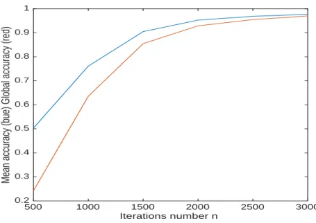
Fig.7shows the classical accuracy evaluation: mean accuracy (blue), and global accuracy (red).
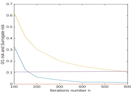
4.4 Results on the lung cancer RNAseq TCGA dataset
In this real experiment, we use the lung cancer RNAseq data set from the TGCA dataset (The Cancer Genome Atlas) [1]. The data set is highly unbalanced since we have 452 tumoral samples and only 58 samples without tumor. The goal is to predict from the RNAseq dataset whether there is a tumor or not. We use a classical filtering method for a coarse gene selection [13], [14], where the score
Si = |µ + i − µ−i |
σ+i + σi− (43)
is close to the Fisher score, and µi is the mean and σi the standard deviation in each class. Fig.8
shows the performance of the algorithm in the test set. Similarly to experiment on synthetic data set, It can be noted that the constraint on the type I surrogate risk (in magenta) induces a type I risk (in orange) close to zero.
Fig. 9 shows the performance of the algorithm for the test set. The constraint on the type I surrogate risk (in magenta), induces a type I risk (in orange) close to zero. The estimated type II risk (in blue) is smaller than the type II surrogate risk (in yellow).
Iterations number n
500 1000 1500 2000 2500 3000
Mean accuracy (bue) Global accuracy (red)
0.2 0.3 0.4 0.5 0.6 0.7 0.8 0.9 1
Figure 7: Synthetic data, testing, global (in blue) and mean (in red) accuracy.
Iterations number n
100 200 300 400 500 600
O/1 risk and surrogate risk
0 0.1 0.2 0.3 0.4 0.5 0.6 0.7
Figure 8: Tumor, training, 0/1 risk type I (in orange) and type I surrogate risk (in magenta) 0/1 risk type II (in blue) and type II surrogate risk (in yellow).
Iterations number n
100 200 300 400 500 600
0/1 risk and Surrogate risk
0 0.1 0.2 0.3 0.4 0.5 0.6 0.7
Figure 9: Tumor, Testing, 0/1 risk type I (in orange) and type I surrogate risk (in magenta) 0/1 risk type II (in blue) and type II surrogate risk (in yellow).
Iterations number n
100 200 300 400 500 600
Mean accuracy (blue) Global accuracy (red)
0.7 0.75 0.8 0.85 0.9 0.95 1
An extensive study on lung cancer data set using our new algorithm is currently being evaluated by colleagues in biology.
5
Conclusion and future work
We have proposed an efficient algorithm to solve the Neyman-Pearson classification problem. Assuming that the surrogate loss is smooth with a Lipschitz gradient, we have provided a new algo-rithm which alternates a gradient step on the objective surrogate loss and an approximate projection step onto the constraint set. Let us note that we have presented Proposition3.2(and, therefore, al-gorithm (37)) with a single constraint. However, the results of [4; 8] allow for the use of several constraints (each is then activated by its own subgradient projector). Thus, additional information about the problem can be easily be injected in (29), in particular in the form of constraints on w. This will be explored elsewhere. Experiments on both synthetic data and biological data show the ef-ficiency of our new method. On-going work includes joint feature selection (such as DNA mutations) and classification for the Neyman-Pearson classification problem.
6
Appendix: Proof of Theorem
2.3
SetBM =
{
w∈ Rd ∥w∥1⩽ M
}
and let{ei}1⩽i⩽d be the canonical basis ofRd. ThenBM is the
convex hull of the set
S ={si}1⩽i⩽2d={±Mei}1⩽i⩽d, (44)
where si = M ei for 1⩽ i ⩽ d and si =−Mei−dfor d + 1⩽ i ⩽ 2d. Hence, for every w ∈ BM, there
exists (λwi )1⩽i⩽2d∈ [0, +∞[2dsuch that
∑2d i=1λwi = 1and w = 2d ∑ i=1 λwi si. (45)
It follows that the associated bounded linear classifier hwis
hw: x7→ ⟨x | w⟩ = 2d
∑
i=1
λwi ⟨x | si⟩. (46)
Let us note that ( ∀x = (xi)1⩽i⩽d ∈ Rd ) ⟨x | si⟩ = { M xi if i∈ {1, . . . , d}, −Mxi−d if i∈ {d + 1, . . . , 2d}. (47)
Under the assumption that∥X∥∞⩽ ξ a.s., it follows that, without any loss of generality, the feature vector X can be normalized so that∥X∥∞ ⩽ 1 a.s. Hence ⟨· | si⟩: Rd 7→ [−1, 1]. As shown in [18,
Theorem 5], a classifier which is a convex combination of base classifiers fromRdto [−1, 1] satisfies the properties given in Theorem2.3. According to (46), a bounded linear classifier hw is a convex
combination of the base classifiers (⟨· | si⟩)1⩽i⩽2d and hence a bounded linear classifier satisfies the
References
[1] https://tcga-data.nci.nih.gov/tcga/tcgaHome2.jsp
[2] F. J. Anscombe. The transformation of Poisson, binomial and negative-binomial data.
Biometrika, 35:246–254, 1948.
[3] P. L. Bartlett, M. I. Jordan, and J. D. McAuliffe. Convexity, classification, and risk bounds.
Journal of the American Statistical Association, 101:138–156, 2006.
[4] H. H. Bauschke and P. L. Combettes. A weak-to-strong convergence principle for Fej´ er-monotone methods in Hilbert spaces. Mathematics of Operations Research, 26:248–264, 2001. [5] H. H. Bauschke and P. L. Combettes. Convex Analysis and Monotone Operator Theory in Hilbert
Spaces. Springer, New York, 2011.
[6] W. BelHajAli, R . Nock, and M. Barlaud. Minimizing calibrated loss using stochastic low-rank newton descent for large scale image classification. In International Conference on Pattern
Recognition, 2014.
[7] A. Cannon, J. Howse, D. Hush, and C. Scovel. Learning with the Neyman-Pearson and min-max criteria. Technical report, Los Alamos National Laboratory, 2002.
[8] P. L. Combettes. Strong convergence of block-iterative outer approximation methods for convex optimization. SIAM Journal on Control and Optimization, 38:538–565, 2000.
[9] P. L. Combettes and V. R. Wajs. Signal recovery by proximal forward-backward splitting.
Mul-tiscale Modeling and Simulation, 4:1168–1200, 2005.
[10] N. Cristianini and J. Shawe-Taylor. An Introduction to Support Vector Machines and Other
Kernel-Based Learning Methods. Cambridge University Press, New York, 2000.
[11] R. D’Ambrosio, R. Nock, W. Bel Haj Ali, F. Nielsen, and M. Barlaud. Boosting nearest neighbors for the efficient estimation of posteriors. In European Conference on Machine Learning ’12, 2012. [12] M. A. Davenport, R. G. Baraniuk, and C. Scott. Tuning support vector machines for minimax and Neyman-Pearson classification. IEEE Transactions on Pattern Analysis and Machine
Intelli-gence, 32:1888–1898, 2010.
[13] T. S. Furey, N. Cristianini, N. Duffy, D. W. Bednarski, M. Schummer, and D. Haussler. Sup-port vector machine classification and validation of cancer tissue samples using microarray expression data. Bioinformatics, 16:906–914, 2000.
[14] I. Guyon, J. Weston, S. Barnhill, W. Vapnik, and N. Cristianini. Gene selection for cancer clas-sification using support vector machines. In Machine Learning, pp. 389–422, 2002.
[15] K Matsusita. Distance and decision rules. Annals of the Institute of Statistical Mathematics, 16:305–315, 1964.
[16] S. Mosci, L. Rosasco, S. Matteo, A. Verri, and S. Villa. Solving structured sparsity regularization with proximal methods. In Machine Learning and Knowledge Discovery in Databases, vol. 6322, pp. 418–433, 2010.
[17] J. C. Platt. Probabilistic outputs for support vector machines and comparisons to regularized likelihood methods. In Advances in Large Margin Classifiers, pp. 61–74. MIT Press, 1999. [18] P. Rigollet and X. Tong. Neyman-Pearson classification, convexity and stochastic constraints.
Journal of Machine Learning Research, 12:2831–2855, 2011.
[19] M. D. Robinson and A. Oshlack. A scaling normalization method for differential expression analysis of rna-seq data. Genome Biology, 11:R25, 2010.
[20] S. M. Robinson. An application of error bounds for convex programming in a linear space.
SIAM Journal on Control, 13:271–273, 1975.
[21] J. S´anchez, F. Perronnin, T. Mensink, and J. Verbeek. Image classification with the Fisher vector: Theory and practice. International Journal of Computer Vision, 105:222–245, 2013. [22] M. Schmidt, N. L. Roux, and F. R. Bach. Convergence rates of inexact proximal-gradient
meth-ods for convex optimization. In Advances in Neural Information Processing Systems 24, pp. 1458–1466. 2011.
[23] C. Scott. Performance measures for Neyman-Pearson classification. IEEE Transactions on
Infor-mation Theory, 53:2852–2863, 2007.
[24] C. Scott and R. Nowak. A Neyman-Pearson approach to statistical learning. IEEE Transactions
on Information Theory, 51:3806–3819, 2005.
[25] S. Sra, S. Nowozin, and S. J. Wright (eds.). Optimization for Machine Learning. MIT Press, Cambridge, MA, 2011.
[26] J. Tang, S. Alelyani, and H. Liu. Feature selection for classification: A review. Data
Classifica-tion: Algorithms and Applications. C. Aggarwal (ed.), CRC Press, 2014.
[27] X. Tong. A plug-in approach to Neyman-Pearson classification. Journal of Machine Learning
Research, 14:3011–3040, 2013.
[28] V. Vapnik. Statistical Learning Theory. John Wiley, New York, 1998.
[29] K. Veropoulos, C. Campbell, and N. Cristianini. Controlling the sensitivity of support vector machines. In Proceedings of the International Joint Conference on AI, pages 55–60, 1999.
![Figure 1: Convex surrogate functions for the 0/1 loss function 1 ] −∞ ,0] (in red): the calibrated hinge loss ϕ: t 7→ max(0, − t) + ln(2) − ln( √](https://thumb-eu.123doks.com/thumbv2/123doknet/12960048.376701/7.918.344.668.212.439/figure-convex-surrogate-functions-loss-function-calibrated-hinge.webp)