Borehold resistivity inversion

Borehole Resistivity Inversion

by

Yulia V. Garipova

Submitted to the Department of Earth, Atmospheric, and Planetary Sciences

in partial fulfillment of the requirements for the degree of

Master of Science

in Earth and Planetary Sciences

at the

MASSACHUSETTS INSTITUTE OF TECHNOLOGY

June 1997

MASSACHUSETTS

@ 1997

INSTITUTE OF TECHNOLOGY

Signature of Author ...

Department of Earth

,"

Certified by ...

Professorqrank Dale Morgan Thesis Advisor

Accepted by... .. .- ... ... .. ... Professor Thomas H. Jordan

Department Chair

MIT

LERAFES

Borehole Resistivity Inversion

Yulia V. Garipova

Submitted to the Department of Earth, Atmospheric, and Planetary Sci-ences on April 15, 1997, in partial fulfillment of the requirements for the

degree of Master of Science

Abstract

In this thesis we develop a procedure for performing the inversion of borehole resistivity data using the software package developed by Western Atlas Logging Services, Houston, TX. Direct current resistivity methods, namely lateral sounding and conventional laterolog methods, are the main interest in this thesis. In resistive formations drilled with a conductive mud, where induction methods are not logged, it becomes imperative to combine these two methods in order to provide a reliable solution to the inversion problem. Lateral sounding provides comprehensive informa-tion about the resistivity distribuinforma-tion away from the borehole, while the higher resoluinforma-tion of the laterolog allows for detailed delineation of the formation.

Computationally, the inversion is performed using the constrained least-squares Marquardt algo-rithm combined with singular value decomposition. The nonlinear inversion problem is linearized after each iteration of the Marquardt method. One of the main benefits of the algorithm is its abil-ity to incorporate all resistivabil-ity/conductivabil-ity methods into a unique solution that is able to explain and satisfy all measurements. Several levels of inversion analysis are considered, from one-dimensional inversion to a rigorous and comprehensive one-dimensional approach. With the two-dimensional approach, the data need not be corrected for borehole and shoulder bed effects. We demonstrate the method with multiple synthetic examples in which the algorithm successfully recovers the formation parameters. Different noise levels, resistivity contrasts, depths of invasion, and initial guesses are considered. The method is then applied to field data consisting of lateral sounding logs and laterologs. The inversion results provide the resistivity variation away from the borehole. In most cases, the true to invaded zone resistivity ratio and the depth of invasion clearly indicate the layers with the best reservoir properties. In general, the field data inversion results agree very well with the available perforation data.

Thesis Supervisor: Frank Dale Morgan Title: Professor, Earth Resources Laboratory

Acknowledgments

I would first like to thank my "co-advisors," Professors M. Nafi Toksoz and F. Dale Morgan, Nafi for bringing me to MIT and letting me stay a "logging alien" at ERL, and Dale for guiding me through the last two semesters. I have greatly benefited from my discussions with Dale, as well as appreciating his insight into different problems.

Second, I wish to thank the Western Atlas people for all the help and support they have provided during my two summers in Houston and with my thesis. They have contributed to ERL the eXpress software system which made this thesis possible, as well as given me an enormous amount of help with all my software and hardware problems. I am especially grateful to Kurt-M. Strack, Alberto Mezzatesta, Michael Frenkel, Lev Tabarovsky, Gregory Itskovich, Michael Jervis, D. J. Meredith, Ingo Geldmacher and many others.

The other important part of my thesis--the field data--comes from the Central Geophysical Expe-dition in Moscow, Russia, and I would like to thank Alexey S. Kashik for generously contributing the data. I am also endlessly grateful to my sister, Galina, who had put a lot of effort and time into handling everything for me in Moscow.

I wish to extend my gratitude to my officemates, Tony and Maria, for all the programming-com-puter-Spanish stuff I have learned from them, and to my ERL colleagues and staff: Sue Turbak, Liz Henderson, Jane Maloof, and Naida Buckingham.

Finally, I must thank the people who have always been there for me whenever I needed them: my parents, Valery and Valentina, my sister and her family, and my friend Constantin. I am also indebted to Axel Sigmar and his family for their support and friendship. After all, it was he who triggered my decision to come to MIT three years ago, which, for better or worse, has changed my entire life.

Table of Contents

A bstract ...

Acknowledgm ents ... Table of contents ... 1 Introduction ... 2 Borehole resistivity logging ...

2.1 Earth model parametrization ... 2.2 Borehole resistivity sounding ... Apparent resistivity concept ... Lateral sounding...

Theoretical responses: lateral sondes ...

Theoretical responses: normal sondes ...

Effect of formation parameters on lateral theoretical responses ... 2.3 L aterolog ...

2.4 Sum m ary ...

3 Forward model and inversion algorithm ...

3.1 General considerations ... 3.2 Forward modeling principles ... 3.3 Inverse problem ... G eneral concepts ... Logarithm ic rescaling ... Singular value decomposition

3.4 Employed inversion techniques

Least-squares inversion. Gauss-Newton algorithm

W eighted least-squares ...

Regularization methods. Marquardt algorithm ... Method of steepest descent

Singular value decomposition ... Introduction of constraints ... 3.5 Sum m ary ... 4 Synthetic data inversion ... 4.1 Earth model parameters ... 4.2 Sam pling rates ... 4.3 Initial guesses ...

4.4 Inversion results 4.5 Summary

5 Field data inversion

5.1 Types of inversion analyses

5.2 Data description and preprocessing 5.3 Layer boundaries detection

5.4 Depth matching

5.5 Mud resistivity adjustment 5.6 Field data inversion

Field example 1 Field example 2 Field example 3 6 Conclusions References ... 6 8 ... 8 8 ... 89 ... 89 ... 90 ... 9 2 ...9 3 ... 9 4 ... ...94 ...94 ...9 9 ... ... 10 3 ... 10 8 . . . 1 10

Chapter 1

Introduction

Rock resistivity is one of the most important logging measurements because it is generally a func-tion of rock porosity and the resistivity of the fluid occupying the pore space, the key rock proper-ties in the search for hydrocarbons. Modern logging technologies allow for the recording of enormous amounts of data, which generally leads to accurate analysis of formation properties. In practice, resistivity measurements typically provide apparent values of the formation resistivities associated with particular formation volumes that depend on the characteristics of the measure-ment devices. These apparent values depend on the variation of physical and/or geological charac-teristics of the surrounding formations. When interpreting the data, one usually defines an earth

model, which is a simplified earth structure described by a number of parameters, in our case,

layer thicknesses and resistivities. The interpretation of the data consists of extracting the infor-mation from the apparent resistivities to derive the actual forinfor-mation parameters.

One of the earliest methods for borehole resistivity data interpretation is the use of conven-tional correction charts. The correction charts represent the dependences and relationships among different earth model parameters. Various assumptions, such as layer boundary positions or the presence of drilling mud invasion in each layer, have to be made prior to interpretation. With chart interpretation, one usually attempts to introduce various corrections to the data, i.e. to exclude the influence of certain parameters on the tool response, and afterwards to determine the rest of the parameters. Therefore, correction charts rely heavily on the log analyst's experience, consume much time, and most importantly, rarely provide accurate and comprehensive information which would combine and explain all measurements. Faster and more powerful data processing and interpretation techniques, such as inversion, are necessary for extracting the required information from such large data collections.

Geophysical inversion attempts to find the best fitting earth model for the field data by mini-mizing the misfit (error) between the data and the theoretical responses obtained by forward mod-eling. In nonlinear problems, we start with defining the initial set of parameters (initial guess) for which the theoretical tool responses are linearized in the vicinity of the model. A parameter

change is calculated in order to reduce the difference between the measured data and the theoreti-cal response. If this difference can be further decreased by varying the parameters, the procedure is repeated iteratively until the algorithm converges to a solution. Convergence means that the misfit cannot be further reduced by changing the parameter vector. The obtained solution is not necessarily the correct one because local minima of the misfit function may exist. However, in many cases such minima can be avoided by using robust algorithms and choosing an appropriate initial guess and parameter constraints based on the "physical meaningness" of the solution for a particular problem.

Inversion techniques to solve for parameters of underground formations have been used in surface geophysics for many years. Inversion has been applied in borehole resistivity more recently. In 1984, Yang and Ward introduced the inversion of borehole normal resistivity logs via ridge regression. Their earth model is horizontally layered with radially homogeneous and isotro-pic layers and no borehole effect, which allows the use of the analytical solution for the potential distribution of a point source in an arbitrary layer. Thus, Yang and Ward's earth model is one-dimensional and has no vertical boundaries. Other studies on the ID inversion of borehole resis-tivity data include Dyos (1987), Spalburg (1989), Wallase et al. (1991).

Whitman et al. (1989, 1990) introduced a more complex model which accounted for the bore-hole effect and zones saturated with borebore-hole fluid (the invaded zones). They used the finite differ-ence approximation approach on an exponentially expanding grid in both vertical and horizontal directions. Therefore, the accuracy of the results is largely determined by the rate of grid expan-sion. Whitman (1989) considered both normal and lateral logs; however, each of the logs is treated separately. However, if the data recorded with different tools are treated and inverted sepa-rately, we may have as many solutions (earth models) for the inversion problem as there are mea-surements. Ultimately we would like to combine and invert all measurements simultaneously, providing for an improved solution.

In 1994, Mezzatesta et al. (Western Atlas Logging Services) introduced a two-dimensional

joint inversion of borehole resistivity measurements using the Marquardt algorithm combined

with singular value decomposition. With the joint inversion approach, one can simultaneously invert as many logs as there are available and hence satisfy and explain all resistivity measure-ments at once. In other words, the algorithm provides the means for integrating all available resis-tivity methods regardless of their physical principles.

Perhaps one of the main advantages of the algorithm developed by Western Atlas Logging Services is its "comprehensiveness" in terms of the number of tools and measurements that can be used in the inversion. The incorporation of normal and lateral resistivity devices into the software have allowed us to apply an entirely new approach in dealing with electrical logging data.

Normal and lateral logs are widely and successfully applied in Russia; moreover, some West-ern companies have recently made attempts to make use of the latest technologies and develop-ments and revive nonfocused logging (Vallinga and Yuratich, 1993). Considering the growing need in the industry for processing and interpreting nonfocused borehole resistivity data, this the-sis is devoted to the solution of the inverse problem for lateral rethe-sistivity sounding. The joint inversion software, along with the eXpressTM system, has been generously provided to us for this project by Western Atlas.

With lateral sounding, we have several resistivity measurements providing different vertical and radial resolutions. Each measurement is to a certain extent affected by the presence of the borehole fluid and in some cases by its penetration into the formation, as well as by the so called shoulder effect, which results from the finite layer thickness. The integration of these measurements allows us to yield a single distribution of resistivities away from the borehole consistent with all measurements. The inversion process enables the tool behavior to be simulated and simultaneously accounts for the borehole, invasion and shoulder effects.

The depth of investigation of any resistivity tool is largely defined by the tool geometry, especially by the spacing between the receiving and transmitting electrodes. Therefore, in a set of resistivity measurements with different depths of investigation, the shallower measurements are considered to be influenced mostly by the zones near the borehole wall, while the deeper measurements reflect the apparent resistivity far from the borehole. This means that, in a layer invaded with the drilling mud, shallow devices provide the apparent resistivity closest to the invaded zone resistivity. The deepest measurements will sample the resistivity of the uncontaminated part of the formation. Figures 1-1 through 1-5 show the results of the inversion of five resistivity logs with different depths of investigation (lateral sounding logs). A simple three-layer model was used to simulate and invert the synthetic data. Only the middle layer is invaded (depth of invasion Lxo = 1 m), with the invaded zone resistivity of 5 ohm-m and true resistivity of 100 ohm-m. The upper and lower layer resistivities are 3 ohm-m, and the mud is 1 ohm-m with a borehole diameter of 0.2 m.

Figure 1-1. Results of separate inversion of the lateral sounding log: L 0.45. (Synthetic and theo-retical curves overlap.)

U Model Lxo Rm 0 1.0 I.25 (m) (ohm-m) Inverted Lxo (m) i ive -te L co ..,.v. . .. 0.2 hodel Rt 200 10.2 Model Rt 200, (ohm-m) (ohm-m)

hodel Rxo Model Rxo

0.2 200 0.2 200 (ohm-m) (ohm-m) RXO from L 0.45 L 0.45 0.2 200 0.2 200 (ohm-m) (ohm-m) RT from L 0.45 Theor. L 0.45 0.2 200 0.2 200 (ohm-m) (ohm-m)

Figure 1-2. Results of separate inversion of the lateral sounding log: L 1.05. Model Lxo 0 1.25 (m) (ohm-m) Inverted Lxo 0 1 (m) Model Rt 0.2 200 0.2 Model Rt 2001 (ohm-m) (ohm-m)

Model Rxo hodel Rxo

0.2 200 0.2 200 (ohm-m) (ohm-m) RXO from L 1.05 (ohm-m) (ohm-m) RT from L 1.05 Theor. L 1.05 0.2 200 0.2 200 (ohm-m) (ohm-m) t

tec

1

1.0

Figure 1-3. Results of separate inversion of the lateral sounding log: L 2.25. U V Model Lxo 1 .0 1.25 (m) (ohm-m) Inverted Lxo 0 I (m) in er ed Lx -

pd-;::---

Hodel Rxo hodel Rxo

0.2 200 0.2 200 (ohm-m) (ohm-m) RXO from L 2.25 L 2.25 0.2 200 0.2 200 (ohm-m) (ohm-m) RT from L 2.25 Theor. L 2.25 0.2 200 0.2 200 (ohm-m) (ohm-m)

1

1.

INe

i

l

I[IILI

ll

LII

I

II

IIIi

n

5I

l

il

i

l

Figure 1-4. Results of separate inversion of the lateral sounding log: L 4.25. 0.2 Model Rt 200 10.2 Model Rt 200 (ohm-m) (ohm-m)

Model Rxo Model Rxo

0.2 200 0.2 200 (ohm-m) (ohm-m) RXO from L 4.25 L 4.25 0.2 200 0.2 200 (ohm-m) (ohm-m) RT from L 4.25 Theor. L 4.25 0.2 200 0.2 200 (ohm-m) (ohm-m) elmi

Figure 1-5. Results of separate inversion of the lateral sounding log: L 8.50. INUADED ZONE Model Lxo Rm 0 1..0 1.25 (m) (ohm-m) Inverted Lxo (m) in erted x Lxo Model Rt .0.2 200 Model Rt 200 (ohm-m) (ohm-m)

Model Rxo Model Rxo

0.2 200 0.2 200 (ohm-m) (ohm-m) RXO from L 8.50 L 8.5 0.2 200 0.2 200 (ohm-m) (ohm-m) RT from L 8.50 Theor. L 8.50 0.2 200 0.2 200 (ohm-m) (ohm-m) in ett

Figure 1-1 shows the inversion results for the shallowest measurement (L 0.45); the size of the device (and hence the depth of investigation) increases from Figure 1-1 to 1-5. The leftmost tracks in Figures 1-1 - 1-5 show the model invasion profile (invasion only in the middle layer) and the depths of invasion resulting from the inversion. The synthetic responses of the inverted logs and the theoretical logs resulting from inversion are shown in the right tracks. Finally, the middle tracks show the model and the inverted resistivities. It is clear from the figures that even when the error between the "real" and the theoretical data is very small (e.g. Figure 1-1), the earth model parameters in all cases (Rxo, Lxo, Rt, and layer thickness) have been recovered

incorrectly for the middle layer. This results from the fact that the information contained in only one log is not enough to describe the resistivity variation away from the borehole. Furthermore, the inversion results strongly depend on the initial earth model parameters, as illustrated in Figure 1-6. The figure shows two inversion results for the log of medium depth of investigation using slightly different initial resistivities (initial Rxo = Rt = 8 ohm-m for Figure 1-6a and Rxo =

1, R, = 5 ohm-m for Figure 1-6b, the rest of the parameters are the same). The two results are different even though the data misfits in both cases do not exceed 10%. This indicates that there exist many solutions to our inversion problem that would satisfy the data misfit criterion, or in other words, that the problem is nonunique, or ill-posed. The probability of the algorithm leading to any particular solution largely depends on the initial guess.

Figure 1-7 shows the results of a simultaneous inversion of all five logs, shown separately in Figures 1-1 through 1-5, using the same synthetic data and initial earth model. One can see clearly in Figure 1-7 that the simultaneous inversion produced a virtually exact solution (the earth model and inversion results completely overlap), thus proving that only the entire information from all five logs allows us to solve for the resistivity distribution around the borehole. Not only did we obtain a very accurate result, we also matched and satisfied all resistivity data simultaneously. (The theoretical logs are not shown in the figure for the reason of complete overlapping with the synthetic logs.)

The accuracy of the results is a very important aspect of the inversion algorithm. Prior to applying the inversion algorithm to field data, we have to define the range of resistivity ratios between the borehole and the adjacent formations that can be resolved with a satisfactory degree of accuracy. An extensive study of the invasion on resistivity tool responses is also needed

Figure 1-6. Comparison of two separate inversion runs of the lateral sounding log L 2.25 using different initial guesses.

(a) Model Lxo I 0 (m) (ohm-m) Inverted Lxo (m) inverted model

/x

_Lx

Model Rxo Model Rxo

0.2 200 0.2 200 (ohm-m) (ohm-m) RXO from L 2.25 L 2.25 0.2 200 0 200 (ohm-m) (ohm-m) RT from L 2.25 Theor. L 2.25 200 0.2 200 (ohm-m) (ohm-m) (b) log L2.25

Figure 1-7. Results of simultaneous inversion of 5 sounding logs.

Earth model: Rm = 1, Rsh = 3_{, Rxo = 5, Rt = 100 ohm-m, Lxo = 1 m.}

Model Lxo Mud Resistlvity

(m) (ohm-m) Inverted Lxo (m) (iM) L 0.45 0.2 200 (ohm-m) 0.2 L 1.05 200 , Model Rt (ohm-m) Inverted Rt (ohm-m) (ohm-m) L 2.25 Model Rxo 0.2 200 ,2 20 (ohm-m) (ohm-m) Inverted Rxo L 4.25 2 200 0.2 200 (ohm-m) (ohm-m) L 8.5 0.2 200 (ohm-m) sounding logs in, er te I Rt's ov la del & erte tro el 9z i rverte I Lxo's c vei lal

N ... : :.'".:" ...: .. : -: '... ::: 'WO! I .. ..: .: .. : "M NOW : r

and becomes available using this software.

The level of noise in the data associated with the tool itself is another vital issue in electrical sounding. Therefore, considerable work is needed to study the error propagation from the data to the parameter space.

Finally, several field cases are presented that allow us to estimate the inversion algorithm in practice. The results of the field inversion are compared with the available perforation data in order to make sure that our solutions are not only mathematically accurate but also physically meaningful. Both logging and perforation data have been generously contributed for this project by the Central Geophysical Expedition, Moscow, Russia. The inversion produces a layered resistivity structure. In general, it provided a reliable indication of the reservoir layers with high formation resistivities and considerable invasion. The parameter confidence intervals indicate how well the parameters are resolved and to what extent the responses are affected by a particular parameter. The inversion results agreed very well with the perforation data. In one field case, some a priori information, such as auxiliary borehole logs, had to be incorporated in order to improve the interpretation.

To summarize, the present study will allow us to:

* combine different resistivity measurements to yield a single and accurate resistivity distribution away from the borehole;

* analyze the ranges of the parameter variations that can be successfully inverted using the presented software;

* examine the influence of borehole and formation parameters, e.g. mud resistivity or invaded zone length, on the tool responses;

* study the influence of noise level on the accuracy of inversion results, in other words, the error propagation from the data space to the parameter space;

* apply the inversion algorithm to the field data and analyze the algorithm behavior in different formation sequences.

Chapter 2

Borehole resistivity logging

2.1 Earth model parametrization

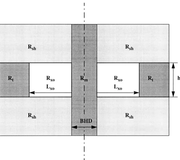
The formation model geometry used throughout this thesis is shown in Figure 2-1. The major assumptions regarding the model are the following:

* it is symmetric with respect to the borehole axis;

* the model is two-dimensional: the resistivity changes both vertically (from layer to layer) and radially (borehole, invaded zone, undisturbed formation);

* in the vertical direction, the model consists of layers of different thicknesses parallel to the surface and perpendicular to the borehole axis;

* radially, the borehole and invaded zones within layers represent concentric cylinders around the borehole axis, perpendicular to the layer boundaries (i. e the resistivity variation within a layer is determined not by a different formation mineral content but by a variation in fluid saturation).

Figure 2-1 shows parametrization of the subsurface as applied in the inversion. The following notation is used in this figure and throughout this thesis:

borehole: Rm = mud resistivity, ohm-m; BHD = borehole diameter, m;

invaded zone: Rxo = resistivity of invaded zone, ohm-m;

Lxo = depth of invasion (BHD + 2*Lxo = diameter of invasion), m;

uncontaminated zone: Rt = uncontaminated zone, or true, resistivity, ohm-m;

Rsh = shoulder bed resistivity, ohm-m.

The figure shows the simplest two-dimensional earth model consisting of three layers, two of them being "shoulders" described by a single resistivity, and the middle layer being the "target" layer. The layer of interest is described by the resistivities of the invaded and uncontaminated zones and the diameter of invasion.

I

borehole:

invaded zone:

uncontaminated zone:

Rm = mud resistivity;

BHD = borehole diameter, m; Rxo = resistivity of invaded zone;

Lxo = depth of invasion, m;

Rt = uncontaminated zone, or true, resistivity;

2.2

Borehole resistivity sounding

Electric resistivity of the rocks depends on many factors, such as rock mineral content, porosity, temperature and pressure conditions, formation water mineralization, and the content of the fluid saturating the rock. Hence, it can help us determine the section lithology, structure of the rocks, hydrocarbon content, estimated formation net pay, etc.

The apparent resistivity of the rocks around the borehole is usually determined by the mea-surements of potential difference AU or electric field E caused by the current source of magnitude I. In an isotropic medium, the differential form of Ohm's Law takes the form:

j = GE , _(2.1)

where j is current density, 0 is the conductivity of the medium, and E is the gradient of a scalar

potential:

E = -gradU. _(2.2)

The relationship between the electric resistivity (conductivity) of the isotropic medium, cur-rent density, electric field, and potential can then be written as:

1 au

j = aE = p .. (2.3)

p ar

where r is the distance between the current source and the point of measurement. In an isotropic medium, the magnitude of p in the formula above is the true resistivity of the medium, while in a nonisotropic medium it is its apparent resistivity

pa-Let us consider a point current source of magnitude I at a point A in a homogeneous isotropic medium of resistivity p. For a sphere of arbitrary radius r with the center at the current source, the current is evenly distributed on the surface of a sphere and its density is

I I

J S = 4. r2 (2.4)

Figure 2-2 shows the current lines and equipotential surfaces for a homogeneous formation of infinite thickness. From equation (2.3) if follows that

ju

E = r j p . _(2.5)

Substituting (2.4) in (2.5), integrating and neglecting the integration constant (I=0 when r

approaches infinity), we obtain:

U 4r _(2.6)

Let the electric field potentials be measured at the electrodes M and N at the respective dis-tances from the source rl = AM and r2 = AN. If the current return electrode is considered to be

infinitely far from the point of measurement, then the potential difference is

pA- I 1 1 p.I MN

AU - A-M IN = _AM.AN

(2.7)

The resistivity or, in a nonhomogeneous case, the apparent resistivity is then

K-AU Pa = (2.8) where AM -AN K = 4xt. MN

is the sonde geometric factor usually referred to as the K-factor.

Lateral sounding

Normal and lateral sondes were the first devices invented for measuring formation resistivity. They appeared both in Russia and the U.S. in the late 1920's -early 1930's. (C. Schlumberger con-ducted the first electrical logging runs in 1926 - 1928.) Both sondes consist of four electrodes, one on the surface and three downhole with different arrangements. One pair of electrodes emits and receives the survey current and the other pair measures the potential drop in the formation.

-10

-4

_S-2

Radial Distance (feet)

Figure 2-2. Computed current patterns (arrows) and equipotential surfaces for a normal sonde in a homogeneous formation. (After Gianzero, S., Anderson, B., Introduction, 1992)

The current electrode on the surface is often considered to be at infinite distance from the point of measurement, and one usually speaks of a three-electrode nonfocused measurement scheme. With a scaling change, the potential difference is then presented as a log of apparent resistivity (see formula (2.8)).

Figure 2-3 shows the electrode arrangements for both normal and lateral sondes. The current and measuring electrodes are usually denoted as pairs: (A and B) and (M and N), respectively. For a normal sonde, the distance between the two "nonpaired" electrodes is considerably smaller than the distance between the "paired" ones (AM<<MN or AM<<AB), and vice versa for a lateral sonde (MN<<AM or AB<<AM).

Utilization of the lateral sounding technique for analysis of radial resistivity distribution repre-sents the key difference of Russian resistivity logging compared to the West. The essence of the method consists in measuring apparent resistivity opposite to the interval being studied by means of lateral and normal sondes of various spacings. It allows us to discover the existence of strata penetrated by the drilling mud, as well as the resistivities of the invaded zone and the undisturbed part of the formation and the depth of penetration with sufficient accuracy.

In general, both normal and lateral sondes also include those with two current and one mea-suring electrodes in the borehole. However, they are rarely used and are not shown in Figure 2-3. The main reason for placing the current return electrode on the surface is to avoid the Delaware effect. If the current return electrode B is downhole, in the presence of very resistive formations, the path of the least resistance to the return is through the borehole. Since B is a current sink, it drives the potential of the reference electrode N below the value it would have had in the absence of the resistive formation. The result is a gradual and substantial increase in measured resistivity as B and N enter the resistive medium, even though the sonde itself is far removed from the resis-tive medium.

The size (or length) of the normal sonde is the distance between the nonpaired electrodes Lnorm = AM. The recording point is referred to as O and is considered to be at half-distance between A and M (Figure 2-3a). For a lateral sonde, the size L is the distance from the nonpaired distant electrode to half distance between the paired electrodes, the latter being also the measure-ment point Llat = AO (Figure 2-3b). Figure 2-3c shows a lateral sonde in the borehole.

Meter Generator

B 711

-current electrodes (A, B)

/A \

A

m]

M

(c) N

Figure 2-3. Electrode arrangements for (a) normal sondes; (b) lateral sondes; (c) borehole example (lateral sonde).

The suite of the so called "standard logging" curves that are run in most boreholes includes five direct (bottom) lateral sondes of the following sizes: L = 0.45, 1.05, 2.25, 4.25, and 8.50 m; one inverted (top) lateral sonde L = 2.25 m; and one normal sonde L = 0.5 m. Some sondes or their sizes may vary depending on a specific borehole environment or on a particular problem. The normal sonde has a symmetric response and provides the apparent resistivity measurements which are very close to the true resistivity in resistive layers of great thickness. However, they prove highly unreliable in thin layers, as we will show later. The lateral sondes, having various depths of investigation, provide the information about the resistivity variation away from the bore-hole. The top lateral sonde is often used in manual interpretation for adjusting the layer bound-aries (if the log is well differentiated) as well as in quantitative interpretation.

Theoretical responses: lateral sondes

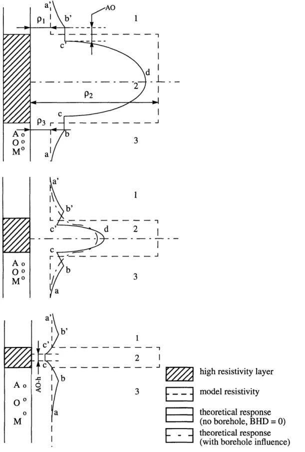
Figure 2-4 shows an example of the theoretical response of an "ideal" lateral sonde (the dis-tance between the measuring electrodes MN -> 0) against resistive layers of different thicknesses surrounded by conductive shoulders. The solid lines represent the responses without borehole influence. Figure 2-4b also shows an example of borehole influence on the response in a dashed line.

For a layer of large thickness (thickness considerably larger than the tool size, h > AO), the response consists of five intervals corresponding to the process of moving the tool along the bore-hole (Figure 2-4a). Intervals ab, de and gh correspond to the period of time when all electrodes are in the same layer (lower shoulder 3, resistive layer 2, or upper shoulder 1, respectively). For intervals bc and ef, the tool is positioned in such a way that the current and potential electrodes are in different layers and hence are divided by a layer boundary.

Figure 2-4 shows that the responses of lateral sounding tools are asymmetric with respect to the center of layer 2 even if pi and p3 are equal. Note that in layer 2 the apparent resistivity above the middle of the layer is lower than the true resistivity P2, while below the middle of the layer the apparent resistivity is greater than P2. It is caused by the change in current density when crossing the layer boundaries. The current tends to flow downward below the middle of layer 2 (since P2 >

1

2

high resistivity layer model resistivity

-- I _ -t theoretical response

00 I b (no borehole, BHD = 0)

_ . theoretical response

a _{(with borehole influence)}

Figure 2-4. Theoretical responses of the bottom lateral sondes against resistive layers of dif-ferent thicknesses surrounded by conductive layers (pl < P2 > p3).

Ao

Oo

Ao

The ratio of apparent to true resistivity measured between the electrodes M and N is deter-mined by the ratio of potential gradients between M and N in nonhomogeneous and homogeneous media: Pa _ E _ JPMN j Eand (2.9) PMN EH JHPMN jH Pa = -PMN , (2.10) JH

where jH is the current density in a homogeneous formation.

Hence, for a bottom lateral sonde until the current electrode A crosses the middle of the resis-tive layer, in the lower part j is greater than jH and Pa > P2, and in the upper part j is lower than jH and Pa < P2. Based on this fact, the layer boundaries for an ideal lateral sonde are picked at the maximum (bottom) and minimum (top) apparent resistivity points.

Interval ef (ef= AO) corresponds to the tool positions when potential electrodes MN are cross-ing the upper boundary and until the electrode A enters the resistive layer. The ratio of the current reflected by the upper boundary into layer 1 to the current transmitted into layer 2 is then deter-mined by the ratio p2/P 1. _{When j << jH, Pa = (J/jH)P2, and Pa <<}

P2-When the thickness of the layer is approximately equal to the tool size (h - AO), the resistivity

efincreases (Figure 2-4b). This results from the influence of not only the upper but also the lower

shoulder, where the current density is higher.

For a very thin layer and large AO (h < AO), the maximum apparent resistivity of layer 2 decreases dramatically (Figure 2-4c). This results from the strong influence of the shoulders. One can also see a distinct second local maximum (point b) at the distance AO below the layer 2. The decrease in Pa in the lower halfspace from b to e occurs in the interval equal in length to the thick-ness of layer 2, with the current electrode A moving from the bottom to the top of layer 2. From e to c, the current electrode is already above layer 2 and j << jH, Pa = (iljH)P3 and Pa <<

P3-The theoretical responses for the top lateral sondes (when the current electrode is placed below the measuring ones) can be explained in the same way and will represent approximately the mirror images of the bottom sondes' theoretical responses.

The above discussion is valid for an "ideal" sonde (MN -> 0). In theory, we would like MN to approach zero to obtain the most accurate potential difference log. However, in a real case the sig-nal level of the tool does not allow us to register the difference in potential change over very small distances. For the largest commonly used lateral sonde (AO = 8.5 m), the distance MN is equal to

1 m. Figure 2-5 corresponds to the theoretical response in such a case. The local anomaly in the lower halfspace stays unchanged since it is caused by the moving of the same current electrode A across the boundaries. The response is different from an "ideal" case only in the intervals where the boundaries are being crossed by the measuring electrodes. The magnitude of pMN and hence, Pa, changes more gradually, effectively smoothing out the curve. The extremum points corre-sponding to the layer boundaries move up by the distance MN/2. (For a top sonde they will move down by the distance MN/2.)

Theoretical responses: normal sondes

Figure 2-6 shows the theoretical responses of the normal sondes of different sizes for a high resis-tivity layer surrounded by conductive shoulders. "Ideal" normal sonde responses are always sym-metric with respect to the center of the layer, because a bottom sonde AM is absolutely equivalent to a top sonde MA. Hence, in our discussion of normal theoretical responses, we can omit either

half of the layer.

For a layer of a large thickness (h > AO), the response in the lower half of the layer consists of three intervals (Figure 2-6a). Intervals ab and cd correspond to the sonde positions where all elec-trodes are in the same layer (lower shoulder 3 or resistive layer 2). For the interval bc, the current and potential electrodes are divided by a layer boundary.

The formulas (2.9) and (2.10) for a normal sonde become:

Pa _ UM

SU , and (2.11)

PM UH

UM

2

MN/2

m high resistivity layer

Mo __ model resistivity 00 No _ theoretical response (ideal sonde) a theoretical response (MN > 0)

I 1 d 2 b 3 1 2 I -4

high resistivity layer

3 _ model resistivity

I theoretical response (no borehole, BHD = 0)

[_T theoretical response (with borehole influence)

Figure 2-6. Theoretical responses of normal sondes against resistive layers of different thick-nesses surrounded by conductive layers (pl < P2 > _P3).

Ao O o MO 00 a' b' c S b a

where UH is the potential in a homogeneous formation. In the interval ab, the apparent resistivity increases with the sonde approaching the bottom of the resistive layer as the potential in the lower halfspace increases. For a thick layer, the resistivity in the interval bc hardly changes (Figure 2-6a); however, with the size of the tool approaching the layer thickness, it decreases slightly (Fig-ure 2-6b). This is caused by the current leaking into the upper halfspace and thus decreasing the potential at the measuring electrode M. The smaller the layer thickness, the sharper the potential drop.

In the interval cd, the apparent resistivity increases sharply and in thick layers approximately reaches the true resistivity in layer 2. For AM approaching the layer thickness (AM - h), the readings at the middle point are considerably lower than the true resistivity because of the current leakage into the upper halfspace (Figure 2-6b). Again, the thinner the layer, the greater the influence of the shoulder layers on the readings in resistive layer 2.

When AM < h (Figure 2-6c), the normal sonde response is distorted due to the fact that the current does not tend to flow into the resistive layer. Only the ab interval stays similar to that in the above figures. After the current electrode A crosses the upper boundary of layer 2, the two electrodes are divided by a thin resistive layer. This results in the minimum readings against the resistive layer until electrode M reaches the bottom of it, producing the interval cc' whose length is equal to (AM -h).

Due to such a high uncertainty in the readings of normal sondes in thin resistive layers, we did not use normal measurements in the inversion process. However, normal logs can be taken into account by comparing them with the theoretical responses calculated for the earth models resulting from inversion. The quality of normal logs can also be estimated from such a comparison.

Effect offormation parameters on lateral theoretical responses

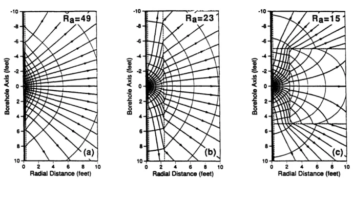
Let us now consider the responses affected by the changes in resistivity and depth of invasion from layer to layer. Figures 2-7a-c show the current patterns calculated for the earth models described with different numbers of parameters. Figure 2-7a shows the current and equipotential lines for the case of a homogeneous halfspace influenced only by borehole drilling mud; Figure 2-7b is also influenced by the invaded zone resistivity; Figure 2-7c illustrates a realistic case also affected by the layer thickness.

2 4 6 8 10 0 2 4 6 8

Radial Distance (feet) Radial Distance (feet) Radial Distance (feet)

Figure 2-7. Computed current patterns and equipotential surfaces for a normal sonde showing: (a) borehole effect;

(b) invasion;

(c) a thin bed with invasion

Rxo = 10 ohm-m, Rt = 50 ohm-m, Rsh = 5 ohm-m (After Gianzero, S., Anderson, B., Introduction, 1992)

Figures 2-8 through 2-12 show the theoretical responses of the five lateral measurements described above for the same resistivity earth model, but for different layer thicknesses and invaded zone diameters. The earth model parameters are the following: Rsh = 3 ohm-m, Rxo = 5 ohm-m, Rt = 100 ohm-m, Lxo = 0.5 m (a resistive invaded layer surrounded by conductive

shoul-ders). The borehole diameter is 0.2 m with the mud resistivity Rm = 1 ohm-m. From Figure 2-8 to 2-10 the thickness of the layer decreases from 10 m to 2 m to 0.5 m. The shaded area shows the invasion profile. For the thick layer (Figure 2-8), it is evident that the deeper the measurement, the less it is affected by the invaded zone, and consequently the closer its readings are to the true for-mation resistivity.

In Figures 2-9 and 2-10, one can clearly see the local maxima below the resistive layer in cases when the sonde size is larger than the layer thickness. For a 2-meter layer, only the two deepest measurements have these second maxima, while for a 0.5-meter layer all measurements except for the shallowest one (LO.45) are considerably affected by the layer thickness. For the 10-meter layer, any visible influence of the bed thickness is reflected below the resistive layer only on the deepest measurement (L8.50), since its depth of investigation is of the order of the layer

thick-ness.

Figure 2-11 illustrates the theoretical responses for a multi layer model. The resistivities in the high resistive layers are the same as above, while in conductive layers Rt (or Rsh) = 3 ohm-m.

Note that in the resistive layers the shallow measurements (for LO.45 and L1.05, AO < h) are roughly the same, while the deeper measurements differ, resulting from the effect of the current electrode crossing the boundaries as described above. In the deepest response, one can also see the superposition of the second maxima resulting from the two resistive layers.

Figure 2-12 shows the influence of the depth of invasion on the tool responses for a 2-meter layer (resistivities are the same as above). The depth of invasion changes from 0.2 to 0.5 to 1 m (the shaded area is the invasion profile), and obviously the larger the depth of invasion, the harder it is for the tool to "reach" the true formation resistivity. This results in the curves being less dif-ferentiated since the resistivities of the shoulders and the invaded zone are considerably lower than that of the uncontaminated formation.

Figure 2-8. Lateral sounding theoretical responses for a 10-meter layer.

Model: Rsh= 3, Rxo = 5, Rt = 100 ohm-m, Lxo = 0.5 m.

I-0.2 Model Rt Model Lxo R mrn) ohm-m)

L

I

H

I

I I I I

Figure 2-9. Lateral sounding theoretical responses for a 2-meter layer.

Model: Rsh = 3, Rxo = 5, Rt= 100 ohm-m, Lxo = 0.5 m.

0.2 Model Rt 200 0.2 Model Rxo 200 0.2 L 0.45 200 0.2 L 1.05 200 0.2 L 2.25 200 0.2 L 4.25 200 0.2 L 8.50 200 (ohm-m) del R i - Ny' f P

i

iF

-Figure 2-10.Lateral sounding theoretical responses for a 0.5-meter layer.

Model: Rsh = 3, Rxo = 5, Rt= 100 ohm-m, Lxo = 0.5 m.

0.2 _{Model Rt} ,O Model Lxo ID R m 1 .25 < m) (ohm-m) I IF, A~m 0 9 Mndiel Rxn 200 .L 0.45 200 ,,.,2, ... L . ... ... 0.2 L 2.25 200 0. L 4.25 200 0.2 L 8.50 200 (ohm-m) P1 1Rxo mo l.Z i Ef

Figure 2-11. Lateral sounding theoretical responses for a multi layer model.

Conductive layers: Rt = 3 ohm-m; resistive layers: Rxo = 5, Rt = 100 ohm-m, Lxo = 0.5 m.

0.2 Model Rt 0. 2 Model Rxo 20 0.2 L 0.45 200 0.2 L 1.05 200 0.2 L 2.25 200 0.2 L 4.25 200 0.2 L 8.50 200 (ohm-m )

Lxo = 0.2 m Lxo = 0.5 m

0.2 Model Rt 200

INVADED ZONE 0.2 Model Rxo 200

0.2 LU.43 200 0.2 L 1.05 200 Model Lxo Rm 0.2 L2.25 200 0 1 0 1.25 L4.25 0.2 4.25 200 (m) (ohm-m) 0.2 L 8.50 Lao ( ohm-m)

11t. ff it

111111111 111111111

2.3 Laterolog

One of the major disadvantages of lateral sounding is its relatively low vertical resolution. It results from the fact that the current from the point source flows in the borehole in all directions, leading to borehole and shoulder effects. The idea of forcing the current to flow into the formation against which the potential difference is being measured has been implemented in the laterolog device (Doll, 1951). The simplest laterolog device (LL3) is comprised of three electrodes: a survey current electrode located in the center of the array surrounded by two elongated guard electrodes, forcing the emitted currents to be perpendicular to the surface of the mandrel as shown in Figure 2-13. The smaller the center electrode, the more highly resolved the measurement.

In LL3, a constant current is applied to the center electrode. An auxiliary current of the same polarity is applied to the guard electrodes. The guard electrode current is automatically and continuously adjusted to maintain a zero potential difference between the center electrode and the guard electrodes. This forces the current emanating from the current electrode to flow into the formation. A drop in potential is caused by the flow of the current through the surrounding formation to a remote current return electrode. This potential difference is related to the resistivity of the formation.

The accuracy of the measurement is greatly enhanced by designing the array to focus on the zone of interest. With a laterolog, we still need a conductive borehole environment in order to transmit the current from the electrodes to the formation. However, the mud column has much less influence on laterolog readings than with lateral nonfocused methods.

The depth of investigation of LL3 is approximately 1-2 meters. With very shallow depths of invasion, the laterolog provides the apparent resistivity close to the true formation resistivity. One of the disadvantages of the LL3 lies in its limited depth of investigation. Having a single resistivity measurement (or even two measurements, shallow and deep, as in a Dual laterolog, which is not considered in this thesis), it is difficult to determine the resistivity distribution away from the borehole as well as the depth of invasion.

Figure 2-14 shows theoretical LL3 responses for a complicated earth model. We have three invaded layers divided by conductive shoulders. The borehole diameter is 0.2 m with the mud Rm = 1 ohm-m. In a resistive layer with Rxo << Rt the response is determined by the depth of

(VI)

,---_-I

(V0)

(V2)

Figure 2-13. Laterolog (LL3) electrode configuration. 12

IA

Figure 2-14. Laterolog theoretical responses for a sequence of layers. Rsh = 3, Rm = 1 ohm-m, layer 1: Rxo = 5, Rt = 100 ohm-m, Lxo = 0.5 m;

layer 2: Rxo = 5, R_t = 100 ohm-m, Lxo = 0. 1 m; layer 3: Rxo = 100, Rt = 5 ohm-m, Lxo = 0.5 m.

approaching Rt. However, with deeper invasion, Lxo = 0.5 m (layer 1), the influence of invaded

resistivity zone is substantial. In layer 3, the formation is more conductive than the invaded zone which leads to the characteristic "horns" (sharp decreases of resistivity) on the layer boundaries. The latter situation is not favorable for laterologs.

2.4 Summary

In this thesis, we are aiming to combine lateral sounding and laterolog techniques in order to provide both a mathematically accurate and physically meaningful solution. Lateral sounding measurements enable us to thoroughly examine the resistivity distribution away from the borehole and solve for both the invaded zone and the undisturbed zone parameters. However, vertical resolution of sounding measurements, especially the deeper ones, is not very high. Since the current is allowed to flow from the emitting electrode in all directions, the lateral sounding measurements are not very sensitive to layer boundaries with low layer resistivity contrasts. On the other hand, the laterolog uses guard electrodes held at the same potentials as the current electrode, to force the current to flow into the formation. This reduces the influence of shoulder beds and allows us to read the apparent resistivities very close to the true undisturbed formation resistivities in zones with shallow invasion. The laterolog also has a higher vertical resolution of the boundaries than the nonfocused measurements. The combination of both methods provides us with a most comprehensive and detailed picture of the resistivity distribution in both radial and vertical directions.

Chapter 3

Forward modeling and inversion

3.1 General considerations

The mathematical basis for any inversion is finding the best fitting earth model for the field data by means of minimizing the difference between the data and model theoretical responses. With the earth parametrized by layer thicknesses and resistivities, as shown in Figure 2-1, we first choose the initial earth model. The initial guess is a set of particular physical and geological conditions for which synthetic tool responses are generated and compared to the field data. The more information we have about such conditions for the data, the more educated is our initial guess, and hence, the faster we get to the solution. If we are not satisfied with the result, we keep changing the model parameters and simulating the responses until a predefined condition of convergence is met. Convergence criteria allow us to evaluate the misfit between the theoretical and field data. The process of varying the model parameters to achieve an acceptable data approximation is called optimization. Thus, in general, inversion depends on and is limited by * forward modeling algorithms;

* optimization strategy;

* types and quality of the data available.

The principles of the forward modeling and inversion algorithms, as well as the optimization technique employed in the inversion software developed by Western Atlas Logging Services, are described in this chapter. The types and quality of data used in both synthetic and field data examples are discussed in Chapters 4 and 5.

3.2 Forward modeling principles

An effective forward modeling algorithm is always one of the main challenges in any iterative procedure. The technique of fast numerical simulation of induction and resistivity logs has been developed by Tamarchenko and Druskin (1993). A hybrid approach, consisting of a combination of integral equations and finite-difference schemes, is applied to a Green's function problem. An analytical representation of the solution is obtained in each layer in the vertical direction, and the radial distribution of the field is approximated on an expanding grid. The

solution is then matched on the layers boundaries, leading to a tri-diagonal system of linear algebraic equations, where each element is a matrix. What follows is the description of the main principles employed in the numerical simulation algorithm. For detailed information on integral equations and numerical implementation, the reader is referred to Tamarchenko and Druskin (1993).

Figure 3-1 (a) shows the subsurface geometry for numerical simulation. The model is axially symmetric, with horizontal layers, intersected by a vertical cylindrical borehole. Each layer con-tains, or may contain, an invasion zone with cylindrical boundaries coaxial with the borehole.

Let us explain the theoretical principles of the forward modeling code using the example of a simplified three-layer model intersected by the insulating mandrel as shown in Figure 3-1 (b). Note that the borehole and invaded zone are not included.

The electromagnetic field distribution is described by a partial differential equation. For a DC current, the function u(x, s) represents a potential of a circular electrode positioned at a point

s =(rs, zs) and measured at the point x = (r, z). The function u(x, s) satisfies the following

equa-tion:

a

au

a

au

r(r,z) + ra(rz)- = 8(r-rsZ-zs) , (3.1)

where a(r, z) is the conductivity of the medium and 8 (r-rs, z-zs) is the delta function.

Let us consider an i-th layer surrounded by the shoulders of different resistivities. In order to find the analytical solution for potential u at a point (ro, z0), we introduce an auxiliary point source

V in the layer i. The source potential v satisfies the following equation:

a

a

ro(r, (r z) r(r, z) -8(r - r, z - zo) . (3.2)

ar

ar az

az

We can now express the electric potential u(ro, z0) in the layer i using Green's theorem:

(

av

au

u(ro, zo) = -U v dS . _(3.3)

(b) U (current electrode) Pi-1 - Si I(b) I I I I I I I I I I I (contour area) V (auxiliary (c)---- surce) Pi+1 mandrel

Figure 3-1. Forward modeling:

(a) 2-dimensional earth model with the tool positioned in the borehole; (b) simplified layered structure without borehole.

borehole

-1 - --- ^ --- --- --- I I-I~ r - - I~" I-~I - - r

Sis _{the normal derivative at the surface S directed outwards. If we assume a homogeneous}

an

environment for the Green's function everywhere outside the i-th layer (i.e. pi_- = pi = Pi+l), then the equation (3.2) for the auxiliary potential v can be simplified to:

2

2- k Vk

a ₂

= -6(z- z0), k = 1, 2... _, (3.4)

where Xk2 are the eigenvalues of the operator -r a ( monic of the potential v from the following equation:

a OVk 2

ro(r)-r + k ry(r)Vk = 0

The formula (3.3) for an i-th layer becomes:

ui(ro, zo) = ui(ro, zo)+-

ui,

Si

and

r, _{)F , and vk is the corresponding}

har-,k= 1, 2...oo

+ Vi.-

)dS

a~n)

The uio(r0, z0) term in equation (3.6) appears only in the case when the current electrode is located

in the same layer where the potential ui is being determined.

On each horizontal boundary, both the potential and the current normal to the boundary are continuous, which can be expressed for an i-th layer in the following form:

aui aui+ 1

ui = ui+1 ,and O i = (i+ ₁ +

Equating the potentials on each boundary (left-hand side of equation (3.3)), we end up with a sys-tem of integral equations. The potential ui satisfies the Newman boundary condition on the

man-drel surface:

aui an

The selection of the Newman boundary condition for the Green's function v on the surface of the mandrel

(3.5)

avi ₀

-0

an

allows us to reduce the surface of integration, i.e. to eliminate the interval (b) of the surface Si as shown in Figure 3-1 (b).

Thus, applying Green's theorem in each layer and matching the potentials and current fluxes on the plane boundaries, we obtain a blocked tri-diagonal system of integral equations. The verti-cal direction is treated analytiverti-cally, which proves to be computationally effective when dealing with hundreds of meters of data involving large numbers of layers. Radially, the differential oper-ator in equation (3.5) is approximated with a finite-difference scheme on an expanding grid. Depending on the desired accuracy of the solution and the depth of investigation of a particular tool, it is possible to adjust the number of nodes in the grid as well as the distance between them.

Note that this method can be used for any type of radial conductivity distribution. The only requirement is to have enough nodes in the radial grid to approximate the field behavior properly. With such considerations, the borehole and invaded zones can be easily incorporated into our sim-plified formation model.

3.3 Inverse problem

In this thesis, we shall consider only the discrete case of the inversion problem. The detailed description of the continuous case can be found in Mezzatesta (1996). In general, an inversion problem can be stated as:

d = F(x)+e , _(3.7)

where the data vector d = col (dl, d2 ... dn) of N observations is a function of the model

parameters vector x = col (xl, x2 ... xm) of M parameters, and e is the error vector due to the

finite accuracy of the measurements.

Let us denote f = col (fl, f2 ... fn) the model theoretical response vector of size N for a

particular set of parameters. A perturbation of the model response about the initial set of parameters xo can be represented by the first order Taylor expansion:

(3.8)

f(x) = f(x + Ax) = fo + Ax + HOT

j=1 x = Xo

where Axj = xj - xj,o represents the formation parameter change vector. Neglecting higher order terms (H.O.T.), equation (3.8) can also be written as:

Af(xo) = fxo)Ax ,

j= 1

(3.9)

where Af is the absolute change in tool responses to variations in formation parameters. In matrix form, we write:

Af = JAx _(3.10)

In this equation, J is the NxM Jacobian matrix of derivatives evaluated at x0for each data point:

af x, J=af ax,

1f

In many cases it is convenient to have the Jacobian in dimensionless form. For that, we have to consider relative increments 8fiand 8xj, defined as:

,and xj = X

Xj , i = 1,2,...N; j = 1, 2,...M. (3.12)

Defining the diagonal matrices,

fi # 0 , i, j = 1,2,...N, and

f

j

Xi = i, =

0, i

j)

xi _{0 ,i,j = 1,2,...M,}

the following equation holds:

FAf = FG(X- X)Ax = (FGX-)XAx . (3.15)

According to the definition of relative increments, the following relations apply:

8f = FAf and Sx = XAx (3.16)

Then the relationship between the relative increments and the earth model parameters becomes:

5f = (FGX-')Sx = Fx , (3.17)

where F is the matrix J in dimensionless form, containing the bilogarithmic derivatives as entries, i.e.: Xj = fi fi xj _ lnf , i = 1, 2,...N; j = 1, 2,...M. alnxj (3.18)

We can now rewrite equation (3.17) in vector form:

j=X anxlnx (3.19)

Equations (3.17) and (3.19) represent the total relative variation of the response vector f due to individual relative variation of the parameter vector x, in the vicinity of an initial model x0.

Throughout the following discussion, we will keep the more familiar J notation for the Jaco-bian matrix, bearing in mind that it is in fact the dimensionless form of it.

Singular Value Decomposition (SVD)

In order to solve equation (3.10) as well as any inversion problem, we need to invert matrix J. Sin-gular value decomposition (SVD) is one of the most powerful methods for matrix inversion. It (3.14)