BY
ROGER KAUFMANN, ANDREAS GADMER AND RALF KLETT
ABSTRACT
In the last few years we have witnessed growing interest in Dynamic Financial Analysis (DFA) in the nonlife insurance industry. DFA combines many eco-nomic and mathematical concepts and methods. It is almost impossible to identify and describe a unique DFA methodology. There are some DFA soft-ware products for nonlife companies available in the market, each of them relying on its own approach to DFA. Our goal is to give an introduction into this field by presenting a model framework comprising those components many DFA models have in common. By explicit reference to mathematical language we introduce an up-and-running model that can easily be imple-mented and adjusted to individual needs. An application of this model is pre-sented as well.
KEYWORDS AND PHRASES
Nonlife insurance, Dynamic Financial Analysis, Asset/Liability Management, stochastic simulation, business strategy, efficient frontier, solvency testing, inter-est rate models, claims, reinsurance, underwriting cycles, payment patterns.
1. WHAT is DFA
1.1. Background
In the last few years, nonlife insurance corporations in the US, Canada and also in Europe have experienced, among other things, pricing cycles accompa-nied by volatile insurance profits and increasing catastrophe losses contrasted by well performing capital markets, which gave rise to higher realized capital gains. These developments impacted shareholder value as well as the solvency position of many nonlife companies. One of the key strategic objectives of a
1
The article is partially based on a diploma thesis written in cooperation with Zurich Financial Ser-vices. Further research of the first author was supported by Credit Suisse Group, Swiss Re and UBS AG through RiskLab, Switzerland.
214 R. KAUFMANN, A. GADMER AND R. KLETT
joint stock company is to satisfy its owners by increasing shareholder value over time. In order to achieve this goal it is necessary to get an understanding of the economic factors driving shareholder value and the cost of capital. This does not only include identifying the factors but investigating their random nature and interrelations to be able to quantify earnings volatility. Once this has been done various business strategies can be tested in respect of meeting company objectives.
There are two primary techniques in use today to analyze financial effects of different entrepreneurial strategies for nonlife insurance companies over a specific time horizon. The first one - scenario testing - projects business results under selected deterministic scenarios into the future. Results based on such a scenario are valid only for this specific scenario. Therefore, results obtained by scenario testing are useful only insofar as the scenario was cor-rect. Risks associated with a specific scenario can only roughly be quantified. A technique overcoming this flaw is stochastic simulation, which is known as
Dynamic Financial Analysis (DFA) when applied to financial cash flow
mod-elling of a (nonlife) insurance company. Thousands of different scenarios are generated stochastically allowing for the full probability distribution of important output variables, like surplus, written premiums or loss ratios.
1.2. Fixing the Time Period
The first step to compare different strategies is to fix a time horizon they should apply to. On the one hand we would like to model over as long a time period as possible in order to see the long-term effects of a chosen strategy. In particular, effects concerning long-tail business only appear after some years and can hardly be recognized in the first few years. On the other hand, simu-lated values become more unreliable the longer the projection period, due to accumulation of process and parameter risk over time. A projection period of five to ten years seems to be a reasonable choice. Usually the time period is split into yearly, quarterly or monthly sub periods.
1.3. Comparison to ALM in Life Insurance
A DFA model is a stochastic model of the main financial factors of an insur-ance company. A good model should simulate stochastically the asset ele-ments, the liability elements and also the relationships between both types of random factors. Many traditional ALM-approaches (ALM = Asset/Liability Management) in life insurance considered the liabilities as more or less deter-ministic due to their low variability (see for example Wise [43] or Klett [25]). This approach would be dangerous in nonlife where we are faced with much more volatile liability cash flows. Nonlife companies are highly sensitive to inflation, macroeconomic conditions, underwriting movements and court rulings, which complicate the modelling process while simultaneously making results less certain than for life insurance companies. In nonlife both the date
of occurrence and the size of claims are uncertain. Claim costs in nonlife are inflation sensitive, whereas they are expressed in nominal terms for many tra-ditional life insurance products. In order to cope with the stochastic nature of nonlife liabilities and assets, their number and their complex interactions, we have to rely on stochastic simulations.
1.4. Objectives of DFA
DFA is not an academic discipline per se. It borrows many well-known con-cepts and methods from economics and statistics. It is part of the financial management of the firm. As such it is committed to management of prof-itability and financial stability (risk control function of DFA). While the first task aims at maximizing shareholder value, the second one serves main-taining customer value. Within these two seemingly conflicting coordinates DFA tries to
• strategic asset allocation, • capital allocation, • performance measurement, • market strategies, • business mix, • pricing decisions, • product design, • and others.
This listing suggests that DFA goes beyond designing an asset allocation strategy. In fact, portfolio managers will be affected by DFA decisions as well as underwriters. Concrete implementation and application of a DFA model depends on two fundamental and closely related questions to be answered beforehand:
1. Who is the primary beneficiary of a DFA analysis (shareholder, management, policyholders)?
2. What are the company individual objectives?
The answer to the first question determines specific accounting rules to be taken into account as well as scope and detail of the model. For example, those companies only interested in getting a tool for enhancing their asset allocation on very high aggregation level will not necessarily target a model that emphasizes every detail of simulating liability cash flows. Smith [39] has pointed out that making money for shareholders has not been the primary motivation behind developments in ALM (or DFA). Furthermore, relying on the Modigliani-Miller theorem (see Modigliani and Miller [34]) he put for-ward the hypothesis that a cost benefit analysis of asset/liability studies might reveal that costs fall on shareholders but benefits on management or customers. Our general conclusion is that company individual objectives - in particular with respect to the target group - have to be identified and formulated before starting the DFA analysis.
216 R. KAUFMANN, A. GADMER AND R. KLETT
1.5. Analyzing DFA Results Through Efficient Frontiers
Before using a DFA model, management has to choose a financial or eco-nomic measure in order to assess particular strategies. The most common framework is the efficient frontier concept widely used in modern portfolio theory going back to Markowitz [32]. First, a company has to choose a return measure (e.g. expected surplus) and a risk measure (e.g. expected policyholder deficit, see Lowe and Stanard [30], or worst conditional mean as a coherent risk measure, see Artzner, Delbaen, Eber and Heath [2] and [3]). Then the mea-sured risk and return of each strategy can be plotted as shown in Figure 1.1. Each strategy represents one spot in the risk-return diagram. A strategy is called efficient if there is no other one with lower risk at the same level of return, or higher return at the same level of risk.
return
risk FIGURE 1.1: Efficient frontier.
For each level of risk there is a maximal return that cannot be exceeded, giving rise to an efficient frontier. But the exact position of the efficient frontier is unknown. There is no absolute certainty whether a strategy is really efficient or not. DFA is not necessarily a method to come up with an optimal strategy. DFA is predominantly a tool to compare different strategies in terms of risk and return. Unfortunately, comparison of strategies may lead to completely different results as we change the return or risk measure. A different measure may lead to a different preferred strategy. This will be illustrated in Section 4. Though efficient frontiers are a good means of communicating the results of DFA because they are well-known, some words of criticism are in place. Cumberworth, Hitchcox, McConnell and Smith [10] have pointed out that there are pitfalls related to efficient frontiers one has to be aware of. They criti-cize that typical efficient frontier uses risk measures that mix together system-atic risk (non-diversifiable by shareholders) and non-systemsystem-atic risk, which blurs the shareholder value perspective. In addition to that, efficient frontiers might give misleading advice if they are used to address investment decisions once the concept of systematic risk has been factored into the equation.
1.6. Solvency Testing
A concept closely related to DFA is solvency testing where the financial posi-tion of the company is evaluated from the perspective of the customers. The central idea is to quantify in probabilistic terms whether the company will be able to meet its commitments in the future. This translates into determin-ing the necessary amount of capital given the level of risk the company is exposed to. For example, does the company have enough capital to keep the probability of loosing a • 100% of its capital below a certain level for the risks taken? DFA provides a whole probability distribution of surplus. For each level a the probability of loosing a • 100% can be derived from this distribu-tion. Thus DFA serves as a solvency testing tool as well. More information about solvency testing can be found in Schnieper [37] and [38].
stochastic scenario
output
generator
input - historical data - model parameters - strategic assumptions • / / analyze output, revise strategy
FIGURE 1.2: Main structure of a DFA model.
1.7. Structure of a DFA Model
Most DFA models consist of three major parts, as shown in Figure 1.2. The
stochastic scenario generator produces realizations of random variables
repre-senting the most important drivers of business results. A realization of a ran-dom variable in the course of simulation corresponds to fixing a scenario. The second data source consists of company specific input (e.g. mean severity of losses per line of business and per accident year), assumptions regarding model parameters (e.g. long-term mean rate in a mean reverting interest rate model), and strategic assumptions (e.g. investment strategy). The last part, the output provided by the DFA model, can then be analyzed by management in order to improve the strategy, i.e. make new strategic assumptions. This can be repeated until management is convinced by the superiority of a certain strategy. As pointed out in Cumberworth, Hitchcox, McConnell and Smith [10] interpretation of the output is an often neglected and non-appreciated part in DFA modelling. For example, an efficient frontier leaves us still with a
2 1 8 R. KAUFMANN, A. GADMER AND R. KLETT
variety of equally desirable strategies. At the end of the day management has to decide for only one of them and selection of a strategy based on preference or utility functions does not seem to provide a practical solution in every case.
2. STOCHASTICALLY MODELLED VARIABLES
A very important step in the process of building an appropriate model is to iden-tify the key random variables affecting asset and liability cash flows. Afterwards it has to be decided whether and how to model each or only some of these fac-tors and the relationships between them. This decision is influenced by consider-ations of a trade-off between improvement of accuracy versus increase in complexity which is often felt being equivalent to a reduction of transparency. The risks affecting the financial position of a nonlife insurer can be cate-gorized in various ways. For example, pure asset, pure liability and asset/lia-bility risks. We believe that a DFA model should at least address the following risks:
• pricing or underwriting risk (risk of inadequate premiums), • reserving risk (risk of insufficient reserves),
• investment risk (volatile investment returns and capital gains), • catastrophes.
We could have also mentioned credit risk related to reinsurer default, currency risk and some more. For a recent, detailed DFA discussion of the possible impact of exchange rates on reinsurance contracts see Blum, Dacorogna, Embrechts, Neghaiwi and Niggli [5]. A critical part of a DFA model are the interdependencies between different risk categories, in particular between risks associated with the asset side and those belonging to liabilities. The risk of company losses triggered by changes in interest rates is called interest
rate risk. We will come back to the question of modelling dependencies in
Section 5.1. Our choice of company relevant random variables is based on the categorization of risks shown before.
A key module of a DFA model is an interest rate generator. Many models assume that interest rates will drive the whole model as displayed for example in Figure 4.1. An interest rate generator - or economic scenario generator as it is often called to emphasize the far reaching economic impact of interest rates -is necessary in order to be able to tackle the problem of evaluating interest rate risk. Moreover, nonlife insurance companies are strongly exposed to interest rate behaviour due to generally large investments in fixed income assets. In our model implementation we assumed that interest rates were strongly correlated with inflation, which itself influenced future changes in claim size and claim frequency. On the other hand, both of these factors affected (future) premium rates. Furthermore, we assumed correlation between inter-est rates and stock returns, which are generally an important component of investment returns.
On the liability side, we explicitly considered four sources of randomness:
patterns. We simulated catastrophes separately due to quite different statistical
behaviour of catastrophe and non-catastrophe losses. In general the volume of empirical data for non-catastrophe losses is much bigger than for catastrophe losses. Separating the two led to more homogeneous data for non-catastrophe losses, which made fitting the data by well-known (right skewed) distributions easier. Also, our model implementation allowed for evaluating reinsurance programs. Testing different deductibles or limits is only possible if the model is able to generate sufficiently large individual losses. In addition, we currently experience a rapid development of a theory of distributions for extremal events (see Embrechts, Kliippelberg and Mikosch [16], and McNeil [33]). Therefore, we considered the separate modelling of catastrophe and non-cat-astrophe losses as most appropriate. For each of these two groups the number and the severity of claims were modelled separately. Another approach would have been to integrate the two kinds of losses by using heavy-tailed claim size distributions.
Underwriting cycles are an important characteristic of nonlife companies. They reflect market and macroeconomic conditions and they are one of the most important factors affecting business results. Therefore, it is useful to have them included in a DFA model set-up.
Losses are not only characterized by their (ultimate) size but also by their piecewise payment over time. This property increases the uncertainties of the claims process by introducing the time value of money and future inflation considerations. As a consequence, it is necessary not only to model claim fre-quency and severity but the uncertainties involved in the settlement process as well. In order to allow for reserving risk we used stochastic payment patterns as a means of estimating loss reserves on a gross and on a net basis.
In the abstract we pointed out that our intention was to present a DFA model framework. In concrete terms, this means that we present a model implementation that we found useful to achieve part of the goals outlined in Section 1.4. We do not claim that the components introduced in the remain-ing part of the paper represent a high class standard of DFA modellremain-ing. For each of the DFA components considered there are numerous alternatives, which might turn out to be more appropriate in particular situations. Provid-ing a model framework means to present our model as a kind of suggested reference point that can be adjusted or improved individually.
2.1. Interest Rates
Following Daykin, Pentikainen and Pesonen [15, p. 231] we assume strong correlation between general inflation and interest rates. Our primary stochastic driver is the (instantaneous) short-term interest rate. This variable determines bond return across all maturities as well as general inflation and superimposed inflation by line of business.
An alternative to the modelling of interest and inflation rates as outlined in this section and probably well-known to actuaries is the Wilkie model, see Wilkie [42], or Daykin, Pentikainen and Pesonen [15, pp. 242-250].
2 2 0 R. KAUFMANN, A. GADMER AND R. KLETT
2.1.1. Short-Term Interest Rate
There are many different interest rate models used by financial economists. Even the literature offering surveys of interest rate models has grown con-siderably. The following references represent an arbitrary selection: Ahlgrim, D'Arcy and Gorvett [1], Musiela and Rutkowski [35, pp. 281-302] and Bjork [4]. The final choice of a specific interest rate model is not straightforward, given the variety of existing models. It might be helpful to post some general features of interest rate movements, which we took from Ahlgrim, D'Arcy and Gorvett [1]:
1. Volatility of yields at different maturities varies. 2. Interest rates are mean-reverting.
3. Rates at different maturities are positively correlated. 4. Interest rates should not be allowed to become negative.
5. The volatility of interest rates should be proportional to the level of the rate.
In addition to these characteristics there are some practical issues raised by Rogers [36]. According to Rogers an interest rate model should be
• flexible enough to cover most situations arising in practice, • simple enough that one can compute answers in reasonable time, • well-specified, in that required inputs can be observed or estimated, • realistic, in that the model will not do silly things.
It is well-known that an interest rate model meeting all the criteria mentioned does not exist. We decided to rely on the one-factor Cox-Ingersoll-Ross (CIR) model. CIR belongs to the class of equilibrium based models where the instantaneous rate is modelled as a special case of an Ornstein-Uhlenbeck process:
(2.1) dr=K(9-r)dt+arydZ,
By setting y = 0.5 we arrive at CIR also known as the square root process
(2.2) dr,= a(b-rt)dt+s/r,dZt,
where
rt = instantaneous short-term interest rate, b = long-term mean,
a = constant that determines the speed of reversion of the interest rate
toward its long-run mean b,
s = volatility of the interest rate process, (Zt) = standard Brownian motion.
CIR is a mean-reverting process where the short rate stays almost surely pos-itive. Moreover, CIR allows for an affine model of the term structure making the model analytically more tractable. Nevertheless, some studies have shown (see Rogers [36]) that one-factor models in general do not satisfactorily fit
empirical data and restrict term structure dynamics. Multifactor models like Brennan and Schwartz [6] or Longstaff and Schwartz [29] or whole yield approaches like Heath-Jarrow-Morton [20] have proven to be more appropri-ate in this respect. But this comes at the price of" being much more involved from a theoretical and a practical implementation point of view. Our decision for CIR was motivated by practical considerations. It is an easy to imple-ment model that gave us reasonable results when applied to US market data. Moreover, it is a standard model and in widespread use, in particular in the US. Actually, we are interested in simulating the short rate dynamics over the projection period. Hence, we discretized the mean reverting model (2.2) lead-ing to
(2.3) rt=rt
where
rt = the instantaneous short-term interest rate at the beginning of year t,
Z
t~Jf (0,1), Z
uZ
2, ... i.i.d.,
a, b, s as in (2.2).
Cox, Ingersoll and Ross [9] have shown that rates modelled by (2.2) are posi-tive almost surely. Although it is hard for the short rate process to go negaposi-tive in the discrete version of the last equation the probability is not zero. To be sure we changed equation (2.3) to
(2.4) rt = r,_i + a (b - r,-i) + s Jrt-\+ Zt.
A generalization of CIR is given by the following equation, where setting g = 0.5 yields again CIR:
This general version provides more flexibility in determining the degree of dependence between conditional volatility of interest rate changes and the level of interest rates.
The question of what an appropriate level for g might be leads to the field of model calibration which we will encounter at several places within DFA modelling. In fact, the problem plays a dominant role in DFA tempting many practitioners to state that DFA is all about calibration. Calibrating an inter-est rate model of the short rate refers to determining parameters - a, b, s and g in equation (2.5) - so as to ensure that modelled spot rates (based on the instantaneous rate) correspond to empirical term structures derived from traded financial instruments. Bjork [4] calls the procedure to achieve this
inversion of the yield curve. However, the parameters can not be uniquely
determined from an empirical term structure and term structure of volatilities resulting in a non-perfect fit. This is a general feature of equilibrium interest rate models. Whereas this is a critical point for valuing interest rate derivatives, the impact on long-term DFA results may be limited.
222 R. KAUFMANN, A. GADMER AND R. KLETT
With regard to calibrating the inflation model it should be mentioned that building models of inflation based on historical data may be a feasible approach. But it is unclear whether the future evolution of inflation will fol-low historical patterns: DFA output will probably reflect the assumptions with regard to inflation dynamics. Consequently, some attention needs to be paid to these assumptions. Neglecting this is a common pitfall of DFA mod-elling. In order to allow for stress testing of parameter assumptions, the model should not only rely on historical data but on economic reasoning and actuarial judgment of future development as well.
2.1.2. Term Structure
Based on equation (2.2) we calculated the prices F(t, T, (r,)) being in place at time t of zero-coupon bonds paying 1 monetary unit at time of maturity
t + T, as (2.6) where rt\~ 2Ge(a+G)TI2 (a + G)(eGT-l)+2G'
G=Ja
2+2?.
A proof of this result can be found in Lamberton and Lapeyre [27, pp.
129-133]. Note, that the expectation operator is taken with respect to the martin-gale measure <Q assuming that equation (2.2) is set up under the martinmartin-gale measure Q.as well. The continuously compounded spot rates RtT at time t derived from equation (2.6) determine the modelled term structure of zero-coupon yields at time t:
n-n R - lo&F(t,T,(rt))_rtBT-\ogAT
where T is the time to maturity.
2.1.3. General Inflation
Modelling loss payments requires having regard to inflation. Following our introductory remark to Section 2.1 we simulated general inflation /, by using the (annualized) short-term interest rate rt. We did this by using a linear regression model on the short-term interest rate:
where
£,7~^(0,l), e(,e'2,... i l d . ,
a1, b1, a1: parameters that can be estimated by regression, based on historical
data.
The index / stands for general inflation.
2.1.4. Change by Line of Business
Lines of business are affected differently by general inflation. For example, car repair costs develop differently over time than business interruption costs. Claims costs for specific lines of business are strongly affected by legislative and court decisions, e.g. product liability. This gives rise to so-called
super-imposed inflation, adding to general inflation. More on this can be found in
Daykin, Pentikainen and Pesonen [15, p. 215] and Walling, Hettinger, Emma and Ackerman [41],
To model the change in loss frequency df (i.e. the ratio of number of losses divided by number of written exposure units), the change in loss sever-ity df, and the combination of both of them, dt, we used the following for-mulas:
(2.9) Sf=max(aF+bfit+GFsf,-l),
(2.10) df f
(2.H) df=(l
+df)(l
+df)~l,
where
ef~M(0,\), fif, ef, ... i.i.d.,
sf~ JV(0,1), sf, sx, ... i.i.d., EF, EX independent Vtut2,
aF, bF, aF, ax, bx, ax: parameters that can be estimated by regression, based
on historical data.
The variable df represents changes in loss trends triggered by changes in inflation rates, df is applied to premium rates as will be explained in Sec-tion 3, see (3.2). Its construcSec-tion through (2.11) ensures correlaSec-tion of aggregate loss amounts and premium levels that can be traced back to inflation dynamics.
The technical restriction of setting St and df to at least -1 was necessary to avoid negative values for numbers of losses and loss severities.
We modelled changes in loss frequency dependent on general inflation because empirical observations revealed that under specific economic conditions
2 2 4 R. KAUFMANN, A. GADMER AND R. KLETT
(e.g. when inflation is high) policyholders tend to report more claims in cer-tain lines of business.
The corresponding cumulative changes St'c and St'c can be calculated by
(2.12) <Sf'
c= n (l+<jf),
s=to+\
(2.13) d?
c= [1 (l+<5f),
s=to+\
where
t0 + 1 = first year to be modelled.
2.2. Stock Returns
The major asset classes of a nonlife insurance company comprise fixed income type assets, stocks and real estate. Here, we confine ourselves to a description of the model employed for stocks. Modelling stocks can start either with con-centrating on stock prices or stock returns (although both methods should turn out to be equivalent in the end). We followed the last approach since we could rely on a well established theory relating stock returns and the risk-free interest rate: the Capital Asset Pricing Model (CAPM) going back to Sharpe-Lintner, see for example Ingersoll [22].
In order to apply CAPM we needed to model the return of a portfolio that is supposed to represent the stock market as a whole, the market portfolio. Assuming a significant correlation between stock and bond prices and taking into account multi-periodicity of a DFA model we came up with the follow-ing linear model for the stock market return in projection year t conditional on the one-year spot rate Rtl at time t.
(2.14) E [r™\Rt, i] = a
where
e u- l = risk-free return, see (2.7),
aM, bM - parameters that can be estimated by regression, based on historical
data and economic reasoning.
Since we modelled sub periods of length one year, we conditioned on the
one-year spot rate. Note that rt must not be confused with the instantaneous short-term interest rate rt in CIR. Note also that a negative value of bM means that increasing interest rates entail expected stock prices falling.
Now we can apply the CAPM formula to get the conditional expected return on an arbitrary stock S:
(2.15) where
e '•' - 1 = risk-free return,
rtM = return on the market portfolio, Pt = ^-coefficient of stock S
=
Covfrf, r
t M)
If we assume a geometric Brownian Motion for the stock price dynamics we get a lognormal distribution for 1 + rt :
(2.16) 1 + rt ~ lognormal (p.,,01), rx , r2 , ... independent, with fit chosen to yield
where
mr= l + E[r(s|i?u] see (2.15),
a1 = estimated variance of logarithmic historical stock returns.
Again, we would like to emphasize that our method of modelling stock returns represents only one out of many possible approaches.
2.3. Non-Catastrophe Losses
Usually, non-catastrophe losses of various lines of business develop quite differently compared to catastrophe losses, see also the introductory remarks of Section 2. Therefore, we modelled non-catastrophe and catastrophe losses separately and per line of business. For simplicity's sake, we will drop the index denoting line of business in this section.
Experience shows that loss amounts depend also on the age of insurance contracts. The aging phenomenon describes the fact that the loss ratio - i.e. the ratio of (estimated) total loss divided by earned premiums - decreases when the age of policy increases. For this reason we divided insurance busi-ness into three classes, as proposed by D'Arcy, Gorvett, Herbers, Hettinger, Lehmann and Miller [13]:
jBOiJOjsiq u o pasB q 'Aouanbaj j pajBiups a = fi li ui pajjapoi u pu B jiBja p ajou i u i paonpojju i !siiu n ajnsodx a uaiiU M = 'M. ' ( , 'o ,, O'M\ = . , 'A 7 VJ*fj f ) f'N
=
fM
(8 IT ) pjaiA oj uasoq o d puB v qai M 'juapuadapui •• • iZ jq iX ft ' ' , (LVZ) ' N :A J O M / O J (•• ' ^ 'x 'M) ;duosjadns B SuiqoBjjB X q pajjaja a 9J3 M SJOJOBJ JO 93 U BU B A pUB U B 3U I JO J • 'A SOUBUB A puB 'r« ireaui UJIM uoijnqujsip reiuiouiq -33U aqi jgpisuo D 3 A \ ^ sjaquinu uirep JOJ uoijnqujsi p v. j o 9[duiBX 3 U B s y sjaquinu ssoj jo sajBiupsa u o SmAp j j o pBajsu i sapuanbaj j sso y jo suopBuiijsa pasn 3M 'saaquinu ssoj uBq j ajqBj s ajor a 9ABqa q saiouanbaj j sso j ssnBoag •siiun aansodxa uajjuM puB uoi}B]jui junooo B OJU I OSJ B JJOO J 9A \ 'saq i -J3A9S SS O J U B 3U I pU B S3pU3tlb3J J S S OJ JOJ BJB p [BOUOJSi q J O ^O 'p^O S U O IlB I A S p ?i 'pjli S9ri|BA U B 3U I pSZIJTj n 3 M /'XjO§3JB 0 [ B A \ 3U 3 J pU B } pOIJ3d JOJ (; )'x ', = '[T A- = /jf S 9I J U 3 A 3 S sso j U B 9U I pu B ']$ sjaquitui sso j •uoijnqujsip (azis UIIBJO) BUIUIB S B puB (jsquinu IUIBJO) jBiuiouiq 3AIJB -§9U B O J SUIJJ9J3 J A q S 3 SS O J S qd O JJ S B J B O -U O U JO J3pOUJ Jll O 31BJJSUOUI3 p J J B q S 3 A \ UOIJOSS siqj u j BiB p sso j jBoiJoisi q jo sjuaiujsnfpB §mo§3joj BjBp jBDUidui s o i suopnqujsi p Supji j j o ijnss a sq j s i pu B sssuisn q j o SUTJ uo spusdsp uopnqujSTp 3ZTS UIIBJO puB jsquinu UIIBJO Dijpsds B J O aoioqo '[g\] U3UOS9 J pU B U9UIB>[i;U3 J ' U TJ j X B Q 90 U B J SU I JO J 33 S 'S 3 SS O J J O AlIJ3A3 S pU B S 3S S OJ j o jaquin u :SJB IUTIOUIB UIIBJD JBJOJ SuipsjjB SJOPBJ oijsBqooas UIBUJ OA\ J 3qi 'JU3UJOU I 3q i JO J J U SU l A B d S SO J JBJU3UI3JOUI JO 3U I TJ 3qj §UTpjB§9iSI Q '[pp] ll° M u ! P UB '[61] "Jnjqpja j 'fej ] pu B [\\] ApaqoQ pire Abjy^Q ui puno j s q UBO uouauiouaqd SUISB sqj jnoq B UOIJBUIJOJUI SJOJA J ~(i jduosjadns ) SJBA\3USJ juanbasqns pu B puoos s ssauisnq JBA\3U3J . puB '(j jduDSJsdns ) JBAVSUSJ ISJI J - ssauisn q JBA\3U3J • '(0 jdijosjadns) sssuisn q QNV aawavo v 'NNVWdnv ^ " aol''j = estimated standard deviation of frequency, based on historical data,
df'c = cumulative change in loss frequency, see (2.12).
Negative binomial distributed variables N exhibit over-dispersion: Var(iV) > E[iV]. Consequently, this distribution yields a reasonable model only if vt 'J > m, J.
Historical data are a good basis to calibrate this model as long as there had been no significant structural changes within a line of business in prior years. Otherwise, explicit consideration of exposure data may be a better basis for calibrating the claims process.
In the following we will present an example of a claim size distribution for high frequency, low severity losses. Due to the fact that the density function of the gamma distribution decreases exponentially under appropriate choice of parameters it is a distribution serving our purposes well:
X!~ Gamma (a, 0), / = 0, 1, 2,
(2.19) '. .
X(, XJ2, ... independent, with a and 0 chosen to yield
vf
J=\ar(XJ)=a9
2,
where
jux'J = estimated mean severity, based on historical data,
aXj = estimated standard deviation, based on historical data,
Sf'1 - cumulative change in loss severity, see (2.13), St'c = cumulative change in loss frequency, see (2.12).
By multiplying the number of losses with the mean severity, we got the total (non-catastrophic) loss amount in respect of a certain line of business:
2.4. Catastrophes
We are turning now to losses triggered by catastrophic events like windstrom, flood, hurricane, earthquake, etc. In Section 2 we mentioned that we could
2 2 8 R. KAUFMANN, A. GADMER AND R. KLETT
have integrated non-catastrophic and catastrophic losses by using heavy-tailed distributions, see Embrechts, Kliippelberg and Mikosch [16]. Nevertheless, we decided for separate modelling, see our reasons given in Section 2.
There are different ways of modelling the number of catastrophes, e.g. negative binomial, poisson, or binomial distribution with mean mM and vari-ance vM. We assumed that there were no trends in the number of catastrophes:
M ~ NB, Pois, Bin, ... (mean mM, variance vM),
(2.20)
Mx, M2, ... i.i.d.,
where
mM = estimated number of catastrophes, based on historical data,
vM - estimated variance, based on historical data.
Contrary to the modelling of non-catastrophe losses, we simulated the total (economic) loss (i.e. not only the part the insurance company in consideration has to pay) for each catastrophic event i e {1,..., M,} separately. Again, there are different probability distributions, which prove to be adequate for this purpose, in particular GPD (generalized Pareto distribution) G^p. GPD's play an important role in Extreme Value Theory, where G^p appears as the limit distribution and Mikosch [16, p. 165]. In the following equation Y't describes the total economic loss caused by catastrophic event i e {1,..., Mt\ in projec-tion period t.
y
y-Yti~ lognormal, Pareto, GPD, ... (mean mt , variance vt), (2.21) 7U, F(,2, ...i.i.d.,
Yh _ h, Y,2, ,2 independent V (tx, ix) ^ (t2, i2),
where
H - estimated loss severity, based on historical data, a = estimated standard deviation, based on historical data, St'c = cumulative change in loss severity, see (2.13).
After having generated Y\ we split it into pieces reflecting the loss portions of different lines of business:
where
k - line of business,
/ = total number of lines considered,
V/G{1,...,M,}: (aJ1.,...,a'j /)e{;te[0, 1]', 11x11,= l } c R ' is a random convex
combination, whose probability distribution within the (/-I) dimensional tetraeder can be arbitrarily specified.
Simulating the percentages at, stochastically over time varies the impact of catastrophes on different lines favoring those companies, which are well diver-sified in terms of number of lines written.
Knowing the market share of the nonlife insurer and its reinsurance struc-ture permits calculation of loss payments allowing as well for catastrophes. Although random variables were generated independently our model intro-duced differing degrees of dependence between aggregate losses of different lines by ensuring that they were affected by same catastrophic events (although to different degrees).
2.5. Underwriting Cycles
More or less irregular cycles of underwriting results several years in length are an intrinsic characteristic of the (deregulated) nonlife insurance industry. Cycles can vary significantly between countries, markets and lines of business. Sometimes their appearance is masked by smoothing of published results. There are probably many potential background factors, varying from period to period, causing cycles. Among others we mention
• time lag effect of the pricing procedure
• trends, cycles and short-term variations of claims, • fluctuations in interest rate and market values of assets.
Besides having introduced cyclical variation driven by interest rate movements - remember that short-term interest rates are the main factor affecting all other variables in the model - we added a sub-model concerned with premium cycles induced by competitive strategies. In this section we shall describe this approach. We used a homogeneous Markov chain model (in discrete time) similar to D'Arcy, Gorvett, Hettinger and Walling [14]: We assign one of the following states to each line of business for each projection year:
1 weak competition, 2 average competition, 3 strong competition.
In state 1 (weak competition) the insurance company demands high premiums being aware that it can most likely increase its market share. In state 3 (strong competition) the insurance company has to accept low premiums in order to at least keep its current market share. Assuming a stable claim environment,
230 R. KAUFMANN, A. GADMER AND R. KLETT
high premiums are equivalent to high profit margin over pure premium, and low premiums equal low profit margin. Changing from one state to another might cause significant changes in premiums.
The transition probabilities py, i, j e {1, 2, 3}, which denote the probability of changing from state / to state j from one year to the next are assumed to be equal for each projection year. This means that the Markov chain is homo-geneous. The pyS form a matrix T:
T = Pu Pu PnPi\ P22 P23
Pn P12 />33
There are many different possibilities to set these transition probabilities py, i,j e {1, 2, 3}. It is possible to model them's depending on current market con-ditions applicable to each line of business separately. If the company writes / lines of business this will imply 3l states of the world. Because business cycles of different lines of business are strongly correlated, only few of the 3' states are attainable. Consequently, we have to model L < 3l states, where the tran-sition probabilitiesptJ, i,j s {1,..., L} remain constant over time. It is possible that some of them are zero, because there may exist some states that cannot be attained directly from certain other states. When L states are attainable, the matrix T has dimension Lx L:
T= Pu Pn P21 P22 Pu PL2 P\L P2L PLL
In order to fix the transition probabilities py in any of the above mentioned cases each state / should be treated separately and probabilities assigned to the variablespt,...,piL such that 2 -=1 Ptj = 1V/. Afterwards, the stationary
prob-ability distribution n has to be considered which the chosen probprob-ability distribu-tion generally converges to, irrespective of the selected starting point, given that the Markov chain is irreducible and positive recurrent. We took advantage of the fact that n = nT to check whether the estimated values for the transition probabilities are reasonable because it is easier to estimate the stationary proba-bility distribution n than to find suitable values for the py's. Since it is extremely delicate to estimate the transition probabilities in an appropriate way, one should not only rely on historical data but use experience based knowledge as well. It is crucial to set the initial market conditions correctly in order to pro-duce realistic financial projections of the insurance entity.
2.6. Payment Patterns
So far we have been focusing on claim numbers and severities. This section is dedicated to explaining how we managed to model the uncertainties of the
claim settlement process, i.e. the random time to payment, as indicated in Section 2. We considered a whole loss portfolio belonging to a specific line of business and its aggregate yearly loss payments in different calendar years (or
development periods). The piecewise (or incremental) payment of aggegrate
losses stemming from one and the same accident year forms a payment
pat-tern. An (incremental) payment pattern is a vector with length equal to an
assumed number of development periods. The z'-th vector component describes the percentage of estimated ultimate loss amount (on aggregate portfolio level) to be paid out in the (z- l)-st development year. If we consider yearly loss payments pertaining to a specific accident year t then the z'-th development year refers to calendar year t + i.
In the following we will denote accident years by tx and development years by t2. For simplicity's sake, we will drop the index representing line of busi-ness for the most part of this section.
Very often one finds payment patterns treated as being deterministic in DFA models. This will be justified by pointing out that payment patterns do not change significantly from one year to the next. We believe that in order to account for reserving risk in a DFA model properly one has to have a sto-chastic model for the timing of loss payments as well.
Generally, for each prior accident year considered, the loss amounts which have been paid to date are known. Figure 2.1 displays this in graphical format. The triangle formed by the area on the left hand side of the bold line -the loss triangle - represents empirical, i.e. known, loss payments whereas -the remaining parts represent outstanding and future loss payments, which are unknown. For example, if we assume to be at the end of calendar year 2000
(tQ = 2000) considering accident year 1996 (= to-4), we know the loss amounts pertaining to accident year 1996, which have been paid out in calendar years
1996, 1997,..., 2000. But we do not know the amounts that will be paid in calendar year 2001 and later. Some very popular actuarial techniques for estimating outstanding loss payments - which are characterized by those cell
INTRODUCTION TO DYNAMIC FINANCIAL ANALYSIS 0 1 2 3 4 5 6 7 8 9 10 11 12 13 14 to - 9 to-8 to-7 to-6 to-5 to-4 to-3 in-2 to-1 to to+1 to+2 to+ 3 to+4 to+ 5 development year t2 accident year t\ calendar year t1+t2
2 3 2 R. KAUFMANN, A. GADMER AND R. KLETT
entries (tu t2), h ^ lo> belonging to the right hand side of the bold line - are based on deriving an average payment pattern from loss payments represented by the loss triangle.
In the simplified model description of this section we will not take into account the empirical fact that payment patterns of single large losses differ from those of aggregate losses. We will also disregard changes in future claim inflation, although it might have a strong impact on certain lines of business. For each line we assumed an ultimate development year T when all claims arising from an accident year would be paid completely. Incremental claim payments denoted by Ztu,2 are known for previous years tx + t2< t0. Ultimate loss amounts -Z"1: = 2<=o^«i.' v a r^ by accident year tx. In order to determine loss reserves taking into account reserving risk we first had to simulate ran-dom loss payments Z,ut2. As a second step we needed to have a procedure for estimating ultimate loss amounts Z"k at each future time.
We distinguished two cases. First we will explain the modelling of out-standing loss payments pertaining to previous accident years followed by a description to model loss payments in respect of future accident years.
For previous accident years (t{ < tQ) payments Z,u,2, with ;, + tt< t0 are known. We used them as a basis for predicting outstanding payments. We used a chain-ladder type procedure (for the chain-ladder method, see Mack [31]), i.e. we applied ratios to cumulative payments per accident year. The following type of loss development factor was defined
(2-23) d
tut2:=
Z2Y> , h > \ .
2
^
Note that this ratio is not a typical chain-ladder link ratio. When mentioning
loss development factors in this section we are always referring to factors
defined by (2.23).
Since a lognormal distribution usually provides a good fit to historical loss development factors, we used the following model for outstanding loss pay-ments in calendar years tx + t2 > t0 + 1 for accident years t, < t0:
(2.24) Z,,,,
2= </,„,,-2Z,,,,,
t = o where
d,u,2~ lognormal (//r2,of2),
fit2 = estimated logarithmic loss development factor for development year t2, based on historical data,
a,2 = estimated logarithmic standard deviation of loss development factors, based on historical data.
This loss payment model is able to provide realistic loss payments as long as there have been no significant structural changes in the loss history. However, if for an accident year tl < t0 a high percentage of ultimate claim amount had been paid out in one of the first development years t2 < t0 - tu this approach would increase the reserve due to higher development factors leading to over-estimation of outstanding payments. Consequently, single large losses should be treated separately. Sometimes changes in law affect insurance companies seriously. Such unpredictable structural changes are an important risk. A well-known example are health problems caused by buildings contaminated with asbestos. These were responsible for major losses in liability insurance. Such extreme cases should perhaps be modelled by separate scenarios.
Ultimate loss amounts for accident years tx < t0 were calculated as
(2.25) Z^i
The second type of loss payments are due to future accident years /, > t0 + 1. the components determining total loss amounts in respect of these accident years have already been explained in Sections 2.3 and 2.4:
2 Mt\
(1 lf,\ 7u lVi-\ — V NJ (P\ YJ (P\4- h f t t V y ' —7? tlA
j = 0 / = 1 '
where
NJt (k) = number of non-catastrophe losses in accident year tx for line of business k and renewal classy, see (2.17),
XJt(k) = severity of non-catastrophe losses in accident year tx for line of business k and renewal classy, see (2.19),
bh(k) = market share of the company in year tx for line of business k, Mu - number of catastrophes in accident year tu see (2.20),
Yt . = severity of catastrophe i in line of business k in accident year tu see (2.22),
Rtl(k) = reinsurance recoverables; a function of the Y* .'s, depending on the company's reinsurance program.
It remains to model the incremental payments of these ultimate loss amounts over the development periods. Therefore, we simulated incremental percent-ages A,ij2 of ultimate loss amount by using a beta probability distribution with parameters based on payment patterns of previous calendar years:
\Bn,0 for?2=0,
2 3 4 R. KAUFMANN, A. GADMER AND R. KLETT
where
Btut2 = incremental loss payment due to accident year ?, in development year t2 in relation to the sum of remaining incremental loss payments per-taining to the same accident year
~ beta(a, /?), a,f}>-\. Here a and /? are chosen to yield
i_ a+1 m,
v
tlj2=\ar(B
hj2) =
(a + y?+2r(a + y?+3) where
mtut2 = estimated mean value of incremental loss payment due to accident year tx in development year t2 in relation to the sum of remaining incremental loss payments pertaining to the same accident year, based
OH r-TT '. 1 ^—IT . 1 • ' • 1
vtut2
=
estimated variance, based on the same historical data.
It can happen that a > - 1 , ft > -1 satisfying (2.28) do not exist. This means that the estimated variance reaches or exceeds the maximum variance
mtutl (1 - m,[j2) possible for a beta distribution with mean mt{Jr In this case, we resorted to a Bernoulli distribution for Btutl because the Bernoulli distrib-ution marks a limiting case of the beta distribdistrib-ution:
Btut2~ Be(mtut2)..
This approach limited the maximum variance to m,lj2 (\-rn,ut2).
For each future accident year (tl > t0) we finally calculated loss payments in development year t2 by:
(2-29) Ztul2
= A,
ullZf.
So far we have been dealing with the simulation of incremental claim pay-ments due to an accident year. We still have to explain how we arrived at reserve estimates at each time during the projection period. For each accident year t{ we estimated the ultimate claim amount in each development year t2 through:
(2-30) Zt\ = f
where
Ht = estimated logarithmic loss development factor for development year t,
based on historical data,
Z,{ , = simulated losses for accident year tx, to be paid in development year /, see (2.24) and (2.29).
Note that (2.30) is an estimate at the end of calendar year tx + t2, whereas (2.26) represents the real future value. Reserves in respect of accident year tx at the end of calendar year tx + t2 are determined by the difference between estimated ultimate claim amount Z" \ and paid to date losses in respect of accident year t{. Reserving risk materializes through variations of the differ-ence between the simulated (real) ultimate claim amounts and the estimated values.
Similarly, at the end of calendar year tx + t2 we got an estimate for dis-counted ultimate losses for each accident year tx. Note that only future loss payments are discounted whereas paid to date losses are taken at face value:
s=t2 + 2 t=t2+l ) t=0
where
R-t,T - T year spot rate at time t, see (2.7),
fi, = estimated logarithmic loss development factor for development year t,
based on historical data,
Zh , = simulated losses for accident year ?,, paid in development year t, see (2.24) and (2.29).
Interesting references on stochastic models in loss reserving are Christofides [8] and Taylor [40].
3. THE CORPORATE MODEL:
FROM SIMULATIONS TO FINANCIAL STATEMENTS
As pointed out in Section 1.4, DFA is an approach to facilitate and help jus-tify management decisions. These are driven by a variety of considera-tions: maximizing shareholder value, constraints imposed by regulators, tax optimization and rankings by rating agencies and analysts. Parties outside the company rely on financial reports in making decisions regarding their relationship with the company. Therefore, a DFA model has to bridge the gap between stochastic simulation of cash flows and financial statements (pro forma balance sheets and income statements). The accounting process helps
2 3 6 R. KAUFMANN, A. GADMER AND R. KLETT
organize cash flow simulations into a readily understood and consistent financial structure. This requires a substantial number of accrual items to be generated in order to develop accounting entries for the model's finan-cial statements.
A DFA model has to allow for a statutory accounting framework if it wants to address solvency requirements imposed by regulators thoroughly. If the focus is on shareholder value the model should predominantly be con-cerned with economic values, implying, for example, assets being marked-to-market and all policy liabilities being discounted. While statutory accounting focuses on solvency and balance sheet, generally accepted accounting principles (GAAP) emphasize income statements and comparability between entities of different nature. Consequently, a perfect DFA model should, among other things, include different accounting frameworks (i.e. statutory, GAAP and economic). This increases implementation costs substantially. A less burden-some approach would be to concentrate on GAAP accounting taking into account solvency requirements by introducing them as constraints to the model where appropriate. Our DFA implementation focused on an economic perspective.
In order to keep the exposition simple and within reasonable size we will mention only some key relationships of the corporate model. A much more comprehensive description is given in Kaufmann [24].
One of the fundamental variables is (economic) surplus Ut, defined as the difference between the market value of assets and the market value of liabili-ties (derived by discounting loss reserves and unearned premium reserves). The amount of available surplus reflects the financial strength of an insur-ance company and serves as a measure for shareholder value. We consider a company as being insolvent once U, < 0.
Change in surplus is determined by the following cash flows: (3.1) AC/, = P, + (/, -/,_,) + ( C , - <:,_,) Z, Et-{Rt- /?,_,) -T, where
Pt = earned premiums,
/, = market value of assets (including realized capital gains in year i),
Ct = equity capital,
Zt = losses paid in calendar year /, Et = expenses,
Rt = (discounted) loss reserves, Tt = taxes.
Note that Ct - C,_, describes the result of capital measures like issuance of new equity capital or capital reduction.
We derived earned from written premiums. For each line of business, writ-ten premiums P't for renewal classy should depend on change in loss trends,
the position in the underwriting cycle and on the number of written expo-sures. This leads to written premium PJt of
w!
(3.2) P/=(l+df)(l + cm,_um,)^-P/_l, 7 = 0,1,2, wt-\
where
df = change in loss trends, see remarks after (2.11), mt = market condition in year t, see Section 2.5,
CA, B - constant that describes how premiums develop when changing from
market condition A to B; cAB can be estimated based on historical data,
= written exposure units for new business,
)
w) = written exposure units for renewal business, first renewal,
written e renewals.
w\ = written expoure units for renewal business, second and subsequent
l
Description of the calculation of initial values P] in (3.2) will be deferred to the paragraph subsequent to equation (3.4). Variables cAB have to be available as input parameters at the start of the DFA analysis. When estimating the percentage change of premiums implied by changing from market condition
A to B it seems plausible to assume that the final impact is zero if market
con-ditions change back from B to A. This translates into (1 + cAB) (1 + cBA) = 1. Also, the impact on premium changes triggered by changing from market condition A to B and from B to C afterwards should be the same as changing from A to C directly: (1 + cAB) (1 + cBC) = (1 + cA<c). We assumed an autore-gressive process of order 1, AR(1), for the modelling of exposure unit devel-opment:
(3.3) wjt = {ai+bJwjt_l + elf, 7 = 0,1,2, where
a-i, bJ, ai = parameters that can be estimated based on historical data.
The initial values wJt are known since they represent the current number of exposure units. Choosing parameter y < 1 ensures stationarity of the AR(1) process (3.3). When deriving parameters a.J and y, prior adjustments to historical data might be necessary if jumps in number of exposure units had occurred caused by acquisition or transfer of loss portfolios. We found it
2 3 8 R. KAUFMANN, A. GADMER AND R. KLETT
helpful to admit deterministic modelling of exposure growth as well in order to allow for these effects, which are mostly anticipated before changes in the composition of the portfolio become effective.
Setting premium rates based on knowledge of past loss experience and exposure growth as expressed in (3.2) leaves us still with substantial uncertain-ties with regard to the adequacy of premiums. These uncertainuncertain-ties are con-veyed in the term underwriting risk. Note that written premiums represented by equation (3.2) would come close to be adequate if the realizations of all random variables referring to projection year t (5t , cmi_umi, wJt) were known in advance and assuming adequacy of current premiums Pj. Unfortunately, pre-miums to be charged in year / have to be determined prior to the beginning of year t. Therefore, random variables in (3.2) have to be replaced by estimations in order to model written premiums Pf, which would be charged in projection year t.
wJ
(3.4) P / = ( l + <5f)(l+c
m,_
l j W,)--f Pj_
v7 = 0,1,2,
where we got the estimates via their expected values:
see (2.11), (2.10), (2.9), (2.8) and (2.4).
i(k)
l(k) - number of states for line of business k, see Section 2.5, Pm,-Um = transition probability, see Section 2.5.
w]t = aJ+ bjwJt_p see (3.3).
While (3.2) represents a random variable that describes (almost) adequate premiums, (3.4) is the expected value of this random variable representing actually written premiums. Note that the time index t - tn refers to the year prior to the first projection year. By combining (3.2) and (3.4) we deduce that the initial values Pf can be calculated via P'\
to <o
(3.5) P/ = - ^ % ! ^ > - m" - ^fP/, 7 = 0,1,2.
P/o represent written premiums charged for the last year and still valid just before the start of the first projection year. We assumed that premiums P,JQ were adequate and based on established premium principles allowing for the cost
of capital to be earned. An alternative of setting starting values according to (3.5) would be to use business plan data instead. This is an approach applic-able at several places of the model.
By using written premiums PtJ (k) as given in (3.4) where the index k denotes line of business, we got the following expression for total earned premiums of all lines and renewal classes (see explanation in Section 2.3) combined:
(3.6) P,= ilil *i ik)PJ (k) + (1 - aU (k))P
Jt_
x(k),
k=\j=0
where
a\ (k) - percentage of premiums earned in year written, estimated based on
historical data.
We restricted ourselves to modelling only the most important asset classes, i.e. fixed income type investments (e.g. bonds, policy loans, cash), stocks, and real estate. Modelling of stock returns has already been mentioned in Section 2.2, future prices of fixed income investments can be derived from the generated term structure explained in Section 2.1. Our approach of modelling real estate was very similar to the stock return model of Section 2.2.
Future investment profits depend not only on the development of market values of assets currently on the balance sheet but also on decisions how new funds will be reinvested. In order to build a DFA model that really deserves to be called dynamic we should account for potential changes of asset alloca-tion in future years compared to a pure static approach that keeps the asset allocation unchanged. This requires defining investment rules depending on specific economic conditions.
Capital measures AC, = C, - Ct_x were modelled as additions or deductions from surplus depending on a target reserves-to-surplus ratio. A purely determin-istic approach that increased or decreased equity capital by a certain amount at specific times would have been an alternative.
Aggregate loss payments in projection year t were calculated based on variables defined in Section 2.6:
(3.7) Zr=
k=l t2=0
where
Z,-,2 ,2(k) - losses for accident year t-t2, paid in development year t2; see (2.24) and (2.29),
r(k) = ultimate development year for this line of business, k = line of business.
2 4 0 R. KAUFMANN, A. GADMER AND R. KLETT
We used a simple approach for modelling general expenses Et. They were cal-culated as a constant plus a multiple of written exposure units wJt{k). T h e appropriate intercept aE{k) and slope bE(k) were determined by linear
regres-sion: (3.8) Et=: k=\ \ ;=0 For loss (3.9) where reserves R, we got
R,= 2,
k=\ t(k) (2 = 0Z^}t ™(k) = estimation in calendar year t for discounted ultimate losses in accident year t-t2; see (2.31),
Zt-,2 s(k) = losses for accident year t-t2, paid in development year s; see (2.24) and (2.29),
T (A:) = ultimate development year,
k = line of business.
A n important variable t o be considered are taxes, Tt, because many manage-ment decisions are tax driven. The proper treatmanage-ment of taxes depends on the accounting framework. We used a rather simple tax model allowing for cur-rent income taxes only, i.e. neglecting the possibility of deferred income taxes for G A A P accounting.
4. D F A IN A C T I O N
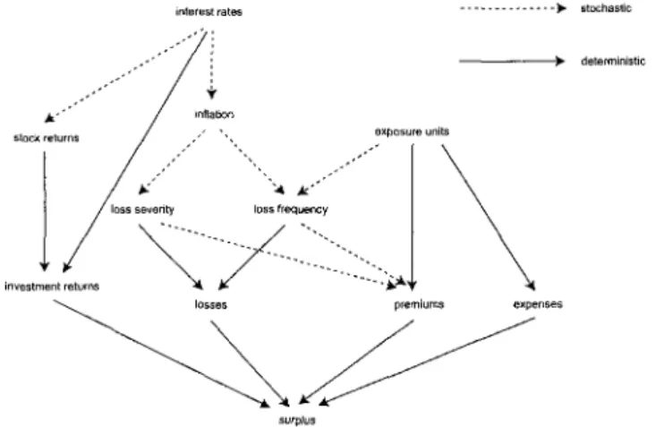
The aim of this section is t o give an example of potential applications of D F A . Figure 4.1 displays the model logic of the approach introduced in this paper in graphical format. By providing a simple example we will show how to analyze surplus a n d ruin probabilities. It was n o t intended t o describe a specific effect when using the parameters given below. T h e parameters were made up, i.e. they were not based on a real case.
Simplifying assumptions • Only one line of business.
• New business and renewal business are not modelled separately. • Payment patterns are assumed t o be deterministic.
• N o transaction costs. • N o taxes.
FIGURE 4.1: Schematic description of the modelling process: stochastic and deterministic influences on surplus.
Model choices
Number of non-catastrophe losses ~ NB (154, 0.025).
Mean severity of non-catastrophe losses ~ Gamma (9.091, 242), inflation-adjusted.
Number of catastrophes ~ Pois (18).
Severity of individual catastrophes ~ lognormal (13, 1.52), inflation-adjusted.
Optional excess of loss reinsurance with deductible 500000 (inflation-adjusted), and cover °o.
Underwriting cycles: 1 = weak, 2 = average, 3 = strong. State in year 0: 1 (weak). Transition probabilities: pu = 60%, pu = 25%, pn = 15%, p2l = 25%, p22 -55%, p23 = 20%, pu = 10%, pn = 25%, p33 = 65%.
All liquidity is reinvested. There are only two investment possibilities: 1) buy a risk-free bond with maturity one year,
2) buy an equity portfolio with a fixed beta.
Market valuation: assets and liabilities are stated at market value, i.e. assets are stated at their current market values, liabilities are discounted at the appropriate term spot rate determined by the model.
Model parameters
• Interest rates, see (2.4): a = 0.25, b = 5%, s = 0.1, rx = 2%. • General inflation, see (2.8): a1 = 0%, b1 = 0.75, a1 = 0.025.
• No inflation impacting the number of claims. • Inflation impacting severity of claims, see (2.10):
ax = 3.5%, bx = 0.5, ax = 0.02.
• Stock returns, see (2.14), (2.15) and (2.16): aM = 4%, bM = 0.5, 0? s 0.5, a - 0.15. • Market share: 5%.
242 R. KAUFMANN, A. GADMER AND R. KLETT
• Expenses: 28.5% of written premiums.
• Premiums for reinsurance: 175 000 p.a. (inflation-adjusted). Historical data
• Written premiums in the last year: 20 million. • Initial surplus: 12 million.
Strategies considered
• Should the company buy reinsurance coverage or not?
• How should the reinvestment of excess liquidity be split between fixed income instruments and stocks?
Projection period
• 10 years (yearly intervals). Risk and return measures
• Return measure: expected surplus E[C/10].
• Risk measure: ruin probability, defined as P[UW < 0].
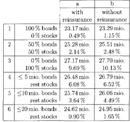
We ran this model 10 000 times for the twelve strategies summarized in Figure 4.2. The first three rows represent a fixed asset allocation. The remaining ones are characterized by an upper limit for the amount of money allowed to be invested in bonds. The amount exceeding this limit is invested in stocks. For each strategy we evaluated the expected surplus and the probability of ruin. Figure 4.3 rules out only one strategy definitely, based on the selected risk and return measures: strategy lb has lower return but higher risk than strategy 6a. If we replace the return measure "expected surplus" by the median surplus, and evaluate the same twelve strategies, we get a completely different picture.
1 2 3 4 5 6 100% bonds 0 % stocks 50% bonds 50 % stocks 0 % bonds 100% stocks < 5 mio. bonds rest stocks < 10 mio. bonds rest stocks <20mio. bonds rest stocks a with reinsurance 23.17 mio. 0.49% 25.28 mio. 2.14% 27.17 mio. 9.69% 26.48 mio. 6.08% 25.74 mio. 3.64% 24.62 mio. 0.90% b without reinsurance 23.29 mio. 1.15% 25.51 mio. 2.48% 27.70 mio. 10.13% 26.79 mio. 6.52% 26.06 mio. 4.49% 24.95 mio. 1.65%
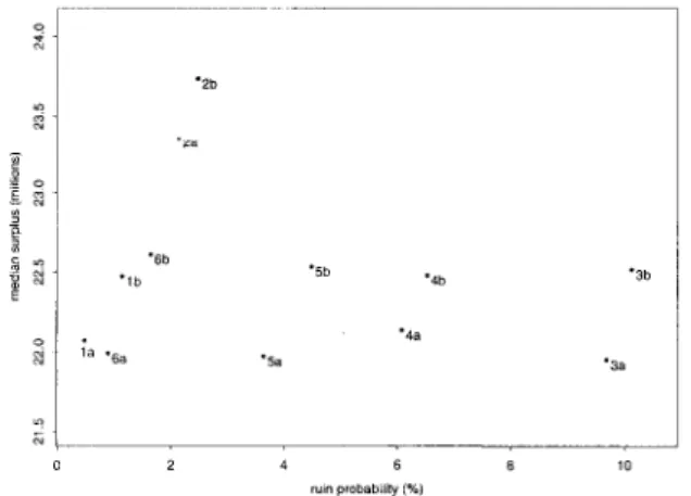
Figure 4.4 shows that by choosing the median surplus as return measure and ruin probability as risk measure all six strategies with a ruin probability above 3% (i.e. strategies 3a, 3b, 4a, 4b, 5a and 5b) are clearly outperformed by the strategies 2a and 2b, where half of the money is invested in bonds and the other half in stocks.
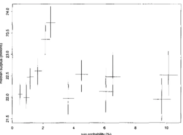
An advantage of median surplus is the fact that one can easily calculate confidence intervals for this return measure. In Figure 4.5 we plotted confi-dence intervals, based on the 10 000 simulations performed. These intervals should be interpreted as 95% confidence intervals for ruin probability given a specific strategy and 95% confidence intervals for median surplus given a spe-cific strategy. Note that Figure 4.5 does not attempt to give joint confidence areas. Furthermore it is important to be aware of the fact that a 95% confi-dence interval for median surplus does not mean that 95% of the simulations at the end of the projection period result in an amount of surplus that lies in this
FIGURR 4.3: Graphical comparison of ruin probabilities and expected surplus for selected business strategies.
ruin probability (%)
FIGURE 4.4: Graphical comparison of ruin probabilities and median surplus for selected business strategies.
244 R. KAUFMANN, A. GADMER AND R. KLETT
FIGURE 4.5: 95% confidence intervals for ruin probability and median surplus, based on 10 000 simulations for each strategy.
interval. The correct interpretation is that given our observed sample of 10 000 simulations, the probability for median surplus lying in this interval is 95%.
5. SOME REMARKS ON DFA
5.1. Discussion Points
This introductory paper discussed only the most relevant issues related to DFA modelling. Therefore, we would like to mention briefly some additional points without necessarily being exhaustive.
5.1.1. Deterministic Scenario Testing
In Section 1 we mentioned the superiority of DFA compared to deterministic scenario testing. This does not imply that the latter method is useless at all. On the contrary, deterministic scenario testing is a very useful thing, in par-ticular when it comes to assess the impact of extreme events at pre-defined dates or when specific macroeconomic influences are to be evaluated. It is a very useful feature of a DFA tool being able to switch off stochasticity and return to deterministic scenarios.
5.1.2. Macroeconomic Environment
In life insurance financial modelling interest rates are often considered to be the only macroeconomic factor affecting the values of assets and liabilities. Hodes, Feldblum and Neghaiwi [21] have pointed out that in nonlife insur-ance, interest rates are only one of various other factors affecting liability val-ues. In Worker's Compensation in the US, for instance, unemployment rates and industrial capacity utilization have greater effects on loss costs than inter-est rates have, while third-party motor claims are correlated with total volume
of traffic and with sales of new cars. Although rarely done it might be worth-while modelling specific macroeconomic drivers like industrial capacity uti-lization or traffic volume separately. This would require a foregoing econo-metric analysis of the dynamics of particular factors.
5.1.3. Correlations
DFA is able to allow for dependencies between different stochastic variables. Before starting to implement these dependencies one should have a sound understanding of existing dependencies within an insurance enterprise. Esti-mating correlations from historical (loss) data is often not feasible due to aggregate figures and structural changes in the past, e.g. varying deductibles, changing policy conditions, acquisitions, spin-offs, etc. Furthermore, recent research, see for example Embrechts, McNeil and Straumann [17] and [18], and Lindskog [28], suggests that linear correlation is not appropriate to model dependencies between heavy-tailed and skewed risks.
We suggest modelling dependencies implicitly, as a result of a number of contributory influences, for example, catastrophes that impact more than one line of business or interest rate changes affecting only specific lines. The majority of these relations should be implemented based on economic and actuarial wisdom, see for instance Kreps [26].
5.1.4. Separate Modelling of New and Renewal Business
In the model outlined in this paper we allowed for separate modelling of new and renewal business, see Section 2.3. Hodes, Feldblum and Neghaiwi [21] pointed out that this makes perfectly sense due to different stochastic beha-viour of the respective loss portfolios. Furthermore, having this split allows a deeper analysis of value drivers within the portfolio and marks an important step towards determining an appraised value for a nonlife insurance company. 5.7.5. Model Validation
What is finally a good DFA model and what is not? Experience, knowledge and intuition of users from actuarial, economic and management side play a dominant role in evaluating a DFA model. A danger in this respect might be that non-intuitive results could be blamed on a bad model instead of wrong assumptions. A further possibility to evaluate a model is to test results com-ing out of the DFA model against empirical results. This will only be feasible in very few restricted cases because it would require keeping track of data for several years. However, model validation should deserve more attention. This needs to be recommended in particular to those practitioners dealing with software vendors of DFA tools who do not intend to justify their decision of buying an expensive DFA product by referring to the software design only.
5.1.6. Model Calibration
We have already touched on this at several places and pointed to its impor-tance within a DFA analysis. However sophisticated a DFA tool or model might be, it has to be fed with data and parameter values. Studies have shown that the major part of a DFA analysis had been devoted to this exercise.